Quantum dynamics in sine-square deformed conformal field theory:
Quench from uniform to non-uniform CFTs

Abstract

In this work, motivated by the sine-square deformation (SSD) for (1+1)-dimensional quantum critical systems, we study the non-equilibrium quantum dynamics of a conformal field theory (CFT) with SSD, which was recently proposed to have continuous energy spectrum and continuous Virasoro algebra. In particular, we study the time evolution of entanglement entropy after a quantum quench from a uniform CFT, which is defined on a finite space of length $L$, to a sine-square deformed CFT. We find there is a crossover time $t^{\ast}$ that divides the entanglement evolution into two interesting regions. For $t\ll t^{\ast}$, the entanglement entropy does not evolve in time; for $t\gg t^{\ast}$, the entanglement entropy grows as $S_{A}(t)\simeq\frac{c}{3}\log t$, which is independent of the lengths of the subsystem and the total system. This $\log t$ growth with no revival indicates that a sine-square deformed CFT effectively has an infinite length, in agreement with previous studies based on the energy spectrum analysis. Furthermore, we study the quench dynamics for a CFT with M$\ddot{\text{o}}$bius deformation, which interpolates between a uniform CFT and a sine-square deformed CFT. The entanglement entropy oscillates in time with period $L_{\text{eff}}=L\cosh(2\theta)$, with $\theta=0$ corresponding to the uniform case and $\theta\to\infty$ corresponding to the SSD limit. Our field theory calculation is confirmed by a numerical study on a (1+1)-d critical fermion chain.

I Introduction

(1+1)-dimensional quantum many-body systems with sine-square deformation (SSD) have been extensively studied in recent years. Gendiar et al. (2009, 2010); Hikihara and Nishino (2011); Gendiar et al. (2011); Shibata and Hotta (2011); Hotta and Shibata (2012); Hotta et al. (2013); Katsura (2011, 2012); Maruyama et al. (2011); Tada (2015); Okunishi and Katsura (2015); Ishibashi and Tada (2015, 2016); Okunishi (2016); Wen et al. (2016); Tamura and Katsura (2017); Tsukasa The SSD was originally introduced as a spatial deformation of Hamiltonian density that efficiently suppresses the boundary effects.Gendiar et al. (2009, 2010); Hikihara and Nishino (2011); Gendiar et al. (2011) The set-up is as follows: Consider a (1+1)-d quantum many-body system with open boundary condition and Hamiltonian

$$H_{0}=\int_{0}^{L}h(x)dx,$$ (1)

where $h(x)$ is the Hamiltonian density. For simplicity, we assume $h(x)$ is uniform. Now we deform the Hamiltonian as follows

$$H_{\text{SSD}}=\int_{0}^{L}2\sin^{2}\left(\frac{\pi x}{L}\right)h(x)dx.$$ (2)

Apparently, the system is disconnected at $x=0$ $(L)$. This kind of deformation shows remarkable properties for (1+1)-d quantum critical systems. It was found that the ground state of (2) is identical to that of a uniform system with periodic boundary condition within numerical accuracy.Hikihara and Nishino (2011); Gendiar et al. (2011); Shibata and Hotta (2011); Hotta and Shibata (2012); Hotta et al. (2013) This property was further verified analytically in some exactly solvable models. Katsura (2011, 2012); Maruyama et al. (2011); Okunishi and Katsura (2015)

Later, the SSD of a two dimensional conformal field theory (CFT) was investigated in Ref.Katsura, 2011, where it is found that the Hamiltonian for a generic CFT with SSD can be expressed as $\mathcal{L}_{0}+\bar{\mathcal{L}}_{0}$, where

$$\mathcal{L}_{0}=L_{0}-\frac{L_{1}+L_{-1}}{2},$$ (3)

and similarly for $\bar{\mathcal{L}}_{0}$. Here $L_{n}$ ($n=0,\pm 1,\cdots$) are Virasoro generators in a CFT. Considering the Hamiltonian (2), since $\sin^{2}(\frac{\pi x}{L})$ vanishes at the boundary, there is no difference in the system between an open boundary condition and a periodic boundary condition. On the other hand, for periodic boundary condition the Hamiltonian (3) has the same ground state as a uniform CFT with Hamiltonian $L_{0}+\bar{L}_{0}$, because in periodic system the CFT vacuum is annihilated by $(L_{1}+L_{-1})/2$ and $(\bar{L}_{1}+\bar{L}_{-1})/2$. With these two observations, the ground state of the SSD system with open boundary condition is the same as that for a uniform system with periodic boundary condition.

In two recent papers by Ishibashi and Tada,Ishibashi and Tada (2015, 2016) they studied the sine-square deformed CFT by dipolar quantization. Choosing different time slices and time translations, they showed that 2d CFTs with SSD have different quantization other than the radial quantization, which is called dipolar quantization. They also found a continuous Virasoro algebra which is labeled by a continuous real index $\kappa$:

$$[\mathcal{L}_{\kappa},\mathcal{L}^{\prime}_{\kappa}]=(\kappa-\kappa^{\prime})\mathcal{L}_{\kappa+\kappa^{\prime}}+\frac{c}{12}\kappa^{3}\delta(\kappa+\kappa^{\prime}),$$ (4)

with $\kappa>0$, and here $c$ is the central charge of the CFT. This continuous Virasoro algebra results in a continuous spectrum in the CFT with SSD, which implies that the sine-square deformed CFT effectively has an infinite length, even though it is defined on a finite space.

To further understand the property of CFTs with SSD, some regularization schemes were proposed recently. Okunishi (2016); Wen et al. (2016) It was found that the connection between the uniform system and the SSD system can be built by considering the parameterized Hamiltonian $\mathcal{L}_{0}+\bar{\mathcal{L}}_{0}$ withOkunishi (2016)

$$\mathcal{L}_{0}=L_{0}-\tanh(2\theta)\frac{L_{1}+L_{-1}}{2},$$ (5)

and similarly for $\bar{\mathcal{L}}_{0}$. Here one can choose $\theta\geq 0$ without loss of generality. It can be checked that the rescaled Hamiltonian $\cosh(2\theta)\cdot\left(\mathcal{L}_{0}+\bar{\mathcal{L}}_{0}\right)$ is related to the conventional one $L_{0}+\bar{L}_{0}$ by a M$\ddot{\text{o}}$bius transformation.Okunishi (2016) For this reason, we will refer to the Hamiltonian defined through Eq.(5) as the M$\ddot{\text{o}}$bius Hamiltonian, and we will call this kind of deformation as M$\ddot{\text{o}}$bius deformation. It is noted that for M$\ddot{\text{o}}$bius deformation, one has a M$\ddot{\text{o}}$bius quantization that bridges the radial quantization for the conventional case and the dipolar quantization for the SSD case. One can refer to Ref.Okunishi, 2016 for more details. Then $\theta=0$ corresponds to the uniform case, and $\theta\to\infty$ corresponds to the SSD limit. Within M$\ddot{\text{o}}$bius deformation, one can find a Virasoro algebra which is the same as Eq.(4), except that now $\kappa$ is not a continuous real index but it has the expression $\kappa=\frac{n}{\cosh(2\theta)},$ where $n$ is an integer. In the SSD limit $\theta\to\infty$, $\kappa$ becomes continuous, which results in a continuous spectrum as observed by Ishibashi and Tada.Ishibashi and Tada (2015, 2016)

I.1 Our motivation

Based on the introduction above, now let us state our motivations in this work:

1. Given the continuous energy spectrum for a CFT with SSD, how does it affect the non-equilibrium quantum dynamics? To avoid any operator dependence, we will study the entanglement evolution in quench dynamics. It is interesting to see if there is any universal feature in the entanglement evolution, and if yes, how it is related with the continuous spectrum. As far as we know, there is no work studying the entanglement property of a CFT with SSD in the non-equilibrium case.

2. Since the M$\ddot{\text{o}}$bius Hamiltonian [see Eq.(5)] interpolates between the uniform system and SSD system. It is also interesting to study the quench dynamics governed by this Hamiltonian, and see how it behaves as we approach the SSD limit.

3. There is much recent interest in studying the entanglement property in CFT in curved spacetime (See, e.g., Refs.Refael and Moore, 2004; Rodríguez-Laguna et al., 2016; Dubail et al., 2017a; Viti et al., 2016; Eisler and Bauernfeind, 2017; Dubail et al., 2017b; Tonni et al., ; Ramírez et al., 2015; Rodríguez-Laguna et al., 2017.) One interesting setup is based on the inhomogeneous Hamiltonian density.Dubail et al. (2017b) We hope that our work will provide a nice setup and approach in this direction.

The rest of this paper is organized as follows: In Sec.II, we introduce our setup of quantum quench, and study the entanglement evolution after a quantum quench from a uniform system to a SSD system. Then in Sec.III, we study the quench dynamics for the M$\ddot{\text{o}}$bius case, and see how it connects the uniform and SSD cases. In Sec.IV, we present some discussions and conclude our work. In Appendix A, we introduce the lattice model based on which we do numerical calculations. In Appendix B, we interpret the SSD and M$\ddot{\text{o}}$bius Hamiltonian as a CFT in curved spacetime.

Figure 1: For $t<0$, we prepare our initial state as the ground state of a uniform CFT with open boundary condition. From $t=0$, we evolve the initial state with a sine-square deformed Hamiltonian. The red solid lines represent the strength of Hamiltonian density. The lattice represents a microscopic model that may realize the CFT in IR limit.

II Entanglement evolution:
Quench from uniform to SSD systems

II.1 Setup

There are several interesting setups for quantum quenches, such as the global quench,Calabrese and Cardy (2005, 2007a, 2016) local quench,Calabrese and Cardy (2007b); Nozaki et al. (2014); He et al. (2014); Stéphan and Dubail (2011) and inhomogeneous quantum quench. Sotiriadis and Cardy (2008); Viti et al. (2016); Dubail et al. (2017a); Eisler and Bauernfeind (2017); Bertini et al. (2016); Dubail et al. (2017b); Bertini et al. (2018); Wen et al. (2018); Brun and Dubail (2017)

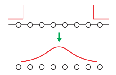
Here, we consider a quantum quench from a uniform CFT to a non-uniform CFT. As shown in Fig.1, we prepare our initial state as the ground state $|G\rangle$ of a uniform CFT on a finite space $[0,L]$, with an open boundary condition. (The reason we do not choose a periodic boundary condition (PBC) is that, as mentioned in the introduction, a critical system with a PBC shares the same ground state with the SSD system, and no quench is expected to happen in this case. It is noted, however, that there may be some difference in the ground states at UV scale. We are not interested in quantum quench in this case, the feature of which is non-universal.) Then at $t=0$, we switch the Hamiltonian to the sine-square deformed one. Then the time dependent state can be written as $|\psi(t)\rangle=e^{-iH_{\text{SSD}}t}|G\rangle$. The correlation function of $O(x_{1})\cdots O(x_{n})$ at time $t$ can be expressed as $\langle G|e^{iH_{\text{SSD}}t}O(x_{1})\cdots O(x_{n})e^{-iH_{\text{SSD}}t}|G\rangle$.

Throughout this work, to study the quench dynamics of a sine-square deformed CFT, we are interested in the time evolution of entanglement entropy for a subsystem $A=[0,l]$. The entanglement measure we use is the so-called Renyi entropy

$$S_{A}^{(n)}(t)=\frac{1}{1-n}\log\text{tr}\left[\rho_{A}^{n}(t)\right],$$ (6)

and the von-Neumann entropy

$$S_{A}(t)=\lim_{n\to 1}S_{A}^{(n)}(t).$$ (7)

The term $\text{tr}(\rho_{A}^{n})$ in $S_{A}^{(n)}(t)$ is related with the single-point correlation function of twist operator as follows:Calabrese and Cardy (2009)

$$\text{tr}(\rho_{A}^{n})=\langle G|e^{iH_{\text{SSD}}t}\mathcal{T}_{n}(x=l)e^{-iH_{\text{SSD}}t}|G\rangle,$$ (8)

where $\mathcal{T}_{n}$ is a primary operator with conformal dimension

$$h=\frac{c}{24}\left(n-\frac{1}{n}\right),$$ (9)

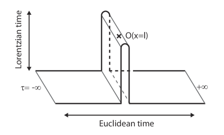
In the following, we will evaluate the correlation function in Eq.(8) with path integral method. Pictorially, $\langle\psi(t)|\mathcal{T}_{n}(x=l)|\psi(t)\rangle$ is shown in Fig.2 by setting $O(x)=\mathcal{T}_{n}(x)$. Note that there are both Euclidean time and Lorentzian time in the path integral. As shown in the following part, we will do calculation in the Euclidean spacetime by setting $it=\tau$, and analytically continue back to Lorentzian time in the final step.

Figure 2: Path integral representation for the correlation function $\langle G|e^{iH_{\text{SSD}}t}\mathcal{O}(x=l)e^{-iH_{\text{SSD}}t}|G\rangle$. The ground state $|G\rangle$ of Hamiltonian $H_{0}$ can be considered as the path integral starting from $\tau=-\infty$ and evolving to $\tau=0$ according to Hamiltonian $H_{0}$. The width of this strip is $L$. Then the ground state evolves in the Lorentzian time direction according to the new Hamiltonian $H_{\text{SSD}}$. After inserting an operator $\mathcal{O}(x)$ at $x=l$, we evolve the state back to $\tau=0$. Then the state evolves to $\tau=+\infty$ with $H_{0}$.

II.2 Entanglement evolution after a quantum quench from uniform to SSD systems

To study the entanglement entropy evolution, we will go to Euclidean spacetime by setting $it=\tau$. Then the correlation function in Eq.(8) has the form

$$\langle G\mid e^{H_{\text{SSD}}\tau}\mathcal{T}_{n}^{(w)}(w_{0},\bar{w}_{0})e^{-H_{\text{SSD}}\tau}\mid G\rangle.$$ (10)

Here in the Euclidean plane $w=\tau+i\sigma$, one has $-\infty<\tau<\infty$, $0\leq\sigma\leq L$, and $w_{0}=0+il$ ($0\leq l\leq L$) is used to label the position of the twist operator. The superscript $(w)$ in $\mathcal{T}^{(w)}_{n}$ denotes the coordinate. Two conformal boundary conditions are imposed along $\sigma=0$ and $L$, respectively. For simplicity, we assume the two boundary conditions are the same.

To evaluate the correlation function in Eq.(10), we take the following two strategies:

(i) Heisenberg picture. Instead of evolving the states, we will evolve the operator $\mathcal{T}_{n}$ with the Hamiltonian $H_{\text{SSD}}$ in Heisenberg picture. By conformal transformation into a certain coordinate, it is quite straightforward to write down the operator’s evolution.

(ii) We start from M$\ddot{\text{o}}$bius Hamiltonian $H_{\text{ M$\ddot{\text{o}}$b}}(\theta)$ first. Taking $\theta\to\infty$, we can read out the SSD result. As we mentioned in the introduction, the SSD Hamiltonian has a continuous spectrum. In case of unnecessary IR problem, we regard the M$\ddot{\text{o}}$buis Hamiltonian as a regularization of SSD. To be concrete, in terms of stress-energy tensor $T$, the Hamiltonian $H_{\text{ M$\ddot{\text{o}}$b}}(\theta)$ in $w$-plane can be written asOkunishi (2016)

$$H_{\text{M$\ddot{\text{o}}$b}}=H_{0}-\frac{\tanh(2\theta)}{2}\left(H_{+}+H_{-}\right),$$ (11)

where

$$H_{0}=\int_{0}^{L}\frac{d\sigma}{2\pi}T_{\tau\tau}(\sigma)=\int_{0}^{L}\frac{d\sigma}{2\pi}(T(w)+\bar{T}(\bar{w})),$$ (12)

and

$$H_{\pm}=\int_{0}^{L}\frac{d\sigma}{2\pi}\left(e^{\pm 2\pi w/L}T(w)+e^{\mp 2\pi\bar{w}/L}\bar{T}(\bar{w})\right).$$ (13)

Apparently, for $\theta\to\infty$ we have $H_{\text{M$\ddot{\text{o}}$bius}}(\theta\to\infty)=H_{0}-\frac{1}{2}(H_{+}+H_{-})$, which is the SSD Hamiltonian.Katsura (2011)

Based on the above two strategies, we are ready to calculate the correlation function in Eq.(10). Readers who are not interested in the technical part can go to the result in Eq.(27) directly. Now let us consider the conformal mapping

$$z=e^{\frac{2\pi}{L}w},$$ (14)

which maps the strip in $w$-plane to a complex $z$-plane. The two boundaries along $\sigma=0,\,L$ in $w$-plane are mapped to a slit along $z=x\pm i0$, with $x\in[0,\infty)$. The holomorphic part of $H_{\text{M$\ddot{\text{o}}$b}}$ in $z$-plane is

$$\begin{split}H_{\text{M$\ddot{\text{o}}$b}}^{(z)}=&\frac{2\pi}{L\cosh(2\theta)}\Big{[}\cosh(2\theta)\oint\frac{zdz}{2\pi i}zT(z)\\ &-\frac{\sinh(2\theta)}{2}\oint\frac{z^{2}+1}{2\pi i}T(z)dz\Big{]}-\frac{\pi c}{12L}.\end{split}$$ (15)

Apparently, the Hamiltonian $H_{\text{M$\ddot{\text{o}}$b}}^{(z)}$ is still complicate and we do not know how to act it on the primary field. It is found that one can use a M$\ddot{\text{o}}$bius transformation to further map it to $\tilde{z}$-plane: Okunishi (2016)

$$\tilde{z}=f(z)=-\frac{\cosh\theta z-\sinh\theta}{\sinh\theta z-\cosh\theta}.$$ (16)

Then the holomorphic part of $H_{\text{M$\ddot{\text{o}}$b}}$ has the simple form

$$\begin{split}H_{\text{M$\ddot{\text{o}}$b}}^{(\tilde{z})}=&\frac{1}{iL\cosh(2\theta)}\oint\tilde{z}T(\tilde{z})d\tilde{z}-\frac{\pi c}{12L}\\ =&\frac{2\pi}{L\cosh(2\theta)}L_{0}^{(\tilde{z})}-\frac{\pi c}{12L}.\end{split}$$ (17)

It is similar for the anti-holomorphic part of $H_{\text{M$\ddot{\text{o}}$b}}^{(\tilde{z})}$. Then we have

$$e^{H_{\text{M$\ddot{\text{o}}$b}}\tau}\mathcal{T}_{n}^{(\tilde{z})}(\tilde{z},\bar{\tilde{z}})e^{-H_{\text{M$\ddot{\text{o}}$b}}\tau}=\lambda^{2h}\mathcal{T}_{n}^{(\tilde{z})}(\lambda\tilde{z},\lambda\bar{\tilde{z}}),$$ (18)

which is nothing but the dilatation operation in $\tilde{z}$-plane. Here $h$ is the conformal dimension of $\mathcal{T}_{n}$ in Eq.(9), and

$$\lambda:=\exp\left(\frac{2\pi\tau}{L\cosh(2\theta)}\right).$$ (19)

Back in $z$-plane, its effect is to shift the operator $\mathcal{T}_{n}^{(z)}$ from $z$ to $z_{\text{new}}$, where $z_{\text{new}}$ is related with $z$ as

$$f(z_{\text{new}})=\lambda f(z),$$ (20)

with $f(z)$ given in Eq.(16). Then one can obtain

$$z_{\text{new}}=\frac{[(1-\lambda)\cosh 2\theta-(\lambda+1)]z+(\lambda-1)\sinh 2\theta}{(1-\lambda)\sinh 2\theta\cdot z+[(\lambda-1)\cosh 2\theta-(\lambda+1)]}.$$ (21)

Therefore, the correlation function of $\mathcal{T}_{n}$ can be written as:

$$\begin{split}&\langle G\mid e^{H_{\text{M$\ddot{\text{o}}$b}}\tau}\mathcal{T}_{n}^{(w)}(w_{0},\bar{w}_{0})e^{-H_{\text{M$\ddot{\text{o}}$b}}\tau}\mid G\rangle\\ =&\left(\frac{\partial z}{\partial w}\right)^{h}\left(\frac{\partial\bar{z}}{\partial\bar{w}}\right)^{h}\left(\frac{\partial z_{\text{new}}}{\partial z}\right)^{h}\left(\frac{\partial\bar{z}_{\text{new}}}{\partial\bar{z}}\right)^{h}\left\langle\mathcal{T}_{n}^{(z)}(z_{\text{new}},\bar{z}_{\text{new}})\right\rangle.\end{split}$$ (22)

Here $\langle\mathcal{T}^{(z)}_{n}(z,\bar{z})\rangle$ is the one point correlation function in a boundary CFT. The boundary condition is imposed along the slit $z=x\pm i0$ on real axis, with $x\in[0,\infty)$. Explicitly, $\langle\mathcal{T}^{(z)}_{n}(z,\bar{z})\rangle$ can be expressed as

$$\langle\mathcal{T}^{(z)}_{n}(z,\bar{z})\rangle=A_{n}^{\text{b}}\cdot(\frac{1}{4}z^{-\frac{1}{2}}\bar{z}^{-\frac{1}{2}})^{h}\cdot(\frac{2ai}{z^{\frac{1}{2}}-\bar{z}^{\frac{1}{2}}})^{2h},$$ (23)

where $A^{\text{b}}_{n}$ is an amplitude depending on the selected boundary condition, which will affect the entanglement entropy by an order $\sim\mathcal{O}(1)$ term. $a$ is a UV cut-off, which may be considered as the lattice spacing in a microscopic lattice model.

Recall that in the procedures above, the Hamiltonian we use is $H_{\text{M$\ddot{\text{o}}$b}}(\theta)$. One needs to further take $\theta\to\infty$ to obtain the SSD limit. After some tedious but straightforward steps, finally we arrive at

$$\begin{split}&\langle G\mid e^{H_{\text{SSD}}\tau}\mathcal{T}_{n}^{(w)}(w_{0},\bar{w}_{0})e^{-H_{\text{SSD}}\tau}\mid G\rangle\\ =&A^{\text{b}}_{n}\left(\frac{2\pi^{2}a^{2}}{L^{2}}\right)^{h}\cdot\left(\frac{1}{m(t)^{2}+m(t)\cdot n(t)}\right)^{h},\end{split}$$ (24)

where

$$m(t)=\sqrt{n(t)^{2}+\sin^{2}\frac{2\pi l}{L}},$$ (25)

and

$$n(t)=\left(1-\cos\frac{2\pi l}{L}\right)\frac{2\pi^{2}t^{2}}{L^{2}}-\cos\frac{2\pi l}{L}.$$ (26)

Here we have already taken the analytical continuation $\tau\to it$. Then based on Eqs.(6)$\sim$(8), one can obtain the entanglement entropy for $A=[0,l]$ as follows

$$S_{A}(t)=\frac{c}{12}\log\left\{\frac{L^{2}}{2\pi^{2}a^{2}}\cdot\left[m(t)^{2}+m(t)\cdot n(t)\right]\right\},$$ (27)

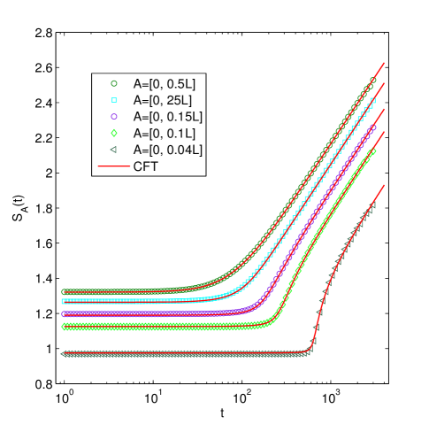
where we have neglected the $\mathcal{O}(1)$ term $\sim c\log A_{n=1}^{b}$ contributed by the conformal boundary condition. As shown in Fig.3, we compare our field theory result $S_{A}(t)$ with the numerical calculation on a lattice fermion chain (See the appendix for numerics. The only fitting parameter we used is the global constant shift in the ground-state entanglement entropy $S_{A}(t=0)$. It is noted that for a free fermion model, this constant term in $S_{A}(t=0)$ has been exactly evaluated in Ref.Fagotti and Calabrese, 2011.). They agree in an excellent way. One remarkable feature is that the entanglement entropy $S_{A}(t)$ grows as $S_{A}(t)\simeq\frac{c}{3}\log t$ in the long time limit. Although the system is defined on a finite space $[0,L]$, in contrast to the uniform CFT,Cardy (2014) no revival appears here. This agrees with previous observations that a CFT with SSD effectively has an infinite length limit. In our case, the signal caused by a quench can never reach the ‘boundary’ of the SSD system and reflect back. One intuitive picture is to consider the sine-square deformation directly. Since $\sin^{2}\frac{\pi x}{L}$ vanishes near the boundaries $x=0,\,L$, the local group velocity of quasi-particles $v(x)=2\sin^{2}\frac{\pi x}{L}$ will go to zero when approaching the boundary. Then it takes an infinite time for the quasiparticles to reach the boundary and reflect back. We will give further discussion on this effect in next section.

It is noted that there is much more information in $S_{A}(t)$ in Eq.(27) and Fig.3, which we will analyze case by case in the following:

Figure 3: Comparison between numerical results and CFT calculation for entanglement entropy evolution $S_{A}(t)$ after a quantum quench from a uniform CFT to a sine-square deformed CFT. Here we choose $L=500$.

(i) $t=0$

This corresponds to the ground state of a CFT with open boundary condition. $S_{A}(t)$ in Eq.(27) can be simplified as

$$S_{A}(t=0)=\frac{c}{6}\log\left[\frac{L}{\pi a}\sin\left(\frac{\pi l}{L}\right)\right].$$ (28)

This is the well known result for a finite interval of length $l$ at the end of a CFT living on $[0,L]$.Calabrese and Cardy (2004)

(ii) $l=L/2$, $t>0$

Now the subsystem is the left half (or right half) of the total system. $S_{A}(t)$ has a very simple expression as follows

$$S_{A}(t)=\frac{c}{6}\log\left[\frac{1}{a^{2}}\Big{(}t^{2}+\frac{L^{2}}{4\pi^{2}}\Big{)}\right]-\frac{c}{6}\log\left(\frac{L}{4\pi a}\right).$$ (29)

One can find there is a crossover around $t^{\ast}=L/2\pi$ (see also Fig.3). For $t\ll t^{\ast}$, $S_{A}(t)=\frac{c}{6}\log(L/\pi a)$ is independent of time; while for $t\gg t^{\ast}$, $S_{A}(t)\simeq\frac{c}{3}\log t$, which is universal and independent of $l$ and $L$, as can be observed in Fig.3.

(iii) $l\ll L$, $t>0$

As shown in in Fig.3, for arbitrary $l\in(0,L)$, there is a crossover time $t^{\ast}$, so that for $t\ll t^{\ast}$ one has $S_{A}(t)\simeq S_{A}(t=0)$, and for $t\gg t^{\ast}$ one has $S_{A}(t)\simeq\frac{c}{3}\log t$. In particular, for $l\ll L$, one can find a simple expression of $t^{\ast}$ as follows:

$$\boxed{t^{\ast}=\frac{L^{2}}{2\pi^{2}l}}\,,\quad l\ll L.$$ (30)

When the length $L$ of total system is fixed, one can find that $t^{\ast}\propto l^{-1}$. This explains why there is a wider plateau for smaller $l$ in Fig.3. In other words, the smaller $l$ is, the longer time $S_{A}(t)$ stays in its initial value $S_{A}(t=0)$. This may be intuitively understood as follows. Since the Hamiltonian density is sine-square deformed, the local group velocity of quasi-particles also varies in position. The group velocity is smaller near the boundary, and larger near the center of the system. If the entanglement cut is close to the boundary (this corresponds to $l\ll L$ or $L-l\ll L$), it takes the quasi-particles longer time to reach (or escape) subsystem $A$. Therefore, $S_{A}(t)$ will stay at its initial value for a longer time.

For general $l\in(0,L)$, the crossover time $t^{\ast}$ is determined by

$$t^{\ast}=\frac{L}{2\pi}\cdot\sin^{-1}\Big{(}\frac{\pi l}{L}\Big{)}\cdot\sqrt{\text{max}\left(\Big{|}\cos\frac{2\pi l}{L}\Big{|},\,\Big{|}\sin\frac{2\pi l}{L}\Big{|}\right)}.$$ (31)

We emphasize that for $t\gg t^{\ast}$, the entanglement entropy grows as $S_{A}(t)\simeq\frac{c}{3}\log t$ all the way, with no revival. This is the feature of an infinite system. On the other hand, in the works by Ishibashi and Tada,Ishibashi and Tada (2015, 2016), it was found that the energy spectrum of a CFT with SSD is continuous. Recall that a uniform CFT on a finite space of length $L$ has energy spacing $\sim 1/L$, which is discrete for a finite $L$. From this point of view, a CFT with SSD seems to have an infinite length limit. Here, we studied this effect from the time evolution of entanglement entropy after a quantum quench.

As a remark, it is noted that in the CFT calculation the entanglement entropy grows as $S_{A}(t)\simeq\frac{c}{3}\log t$ with no upper bound in the long time limit. Apparently, this is not the case for a lattice model, since there is a finite number of degrees of freedom in a subsystem of finite length and the energy spectrum is of finite width. In a lattice model, the entanglement entropy will finally saturate. One can refer to Ref.Wen and Wu, 2018 for more related discussions.

II.3 Physical interpretation of $t^{\ast}$

To further understand the physical meaning of $t^{\ast}$ in Eq.(30), again, it is helpful to consider the quasi-particle picture. Compared to the cases of global quench,Calabrese and Cardy (2005, 2007a, 2016) local quench,Calabrese and Cardy (2007b); Nozaki et al. (2014); He et al. (2014); Stéphan and Dubail (2011) and inhomogeneous quantum quench, Sotiriadis and Cardy (2008); Viti et al. (2016); Dubail et al. (2017a); Eisler and Bauernfeind (2017); Bertini et al. (2016); Dubail et al. (2017b); Bertini et al. (2018); Wen et al. (2018) there is a fundamental difference here. In our case, since the initial state is the ground state of a uniform CFT, which is long-range entangled, there is not an intuitive picture on how the entangled pairs of quasi-particles are distributed in the initial state.

To discuss the physical meaning of $t^{\ast}$, we assume that the quasi-particles are emitted from the main bulk of the system, and then we check the time scale that these quasi-particles propagate into the region $(0,l)$ with $l\ll L$. This assumption is quite reasonable because the Hamiltonian density $2\sin^{2}\left(\frac{\pi x}{L}\right)h(x)$ is more uniform near the two ends of the SSD system, and looks almost the same as the uniform Hamiltonian density $h(x)$ up to a global factor. Then in the quantum quench by evolving the ground state of $H_{0}$ with $H_{\text{SSD}}$, the quasi-particles are mainly emitted from the bulk of the system.

Now we consider the quasiparticles emitted from $\xi$, with $\xi\sim\mathcal{O}(L)$. These quasi-particles will contribute to the entanglement entropy of $A=(0,l)$ after a time

$$t_{q}=\int_{l}^{\xi}\frac{dx}{v(x)}.$$ (32)

Here $v(x)=2\sin^{2}\left(\frac{\pi x}{L}\right)$ is the group velocity of quasi-particles at $x$. It is straightforward to obtain

$$t_{q}=\frac{L}{2\pi}\left(\frac{1}{\tan\frac{\pi l}{L}}-\frac{1}{\tan\frac{\pi\xi}{L}}\right).$$ (33)

Recall that $l\ll\xi$ and $l\ll L$, then $t_{q}$ can be further simplified as

$$t_{q}\simeq\frac{L^{2}}{2\pi^{2}l},$$ (34)

which is nothing but $t^{\ast}$ in Eq.(30). That is, $t^{\ast}$ actually characterizes the light-cone of quasiparticles that enter the subsystem $A=(0,l)$. This explains why for $t\ll t^{\ast}$, the entanglement entropy $S_{A}(t)$ of $A=(0,l)$ does not increase, while for $t\sim t^{\ast}$, the entanglement entropy starts to grow in time.

For a generic $l$ which is of order $\mathcal{O}(L)$, to have a quasi-particle interpretation of $t^{\ast}$ in Eq.(31), one needs to know more concrete information about the distribution of entangled pairs of quasi-particles in the initial state, which is beyond the scope of our current work.

III Entanglement evolution:
Quench from uniform to M$\ddot{\text{o}}$bius deformed systems

Figure 4: Comparison between numerical results and CFT calculation for entanglement entropy evolution after a quantum quench from a uniform CFT to a M$\ddot{o}$bius deformed CFT. It is found that the period of oscillations is $L\cosh(2\theta)$ and the amplitude of oscillation is $2\theta/3$. Here we choose $l=L/2$ with $L=500$.

In the previous section, we have studied the quantum quench from a uniform system to a SSD system. It is natural to ask the following: what happens for the M$\ddot{\text{o}}$bius deformation? It is interesting to see how the M$\ddot{\text{o}}$bius deformation interpolates between the uniform and SSD cases.

To be concrete, we prepare the initial state as the ground state of a uniform CFT on a finite space $[0,L]$. Starting from $t=0$, we have the initial state evolve according to the M$\ddot{\text{o}}$bius Hamiltonian in Eq.(11), and we study the time evolution of entanglement entropy. The procedures are almost the same as those in Sec.II, except that now we do not take the limit $\theta\to\infty$. After some straightforward algebra, one can find the time evolution of entanglement entropy for subsystem $A=[0,l]$ as

$$S_{A}(t)=\frac{c}{12}\log\left\{\frac{L^{2}}{2\pi^{2}a^{2}}\left[f(t)^{2}+f(t)\cdot h(t)\right]\right\},$$ (35)

where, as before, we have neglected the $\mathcal{O}(1)$ contribution from the conformal boundary condition. $f(t)$ and $h(t)$ have the expressions:

$$f(t)=\sqrt{h(t)^{2}+\sin^{2}\frac{2\pi l}{L}},$$ (36)

and

$$\begin{split}h(t)=&-\left(\sin^{2}\frac{\pi t}{L_{\text{eff}}}\cdot\cosh(4\theta)+\cos^{2}\frac{\pi t}{L_{\text{eff}}}\right)\cdot\cos\frac{2\pi l}{L}\\ &+\sin^{2}\frac{\pi t}{L_{\text{eff}}}\cdot\sinh(4\theta),\end{split}$$ (37)

where

$$L_{\text{eff}}=L\cosh(2\theta).$$ (38)

This effective length can be alternatively obtained by considering a CFT in curved spacetime (see Appendix B). As a self-consistent check, one can find that $S_{A}(t)$ reduces to Eq.(28) for $t=0$, and reduces to Eq.(27) for $\theta\to\infty$, as expected.

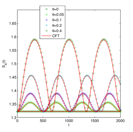
The comparison between CFT results and the numerical calculation is shown in Fig.4, and the agreement is excellent. For $\theta=0$, since the M$\ddot{\text{o}}$bius Hamiltonian is the same as the uniform case, then there is essentially no quench (see Fig.4). For $\theta>0$, it is interesting that oscillations appear in $S_{A}(t)$. Based on $S_{A}(t)$ in Eqs.(35)$\sim$(38), one can find the period of oscillations is $L_{\text{eff}}=L\cosh(2\theta)$. For $\theta\to 0$, the oscillation period is $L$, which is as expected for a uniform CFT. On the other hand, in the SSD limit $\theta\to\infty$, the oscillation period becomes $L\cosh(2\theta)\to\infty$. This agrees with the fact that there is no revival in $S_{A}(t)$ for a CFT with SSD.

To see the features of $S_{A}(t)$ in Eq.(35) more clearly, let us focus on the case $l=L/2$. Then $S_{A}(t)$ can be simplified as

$$S_{A}(t)=\frac{c}{6}\log\left\{\frac{L}{\pi a}\left[\sin^{2}\left(\frac{\pi t}{L_{\text{eff}}}\right)e^{4\theta}+\cos^{2}\left(\frac{\pi t}{L_{\text{eff}}}\right)\right]\right\}.$$ (39)

The period of oscillations with $T=L_{\text{eff}}=L\cosh(2\theta)$ can be explicitly seen in this expression. In addition, one can find that the amplitude of oscillations grows as we increase $\theta$. For $l=L/2$, the amplitude of oscillations has a very simple expression

$$S_{A}(t=\frac{L_{\text{eff}}}{2})-S_{A}(t=0)=\frac{2c}{3}\theta,$$ (40)

which grows with $\theta$ linearly, as can be observed in Fig.4.

Furthermore, it is straightforward to check that as $\theta\to\infty$, the entanglement entropy evolution in Eq.(35) will reduce to the SSD case in Eq.(27), as expected.

As a short summary, by studying the quench dynamics in a CFT with M$\ddot{\text{o}}$bius deformation, one can find that the effective length of the system becomes $L_{\text{eff}}=L\cosh(2\theta)$, which interpolates between the uniform and SSD systems, as we tune $\theta$ from $0$ to $\infty$.

Remark: It is noted that the effective length $L_{\text{eff}}$ can also be understood based on the quasiparticle picture. For the M$\ddot{\text{o}}$bius deformation, the group velocity of quasi-particles at $x$ is $v(x)=1-\tanh(2\theta)\cos\frac{2\pi x}{L}$. Since the system is symmetric about $x=L/2$, for an entangled pair of quasiparticles emitted from $x$, they will meet again at $L-x$ at time

$$t_{q}=\int_{0}^{L}\frac{dx}{v(x)}=L\cosh(2\theta).$$ (41)

Similarly, the entangled-pair of quasiparticles emitted from $L-x$ will meet again for the first time at $x$ with time $t_{q}=L\cosh(2\theta)$. This explains why we observe a revival of $S_{A}(t)$ with a time period $L\cosh(2\theta)$.

IV Concluding remarks

Let us first summarize our main results, and then make some comments.

We studied analytically the quench dynamics of a sine-square deformed CFT, which was proposed to have continuous energy spectrum and infinite length limit. By quenching from a uniform CFT to a sine-square deformed CFT on $[0,L]$, it was found that the entanglement entropy $S_{A}(t)$ for subsystem $A=[0,l]$ evolves in time in a universal way. There exists a crossover time $t^{\ast}$. For $t\ll t^{\ast}$, $S_{A}(t)$ does not evolve in time; for $t\gg t^{\ast}$, $S_{A}(t)$ grows in time all the way as $S_{A}(t)\simeq\frac{c}{3}\log t$, with no revival. This feature indicates that the CFT with SSD effectively has an infinite length limit, consistent with previous analysis on the energy spectrum. In addition, we studied analytically the quench dynamics of a M$\ddot{\text{o}}$bius deformed CFT. Aside from some interesting features, it was found that a length scale $L_{\text{eff}}=L\cosh(2\theta)$ appears in the time evolution of the entanglement entropy, which interpolates between the uniform and SSD systems. We hope our work can stimulate more interest in the non-equilibrium dynamics in sine-square deformed CFTs and other related non-uniform CFTs.

As will be studied in Ref.Wen and Wu, 2018, the setup in this work provides a building block for studying the Floquet dynamics in a conformal field theory. That is, one can drive a CFT with Hamiltonians $H_{0}$ and $H_{\text{SSD}}$ [see Eqs.(1) and (2)] periodically, and see if the system can be heated or not. Compared to the previous work on boundary-driven CFT, Berdanier et al. (2017) now we have a bulk-driven Floquet CFT which can be analytically solved.Wen and Wu (2018)

In addition, careful readers may have noticed that when evaluating the correlation function in Eq.(10), we did not introduce any UV regularization, in contrast to other setups such as Refs.Calabrese and Cardy, 2005, 2007a, 2016, 2007b; Nozaki et al., 2014; He et al., 2014; Stéphan and Dubail, 2011. The reason is as follows. The effect of time evolution operator $U(t)=e^{-iH_{\text{SSD}}t}$ is simply to evolve the primary operator $\mathcal{O}(z,\bar{z})$ to $\mathcal{O}(z_{\text{new}},\bar{z}_{\text{new}})$. The rest of the calculation is essentially evaluating the correlation function within the ground state of $H_{0}$. This is in contrast to other setups where the evaluation of correlation functions cannot be reduced to the calculation within the ground state of $H_{0}$.

There are many open questions and we would like to mention some of them here:

– In our work, we quench a uniform CFT to a non-uniform CFT. There are many other interesting setups for quantum quenches, which may be used to study the property of sine-square deformed CFTs, such as the global and local quenches as introduced in Refs.Calabrese and Cardy, 2007a, b. Technically, it will be more involved to study these setups because the CFT with SSD is defined on a finite space. There are more boundaries introduced by the global/local quenches, and one needs complicate conformal mappings to study these quenches. We also want to point out that there are other interesting entanglement measures that may be helpful to detect how the entanglement is generated (or propagates) in a CFT with SSD. See, e.g., Fig.10 in Ref.Wen et al., 2015, on how to use entanglement negativity to detect the distribution of EPR pairs in a CFT after a quantum quench.

– It is also interesting to study other kinds of deformations, such as a $\sin^{n}$ deformation. It is expected that the Virasoro generators $L_{n}$ and $L_{-n}$ with $n>1$ will also appear in the Hamiltonian. The feature of energy spectrum for CFTs with such deformations was even not well understood. It is interesting to see if such deformations can be analytically studied within the CFT approach.

– Recently, measuring the time evolution of (Renyi) entanglement entropy after a quantum quench was realized in cold atom experiments,Kaufman et al. (2016) where the (1+1)-d quantum system is quenched from a Mott insulator phase to a superfluid phase. Here, the setup in our work applies to arbitrary (1+1)-d quantum critical systems that can be described by a CFT. We expect that our setup may be realized in cold-atom experiments by tuning the tunneling strength between neighboring sites through the optical lattice depth. Bakr et al. (2009) It is noted that the tunneling strength corresponds to the hopping strength in the lattice model (see Appendix A). By tuning the tunneling strength in space in a sine-square deformed way, one may realize SSD as well as its quech dynamics in experiments.

V Acknowledgement

We thank Shinsei Ryu for helpful discussions on various properties of SSD, and thank Chenjie Wang for discussions on CFT in curved spacetime which stimulates our interest in studying this problem, and introducing their recent work [Bao et al., ] to us. We also thank Erik Tonni for discussions on entanglement entropy of 2d CFT in curved spacetime, and thank Wenchao Xu for discussions on the possible realization of our setup in cold atom experiments. XW is supported by the Gordon and Betty Moore Foundation’s EPiQS initiative through Grant No. GBMF4303 at MIT. JQW is supported by Massachusetts Institute of Technology and the Simons foundation it from qubit collaboration.

Appendix A Lattice model

To confirm our field theory result in the main text, we calculate the entanglement entropy evolution based on a free fermion lattice model. We prepare the initial state as the ground state $|G\rangle$ of a uniform free fermion chain with half-filling:

$$H_{0}=\sum_{i=1}^{L-1}hc_{i}^{{\dagger}}c_{i+1}+h.c.,$$ (42)

where $h$ is the hopping strength, and we choose $h=1/2$ throughout the calculation. The length of the chain is $L$ and open boundary condition is imposed. $c_{i}$ ($c_{i}^{{\dagger}}$) are fermionic operators, which satisfy the anticommutation relations $\{c_{i},c_{j}\}=\{c_{i}^{{\dagger}},c_{j}^{{\dagger}}\}=0$, and $\{c_{i},c_{j}^{{\dagger}}\}=\delta_{ij}$.

Then at time $t=0$, we have the initial state $|G\rangle$ evolve according to the new hamiltonian, which is non-uniform in space:

$$H_{1}=\sum_{i=1}^{L-1}\left[1-\tanh(2\theta)\cdot\cos\left(\frac{2\pi(i+1/2)}{L}\right)\right]c_{i}^{{\dagger}}c_{i+1}+h.c.$$ (43)

Note that for $\theta=0$, $H_{1}$ corresponds to the uniform Hamiltonian, and for $\theta\to\infty$, $H_{1}$ corresponds to the Hamiltonian with SSD. Then one can calculate the two-point correlation function $\langle\psi(t)|c_{i}^{{\dagger}}c_{j}|\psi(t)\rangle$ in subsystem $A$, with $|\psi(t)\rangle=e^{-iH_{1}t}|G\rangle$. Based on the two-point correlation functions, one can calculate the entanglement entropy $S_{A}(t)$ following Peschel’s method.Peschel (2003)

We compare our numerical calculation with the CFT results for cases with $\theta\to\infty$ and finite $\theta$, respectively. The only fitting parameter we choose is the global shift (which is a constant) in the ground-state entanglement entroy $S_{A}(t=0)$, arising from the cut-off and boundary conditions. (It is noted that for a free fermion model, this constant term in $S_{A}(t=0)$ has been explicitly evaluted in Ref.Fagotti and Calabrese, 2011.) The agreement is excellent, as shown in Figs.3 and 4.

Appendix B CFT in curved space-time

In this section, we explain that the sine-square deformed Hamiltonian or M$\ddot{\text{o}}$bius Hamiltonian can be regarded as a CFT in curved space-time.

The CFT in curved space is invariant under coordinate transformation and Weyl transformation. For example, we consider a multi-point correlation function

$$\langle O_{1}(x_{1})O_{2}(x_{2})...\rangle_{ds^{2}_{1}},$$ (44)

in the space with metric

$$ds^{2}_{1}=g_{\mu\nu}(x)dx^{\mu}dx^{\nu}.$$ (45)

The correlation function is invariant under the coordinate transformation

$$\begin{split}&O_{i}(x_{i})\rightarrow O_{i}(y_{i})\mid_{y_{i}=f(x_{i})}\\ &ds_{1}^{2}\rightarrow ds_{2}^{2}=g_{\mu\nu}(x)\frac{\partial x^{\rho}}{\partial y^{\mu}}\frac{\partial x^{\sigma}}{\partial y^{\nu}}\mid_{x=f^{-1}(y)},\end{split}$$ (46)

and the Weyl transformation

$$\begin{split}&O_{i}(x_{i})\rightarrow e^{-\Delta_{i}\sigma(x_{i})}O_{i}(x_{i})\\ &ds_{1}^{2}\rightarrow ds_{3}^{2}=e^{2\sigma(x)}ds_{1}^{2},\end{split}$$ (47)

where $\Delta_{i}=h_{i}+\bar{h}_{i}$. More explicitly, the three correlation functions

$$\begin{split}&\langle O_{1}(x_{1})O_{2}(x_{2})...\rangle_{ds^{2}_{1}}\\ =&\langle O_{1}(y_{1})O_{2}(y_{2})...\rangle_{ds^{2}_{2}}\mid_{y_{i}=f(x_{i})}\\ =&e^{-\sum_{i}\Delta_{i}\sigma(x_{i})}\langle O_{1}(x_{1})O_{2}(x_{2})...\rangle_{ds^{2}_{3}}\\ \end{split}$$ (48)

are equal to each other. With these results, we can rewrite the theory with M$\ddot{\text{o}}$bius Hamiltonian as a CFT in curved space.

As discussed in section II, the operators in coordinate $w$ and coordinate $\tilde{z}$ are related by

$$\begin{split}&\phi^{(w)}(t_{E},x)=e^{Ht_{E}}\phi^{(w)}(0,x)e^{-Ht_{E}}\\ =&(\frac{2\pi}{L})^{2h}\frac{e^{\frac{4\pi h}{L\cosh 2\theta}t_{E}}}{(\cosh 2\theta-\sinh 2\theta\cos\frac{2\pi x}{L})^{2h}}\phi^{(\tilde{z})}(\tilde{z},\bar{\tilde{z}}),\end{split}$$ (49)

where

$$\begin{split}&\tilde{z}=-e^{\frac{2\pi t_{E}}{L\cosh 2\theta}}\frac{\cosh\theta e^{\frac{2\pi i}{L}x}-\sinh\theta}{\sinh\theta e^{\frac{2\pi i}{L}x}-\cosh\theta},\\ &\bar{\tilde{z}}=-e^{\frac{2\pi t_{E}}{L\cosh 2\theta}}\frac{\cosh\theta e^{\frac{-2\pi i}{L}x}-\sinh\theta}{\sinh\theta e^{-\frac{2\pi i}{L}x}-\cosh\theta}.\end{split}$$ (50)

We will show that the M$\ddot{\text{o}}$bius Hamiltonian in $w$ coordinate can be regarded as CFT in the space with metric

$$ds_{(w)}^{2}=\frac{dt_{E}^{2}}{\cosh^{2}2\theta}(\cosh 2\theta-\sinh 2\theta\cos\frac{2\pi x}{L})^{2}+dx^{2}.$$ (51)

Note that the metric in $\tilde{z}$ is

$$ds_{\tilde{z}}^{2}=d\tilde{z}d\bar{\tilde{z}}.$$ (52)

The metric in $\tilde{z}$ and $w$ can be transformed to each other by a coordinate transformation (50) and a Weyl transformation

$$ds_{(\tilde{z})}^{2}=e^{2\sigma}ds_{(w)}^{2},$$ (53)

where

$$e^{2\sigma}=(\frac{2\pi}{L})^{2}\frac{e^{\frac{2\pi t_{E}}{L\cosh 2\theta}}}{(\cosh 2\theta-\sinh 2\theta\cos\frac{2\pi x}{L})^{2}}.$$ (54)

With (46) and (47), we get the same relation (49) from CFT in curved space. Furthermore, we can calculate the effective length of the system

$$\int_{0}^{L}\sqrt{\frac{g_{xx}}{g_{tt}}}dx=L\cosh 2\theta,$$ (55)

which is the same as $L_{\text{eff}}$ in Eq.(38). As studied in Sec.II.3, it is also interesting to check the effective distance between $x_{1}=l$ and $x_{2}=\xi$ as follows:

$$\begin{split}L_{\text{eff}}(x_{1},x_{2};\theta\to\infty)&=\int_{l}^{\xi}\sqrt{\frac{g_{xx}}{g_{tt}}}dx\\ &=\frac{L}{2\pi}\left(\frac{1}{\tan\frac{\pi l}{L}}-\frac{1}{\tan\frac{\pi\xi}{L}}\right).\end{split}$$ (56)

For $l\ll L$ and $l\ll\xi$, one has

$$L_{\text{eff}}(x_{1},x_{2};\theta\to\infty)\simeq\frac{L^{2}}{2\pi^{2}l}.$$ (57)

References

- Gendiar et al. (2009) Andrej Gendiar, Roman Krcmar, and Tomotoshi Nishino, “Spherical deformation for one-dimensional quantum systems,” Progress of Theoretical Physics 122, 953–967 (2009).
- Gendiar et al. (2010) Andrej Gendiar, Roman Krcmar, and Tomotoshi Nishino, “Spherical deformation for one-dimensional quantum systems,” Progress of Theoretical Physics 123, 393 (2010).
- Hikihara and Nishino (2011) Toshiya Hikihara and Tomotoshi Nishino, “Connecting distant ends of one-dimensional critical systems by a sine-square deformation,” Phys. Rev. B 83, 060414 (2011).
- Gendiar et al. (2011) A. Gendiar, M. Daniška, Y. Lee, and T. Nishino, “Suppression of finite-size effects in one-dimensional correlated systems,” Phys. Rev. A 83, 052118 (2011).
- Shibata and Hotta (2011) Naokazu Shibata and Chisa Hotta, “Boundary effects in the density-matrix renormalization group calculation,” Phys. Rev. B 84, 115116 (2011).
- Hotta and Shibata (2012) Chisa Hotta and Naokazu Shibata, “Grand canonical finite-size numerical approaches: A route to measuring bulk properties in an applied field,” Phys. Rev. B 86, 041108 (2012).
- Hotta et al. (2013) Chisa Hotta, Satoshi Nishimoto, and Naokazu Shibata, “Grand canonical finite size numerical approaches in one and two dimensions: Real space energy renormalization and edge state generation,” Phys. Rev. B 87, 115128 (2013).
- Katsura (2011) Hosho Katsura, “Exact ground state of the sine-square deformed xy spin chain,” Journal of Physics A: Mathematical and Theoretical 44, 252001 (2011).
- Katsura (2012) Hosho Katsura, “Sine-square deformation of solvable spin chains and conformal field theories,” Journal of Physics A: Mathematical and Theoretical 45, 115003 (2012).
- Maruyama et al. (2011) Isao Maruyama, Hosho Katsura, and Toshiya Hikihara, “Sine-square deformation of free fermion systems in one and higher dimensions,” Phys. Rev. B 84, 165132 (2011).
- Tada (2015) Tsukasa Tada, “Sine-square deformation and its relevance to string theory,” Modern Physics Letters A 30, 1550092 (2015).
- Okunishi and Katsura (2015) Kouichi Okunishi and Hosho Katsura, “Sine-square deformation and supersymmetric quantum mechanics,” Journal of Physics A: Mathematical and Theoretical 48, 445208 (2015).
- Ishibashi and Tada (2015) Nobuyuki Ishibashi and Tsukasa Tada, “Infinite circumference limit of conformal field theory,” Journal of Physics A: Mathematical and Theoretical 48, 315402 (2015).
- Ishibashi and Tada (2016) Nobuyuki Ishibashi and Tsukasa Tada, “Dipolar quantization and the infinite circumference limit of two-dimensional conformal field theories,” International Journal of Modern Physics A 31, 1650170 (2016).
- Okunishi (2016) Kouichi Okunishi, “Sine-square deformation and möbius quantization of 2d conformal field theory,” Progress of Theoretical and Experimental Physics 2016, 063A02 (2016).
- Wen et al. (2016) Xueda Wen, Shinsei Ryu, and Andreas W. W. Ludwig, “Evolution operators in conformal field theories and conformal mappings: Entanglement hamiltonian, the sine-square deformation, and others,” Phys. Rev. B 93, 235119 (2016).
- Tamura and Katsura (2017) Shota Tamura and Hosho Katsura, “Zero-energy states in conformal field theory with sine-square deformation,” Progress of Theoretical and Experimental Physics 2017, 113A01 (2017).
- (18) Tada Tsukasa, “Conformal quantum mechanics and sine-square deformation,” arXiv:1712.09823 .
- Note (1) See Eqs. (12) and (13) for an explicit definition of the Hamiltonian in terms of stress-energy tensors.
- Refael and Moore (2004) G. Refael and J. E. Moore, “Entanglement entropy of random quantum critical points in one dimension,” Phys. Rev. Lett. 93, 260602 (2004).
- Rodríguez-Laguna et al. (2016) Javier Rodríguez-Laguna, Silvia N Santalla, Giovanni Ramírez, and Germán Sierra, “Entanglement in correlated random spin chains, rna folding and kinetic roughening,” New Journal of Physics 18, 073025 (2016).
- Dubail et al. (2017a) Jérôme Dubail, Jean-Marie Stéphan, Jacopo Viti, and Pasquale Calabrese, “Conformal Field Theory for Inhomogeneous One-dimensional Quantum Systems: the Example of Non-Interacting Fermi Gases,” SciPost Phys. 2, 002 (2017a).
- Viti et al. (2016) Jacopo Viti, Jean-Marie Stéphan, Jérôme Dubail, and Masudul Haque, “Inhomogeneous quenches in a free fermionic chain: Exact results,” EPL (Europhysics Letters) 115, 40011 (2016).
- Eisler and Bauernfeind (2017) Viktor Eisler and Daniel Bauernfeind, “Front dynamics and entanglement in the xxz chain with a gradient,” Phys. Rev. B 96, 174301 (2017).
- Dubail et al. (2017b) Jérôme Dubail, Jean-Marie Stéphan, and Pasquale Calabrese, “Emergence of curved light-cones in a class of inhomogeneous Luttinger liquids,” SciPost Phys. 3, 019 (2017b).
- (26) Erik Tonni, Rodriguez-Laguna Javier, and Sierra German, “Entanglement hamiltonian and entanglement contour in inhomogeneous 1d critical systems,” arXiv:1712.03557 .
- Ramírez et al. (2015) Giovanni Ramírez, Javier Rodríguez-Laguna, and Germán Sierra, “Entanglement over the rainbow,” Journal of Statistical Mechanics: Theory and Experiment 2015, P06002 (2015).
- Rodríguez-Laguna et al. (2017) Javier Rodríguez-Laguna, Jérôme Dubail, Giovanni Ramírez, Pasquale Calabrese, and Germán Sierra, “More on the rainbow chain: entanglement, space-time geometry and thermal states,” Journal of Physics A: Mathematical and Theoretical 50, 164001 (2017).
- Calabrese and Cardy (2005) Pasquale Calabrese and John Cardy, “Evolution of entanglement entropy in one-dimensional systems,” Journal of Statistical Mechanics: Theory and Experiment 2005, P04010 (2005).
- Calabrese and Cardy (2007a) Pasquale Calabrese and John Cardy, “Quantum quenches in extended systems,” Journal of Statistical Mechanics: Theory and Experiment 2007, P06008 (2007a).
- Calabrese and Cardy (2016) Pasquale Calabrese and John Cardy, “Quantum quenches in 1 + 1 dimensional conformal field theories,” Journal of Statistical Mechanics: Theory and Experiment 2016, 064003 (2016).
- Calabrese and Cardy (2007b) Pasquale Calabrese and John Cardy, “Entanglement and correlation functions following a local quench: a conformal field theory approach,” Journal of Statistical Mechanics: Theory and Experiment 2007, P10004 (2007b).
- Nozaki et al. (2014) Masahiro Nozaki, Tokiro Numasawa, and Tadashi Takayanagi, “Quantum entanglement of local operators in conformal field theories,” Phys. Rev. Lett. 112, 111602 (2014).
- He et al. (2014) Song He, Tokiro Numasawa, Tadashi Takayanagi, and Kento Watanabe, “Quantum dimension as entanglement entropy in two dimensional conformal field theories,” Phys. Rev. D 90, 041701 (2014).
- Stéphan and Dubail (2011) Jean-Marie Stéphan and Jérôme Dubail, “Local quantum quenches in critical one-dimensional systems: entanglement, the loschmidt echo, and light-cone effects,” Journal of Statistical Mechanics: Theory and Experiment 2011, P08019 (2011).
- Note (2) For a more complete review of recent progress on various quantum quenches in CFTs, one can refer to Ref.\rev@citealpnumCC2016 and the references therein.
- Sotiriadis and Cardy (2008) Spyros Sotiriadis and John Cardy, “Inhomogeneous quantum quenches,” Journal of Statistical Mechanics: Theory and Experiment 2008, P11003 (2008).
- Bertini et al. (2016) Bruno Bertini, Mario Collura, Jacopo De Nardis, and Maurizio Fagotti, “Transport in out-of-equilibrium chains: Exact profiles of charges and currents,” Phys. Rev. Lett. 117, 207201 (2016).
- Bertini et al. (2018) Bruno Bertini, Lorenzo Piroli, and Pasquale Calabrese, “Universal broadening of the light cone in low-temperature transport,” Phys. Rev. Lett. 120, 176801 (2018).
- Wen et al. (2018) Xueda Wen, Yuxuan Wang, and Shinsei Ryu, “Entanglement evolution across a conformal interface,” Journal of Physics A: Mathematical and Theoretical 51, 195004 (2018).
- Brun and Dubail (2017) Y. Brun and J. Dubail, “The Inhomogeneous Gaussian Free Field, with application to ground state correlations of trapped 1d Bose gases,” ArXiv e-prints (2017), arXiv:1712.05262 [cond-mat.stat-mech] .
- Calabrese and Cardy (2009) Pasquale Calabrese and John Cardy, “Entanglement entropy and conformal field theory,” Journal of Physics A: Mathematical and Theoretical 42, 504005 (2009).
- Note (3) If the two boundary conditions along and are different, one needs to consider the boundary condition changing operator in the following discussions.
- Fagotti and Calabrese (2011) Maurizio Fagotti and Pasquale Calabrese, “Universal parity effects in the entanglement entropy of xx chains with open boundary conditions,” Journal of Statistical Mechanics: Theory and Experiment 2011, P01017 (2011).
- Cardy (2014) John Cardy, “Thermalization and revivals after a quantum quench in conformal field theory,” Phys. Rev. Lett. 112, 220401 (2014).
- Calabrese and Cardy (2004) Pasquale Calabrese and John Cardy, “Entanglement entropy and quantum field theory,” Journal of Statistical Mechanics: Theory and Experiment 2004, P06002 (2004).
- Wen and Wu (2018) X. Wen and J.-Q. Wu, “Floquet conformal field theory,” ArXiv e-prints (2018), arXiv:1805.00031 [cond-mat.str-el] .
- Note (4) It is noted that in the global quench, Calabrese and Cardy (2005, 2007a, 2016) since the initial state is short-range entangled, the entangled-pairs in the initial state are localized in space. In the local quench in Ref.\rev@citealpnumCC_Local, the entangled paris are emitted from the region where two CFTs are connected. In both cases, we know clearly the distribution of entangled pairs in the initial state.
- Berdanier et al. (2017) William Berdanier, Michael Kolodrubetz, Romain Vasseur, and Joel E. Moore, “Floquet dynamics of boundary-driven systems at criticality,” Phys. Rev. Lett. 118, 260602 (2017).
- Wen et al. (2015) Xueda Wen, Po-Yao Chang, and Shinsei Ryu, “Entanglement negativity after a local quantum quench in conformal field theories,” Phys. Rev. B 92, 075109 (2015).
- Kaufman et al. (2016) Adam M. Kaufman, M. Eric Tai, Alexander Lukin, Matthew Rispoli, Robert Schittko, Philipp M. Preiss, and Markus Greiner, “Quantum thermalization through entanglement in an isolated many-body system,” Science 353, 794–800 (2016).
- Bakr et al. (2009) Waseem S Bakr, Jonathon I Gillen, Amy Peng, Simon Fölling, and Markus Greiner, “A quantum gas microscope for detecting single atoms in a hubbard-regime optical lattice,” Nature 462, 74 (2009).
- (53) Chenfeng Bao, Shuo Yang, Chenjie Wang, and Zheng-Cheng Gu, “Lattice model constructions for gapless domain walls between topological phases,” arXiv:1801.00719 .
- Peschel (2003) Ingo Peschel, “Calculation of reduced density matrices from correlation functions,” Journal of Physics A: Mathematical and General 36, L205 (2003).