Characterization of echoes:
A Dyson-series representation of individual pulses
Abstract
The ability to detect and scrutinize gravitational waves from the merger and coalescence of compact binaries opens up the possibility to perform tests of fundamental physics. One such test concerns the dark, nature of compact objects: are they really black holes? It was recently pointed out that the absence of horizons – while keeping the external geometry very close to that of General Relativity – would manifest itself in a series of echoes in gravitational wave signals. The observation of echoes by LIGO/Virgo or upcoming facilities would likely inform us on quantum gravity effects or unseen types of matter. Detection of such signals is in principle feasible with relatively simple tools, but would benefit enormously from accurate templates. Here we analytically individualize each echo waveform and show that it can be written as a Dyson series, for arbitrary effective potential and boundary conditions. We further apply the formalism to explicitly determine the echoes of a simple toy model: the Dirac delta potential. Our results allow to read off a few known features of echoes and may find application in the modelling for data analysis.
I Introduction
Black holes (BHs) are one of the most intriguing solutions of Einstein field equations. They play a key role in the understanding of the mathematical content of the field equations, but are also a fundamental player in astrophysics and – within the gauge-gravity duality context – in high energy physics. In General Relativity (GR), BHs are very simple and characterized by a one-way membrane called the event horizon. The event horizon and associated boundary conditions is the chief responsible for a number of properties of BHs, including their simplicity Cardoso and Gualtieri (2016). In addition, the “one-way” property of horizons causally disconnects the BH interior from its exterior, shielding outside observers from unknown quantum effects generated close to singularities or those presumably going on at the Cauchy horizon of spinning or charged BHs. Nevertheless, such extraordinary properties naturally raise the question of whether horizons do indeed always form, and where is this dynamical mechanism hiding in the field equations Cardoso and Pani (2017a); Berthiere et al. (2017).
Other questions relate to the nature of compact objects and to tests of gravity in regions of where spacetime becomes so warped as to potentially form horizons and hide singularities, regions with huge intrinsic redshift. There are numerous tests of gravity in the “weak field” regime, and GR seems to successfully describe these regions up to the currently accessible precision. What about strongly warped spacetime regions? What evidence do we have that they exist, how is it quantified, and how can we quantify the evidence for horizons?
These questions all meet at horizons. Fortunately, the access to such fundamental questions has recently been granted through the historical detection of gravitational waves (GWs) by aLIGO Abbott et al. (2016a). Compact binaries are the preferred sources for GW detectors (and in fact were the source of the first detected events Abbott et al. (2016a, b)). The GW signal from compact binaries is naturally divided in three stages, corresponding to the different cycles in the evolution driven by GW emission Buonanno et al. (2007); Berti et al. (2007); Sperhake et al. (2013): the inspiral stage, corresponding to large separations and well approximated by post-Newtonian theory; the merger phase when the two objects coalesce and which can only be described accurately through numerical simulations; and finally, the ringdown phase when the merger end-product relaxes to a stationary, equilibrium solution of the field equations Sperhake et al. (2013); Berti et al. (2009); Blanchet (2014).
I.1 Quantifying the evidence for horizons with precision GW-physics:
Multipoles, tidal heating and tidal Love numbers
All three stages provide independent, unique tests of gravity and of compact GW sources. Due to their very nature, it is impossible to prove the existence of event horizons Abramowicz et al. (2002); Cardoso and Pani (2017a). However, the evidence for horizons and BHs may be significantly tightened using GW observations:
During the inspiral, three different features will play a role, all of which can be used to test the BH-nature of the objects. Firstly, horizonless objects are bound to possess a different multipolar structure from Kerr BHs, impacting the GW phase, and allowing for constraints on possible deviations from the Kerr geometry Krishnendu et al. (2017). Secondly, the presence of horizons translates into BHs absorbing radiation in a very characteristic way. Horizons absorb incoming high frequency radiation, and serve as sinks or amplifiers for low-frequency radiation able to tunnel in. However, horizonless objects are expected not to have significant tidal heating. Thus, a “null-hypothesis” test consists on using the phase of GWs to measure absorption or amplification at the surface of the objects Maselli et al. (2017a). LISA-type GW detectors Audley et al. (2017) will place stringent tests on this property, potentially reaching Planck scales near the horizon and beyond Maselli et al. (2017a). Finally, non- or slow-spinning BHs were shown to have zero tidal Love numbers. In a binary, the gravitational pull of one object deforms its companion, inducing a quadrupole moment proportional to the tidal field. The tidal deformability is encoded in the Love numbers, and the consequent modification of the dynamics can be directly translated into GW phase evolution at higher-order in the post-Newtonian expansion Flanagan and Hinderer (2008). It turns out that the tidal Love numbers of a BH are zero Binnington and Poisson (2009); Damour and Nagar (2009); Fang and Lovelace (2005); Gürlebeck (2015); Poisson (2015); Pani et al. (2015), allowing again for null tests. By devising these tests, existing and upcoming detectors can rule out or strongly constraint boson stars Wade et al. (2013); Cardoso et al. (2017); Maselli et al. (2017a); Sennett et al. (2017) or even generic ultracompact horizonless objects Cardoso et al. (2017); Maselli et al. (2017a).
I.2 Quantifying the evidence for horizons with smoking guns: GW echoes
The GW signal overall depends on the entire spacetime structure. The late-time behavior depends, mostly, on the strong-field region and on the boundary conditions set there. Generically, a BH-type ringdown is excited when the spacetime is disturbed at the photosphere. We call this the photosphere ringdown, which has a timescale of order Cardoso and Pani (2017a) (we will use geometric units, , from now on). If light or GWs hit the surface of the putative horizonless objects on timescales of this order or smaller, then the ringdown of the spacetime is significantly different from that of a BH. Thus, tests of GR or of the nature of the object can be performed using the standard ringdown tools Berti et al. (2006, 2016); Cardoso and Gualtieri (2016).
These techniques and tools require very sensitive detectors and hinge on the ability to do precision physics. It turns out that, should horizons not exist, there should be clear signatures of this absence in GW signals. If the outside spacetime is vacuum GR all the way down to a region very close to the horizon, in a way that GWs take a time to hit the surface, then we call these Clean Photosphere Objects (ClePhOs). Because ClePhOs have photospheres which are vacuum in their vicinity, the photosphere ringdown stage is therefore indistinguishable from that of a BH Cardoso et al. (2016a); Cardoso and Pani (2017a). However, on longer timescales the GWs excited at the photosphere have had time to hit the surface and bounce back to the observer, with a fraction of it trapped between the object and the photosphere: the late-time response of a ClePhO is a series of GW echoes Cardoso et al. (2016a); Cardoso and Pani (2017b, a); Cardoso et al. (2016b); Price and Khanna (2017); Völkel and Kokkotas (2017a, b). From this discussion it is clear that echoes should also appear whenever there is structure in the near horizon region, either due to the compact object or due to propagation effects Zhang and Zhou (2017).
I.3 The morphology of echoes and purpose of this work
The non-detection of echoes can place interesting bounds on the surface of ClePhOs and rule out certain models; most importantly, it would quantify in an independent way the evidence for BHs in our universe. Given the tremendous significance of a possible detection of echoes in a GW signal, it is worth devising strategies to detect them in actual stretches of data. Early studies, based on simple templates, have claimed an important statistical evidence for the presence of echoes in the first detections Abedi et al. (2016, 2017). At this point the evidence is not of enough statistical significance to warrant claims of a detection Ashton et al. (2016); Westerweck et al. (2017). To improve the significance and to understand the underlying physics, a better description of GW echoes is necessary.
An important step in this direction was given recently by Mark and collaborators Mark et al. (2017) (see also Refs. Nakano et al. (2017); Bueno et al. (2018)). These authors have shown how the response of a ClePho can be expressed in terms of the response of a BH, convoluted with an appropriate function which takes into account the different boundary conditions. Doing this, they were able to identify the contribution from isolated echoes and proposed templates for non-spinning BHs which had a very good match with numerical waveforms. Subsequent work has investigated phenomenological waveforms for detection of echoes Maselli et al. (2017b). Clearly, the result of these incursions is that a lot more remains to understand. Some of the open issues include,
-
•
The very late time behavior of the GW response of ClePhOs is described by the quasinormal modes (QNMs) of the system. The QNMs arise as poles of the relevant Green’s function. It is a puzzle that the photosphere modes have no special spectral role, and yet they dominate the response at early times.
-
•
In addition, although the late-time response of ClePhOs is presumably governed by its QNMs, no numerical evidence exists of this fact.
-
•
The overall amplitude of sucessive echoes decreases, at least if one is looking for consecutive echoes generated shortly after merger. What type of decay is this, is it polynomial, exponential? Can we characterize the evolution of echoes in a more precise manner?
-
•
The delay between different echoes is a key quantity in any detection strategy. Is the delay really constant or does it evolve in time, and how Wang et al. (2018)?
-
•
In a related vein, a generic widening of the pulses, in the time-domain, was observed as time goes by. This is physically intuitive: the pulses are semi-trapped within a cavity that let’s high frequency waves pass. At late times only low-frequency, resonant modes remain. Hence the pulse is becoming more monochromatic. This is a generic but not yet quantified result.
-
•
Consecutive echoes may be in phase or out of phase, depending on the particular boundary conditions imposed on us by the physical model.
The purpose of this work is to start the discussion on some of these issues. Here we provide an exact expression for each individual echo amplitude, in the form of a Dyson series, that accounts for most of the above points. This formula also works retrospectively: if one echo is measured, then the surface reflectivity becomes fully specified (assuming the potential is known).
The first section consists of the perturbative approach to wave scattering in which: i) the most general appropriate boundary conditions are considered; ii) the Lippmann-Schwinger equation is obtained; iii) the resulting Dyson is resummed into a sum of echoes; iv) the time-dependent solution is obtained through Laplace inversion.
In the second section, we apply this apparatus to a Dirac delta type of potential. The Dyson series does not need to be truncated since the explicit solution is completely attainable. Here we compute the echo frequency amplitude for arbitrary surface reflectivity, and the echo waveform for a set of common boundary conditions.
II Waves in open systems
A linear perturbation in a system with potential , supported on , obeys the wave equation
| (1) |
II.1 Boundary Conditions
We’re interested in open systems, in which waves are only partially bounded and can escape to infinity, in at least of one of the sides. We’ll choose to be the open end. Then,
| (2) |
The other boundary condition (BC) can correspond to a reflection at some point . When the potential vanishes it can be written as
| (3) |
where the first term on the rhs corresponds to a wave travelling to the left, out of the system, and the second term is nothing but the reflected wave, travelling to the right, thus, we can identifty as the reflectivity associated with the BC at .
If we do not wish for external influence on the system, the reflectivity should obey
| (4) |
otherwise, the reflected wave has a larger amplitude than the outgoing wave, i.e. there’s an external input at the left. The condition above is however violated for some well-known systems, such as Kerr BHs, which are known to display superradiance Brito et al. (2015).
The reflection coefficient is completely specified by the BC at . We can point out three familiar cases. For a purely outgoing wave, to the left, we simply have . For a Dirichlet BC, imposing on (3), we have , whereas for a Neumann BC () we get . Both of the latter two are conservative, they satisfy .
Conversely, can be arbitrarily chosen and the BC at becomes automatically imposed. For instance, dissipation can be introduced by generalizing the latter reflectivities to
| (5) |
with and . The BC at turns out to be and .
II.2 The Dyson series solution of the Lippman-Schwinger equation
The time-dependent solution is the inverse of this transform,
| (7) |
where assumes any value to ensure the integrand is always convergent along the path of integration.
With these definitions, Eq. (1) is reduced to the ODE
| (8) |
with source term
| (9) |
where and are the initial conditions.
Now, instead of pursuing the usual Green’s function approach, we use a perturbative framework. The ODE (8), and BCs, can be rewritten in the Lippmann-Schwinger integral form
| (10) |
where
| (11) |
is the Green’s function of the free wave operator with BCs (2) and (3), and
| (12) |
is the free-wave amplitude.
The formal solution of Eq. (10) is the Dyson series
| (13) |
which effectively works as an expansion in powers of , so we expect it to converge rapidly for high frequencies.
II.3 Resummation of the Dyson series and echoing structure
We start by separating the Green’s function (11) into , with
| (14) |
the open system Green’s function, and
| (15) |
the “reflection” Green’s function.
We can then write (10) as
| (16) |
Now, in the same way as a Dyson series is obtained, we replace the in the third integral with the entirety of the rhs of Eq. (II.3) evaluated at . Collecting powers of yields
| (17) |
where, for better clarity, we chose not to write the functions’ arguments.
If we repeat the process one more time, i.e. by replacing Eq. (II.3) with in the last integration in (II.3), we get
| (18) |
and a pattern starts to emerge. The first line does not contain any , the factor of contains one arranged in all possible distinct ways with the ’s, the factor of contains two ’s also arranged in all possible ways, and so on and so forth. If we continue this process we end up with a geometric-like series in powers of ,
| (19) |
with each term a Dyson series itself:
| (20) |
the series stemming from the first line of (II.3), and the reflectivity terms, which can be re-arranged as,
| (21) |
where , is the permutation group of degree and represents the sum on all possible distinct ways of ordering ’s and ’s, resulting in a total of terms. For instance, for , , we have
| (22) |
which can be more eficiently obtained by mantaining the functions’ arguments in the same position, but instead interchanging the relative positions of the ’s and the ’s.
Without a doubt we’ve increased the mathematical complexity of the problem. Nonetheless, Eq. (II.3) has special significance: it’s the frequency amplitude of the -th echo of the initial burst. There’s no proper way to show this since there’s no mathematical definition of an echo. However, with the following discussion and further application of this formalism to the Dirac delta potential, we hope to provide enough justification.
If then , the open system waveform, where only participates. Conversely, when we don’t have a perfectly transmissible boundary (), we get an additional infinite number of Dyson series, as stated in Eq. (19). These terms are expected to give a smaller contribution to as increases. This is mainly due to two features in (II.3).
-
•
First, when , is obviously an attenuation factor with a greater impact at large . It indicates partial reflections at the boundary, as physically done by the -th echo. Moreover, echoes have the distinctive feature of being spaced by the same distance for any pair of successive echoes. The fact that has an additional factor of than , hence an, independent of , phase difference of , indicates this.
-
•
Moreover, the fact that the Dyson series starts at . Since and are of the same order of magnitude, it is natural to expect that the series starting ahead (with less terms) has a smaller magnitude and contributes less to than the ones preceding them. The additional term that possesses when compared to , and can thus be used to evaluate their amplitude difference, is given by
(23)
Furthermore, latter echoes are seen to vibrate less than the first echoes. As stated before, since the Dyson series is basically an expansion on powers of , by starting at , skips the high frequency contribution to the series until that point. This is intuitively due to high frequency signals trespassing the potential barrier more easily than lower frequency signals, which is the reason why high frequency behaviour predominates in the earlier echoes.
II.4 Inversion into the time domain
Finally, let us make use of the inverse Laplace transform (7) to obtain the time-dependent solution of wave equation (1). We start with the open system perturbation (II.3). The frequency dependent terms are the Green’s functions , which have a pole at (Eq. (14)), and the source term which does not have any pole (Eq. (9)). Thus, to keep the integrand convergent we should integrate above . The frequency integral of the -th term of (II.3) is
| (24) |
where we’ve chosen , in Eq. (7). The integrand is singular except when , due to the term in , that cancels the in the denominator. For this term, we have
| (25) |
whereas for the term of , we have to integrate a simple pole at ,
| (26) |
which vanishes for : The initial signal did not have enough time to travel to the point of observation , i.e. these points are causally disconnected.
Finally, integration of and with (25) and (26), respectively, yields the first term of ,
| (27) |
If both and vanish, this is nothing but the final solution . The equation above reveals that the initial waveform separates in two halves, propagating in opposite directions, just like an infinite plucked string.
For , we start by defining
| (28) |
the causal distance, involving interaction points besides the point of observation and the source point , for an elapsed time .
With this definition the argument of the exponential in (24) is simply . This integration, for , is
| (29) |
If was independent of , the term in brackets would be . But since has the linear form (9), we can write the term inside brackets as .
Putting everything together yields a Taylor-like expansion,
| (30) |
Inversion of Eq. (II.3) follows the same lines. Instead of , it is useful to define
| (31) |
in order to write the frequency integral, corresponding to inversion of the -th term of (II.3) through (7), as
| (32) |
where we replaced the Green’s functions by their explicit forms (14) and (15).
Now, we can’t go further unless we know in detail. More specifically, its poles and divergent behaviour at , which specify the choice of contour.
For completeness, we present below the calculation for given by Eq. (5):
| (33) |
with
| (34) |
and
| (35) |
the reflected initial waveform, present only in the first echo (due to the Kronecker delta ).
The more critical reader may realize that this method is only useful if the explicit form of is known. For instance, this is not the case for a wormhole system, where stands for the reflectivity of the Schwarzschild potential which can only be extracted numerically. Thus, one may ask if it is also possible to express the reflectivity of a generic potential as a perturbative series. The answer is yes.
II.5 Reflectivity series
If we send a wave from (), the reflectivity will be the factor of the reflected wave, . The source term that corresponds to can be inspected from (12), with (we’re trying to extract the reflectivity, so it’s only natural to consider purely outgoing BCs at both sides), and is formally given by
| (36) |
which non surprisingly corresponds to a source pulse located at . The factor of takes care of the phase difference.
Now, with this source term, the solution, given by the Dyson series (II.3), at has the form , with
| (37) |
the reflection coefficient expressed in terms of the potential, as promised.
The above expression can also be used to compute the system’s QNMs, which are the poles of . In fact, there’s an ongoing discussion on whether the QNMs of the system with purely outgoing BCs at both sides (as in the above case) coincide with the ones where a mirror is introduced, thus replacing the outgoing BC at one side with other, more complex, BC. The mirror + potential system’s QNMs should also be the poles of its ”reflectivity”. This concept, however, is not defined in the case both BCs are not purely outgoing, that is, if the system is only partially open. We can’t simply take the initial wave as , but instead,
| (38) |
where is NOT the reflectivity of the system but the reflectivity associated with the non trivial BC at some . This is the correct form for since, by Eq. (10), it should be the complete solution of the system when there’s no potential barrier and also reduce to when the mirror vanishes, that is, a free wave travelling to the left.
The reader may find comfort in this definition by noting that computed through Eq. (12) with given by Eq. (36) does indeed recover expression (38).
Naturally, the system’s reflectivity is still defined by the factor multiplying the outgoing wave at , . With the source term (36) and given by Eq. (11), we just need to evaluate expression (II.2) at to extract
| (39) |
which reduces to if the potential vanishes, and to Eq. (II.5) if , as expected. We reinforce that the in the above expression corresponds to the reflectivity associated with the non-trivial BC at whereas, in (II.5), it is the reflectivity of the potential barrier. We use the same letter for both since the mirror at can be either due to a BC at this point, or a potential barrier, in this case computable through Eq. (II.5).
One can see that Eq. (II.5) does not diverge where Eq. (II.5) diverges, for arbitrary potential. In other words, the mirror+potential system and the completely open potential system do not share the same spectrum of QNMs.
In the next section, we’ll apply this apparatus to a specific potential to explicitly see this difference.
III The Dirac delta potential
We now apply the previous formalism to the Dirac delta potential,
| (40) |
with .
III.1 Open system solution:
Instead of employing Eq. (II.4) straight ahead, it’s interesting to first compute the frequency amplitude from Eq. (II.3). The term corresponds to the freely propagating initial waveform, . For , the delta functions collapse all the integrals except the integration in ,
| (41) |
which is in fact a -independent integral: Relabeling and treating the sum as a geometric series, simplifies the above to
| (42) |
with
| (43) |
the reflectivity of the Dirac delta potential (40), which could be directly computed from Eq (II.5). It diverges at the QNM
| (44) |
With in hand we just have to apply Eq. (7) to get the time-dependent solution:
| (45) |
with QNM excitation coefficient
| (46) |
and given by (27).
Direct application of Eq. (II.4) would even be more straightforward: Instead of a geometric series, the infinite sum that factors out is the Taylor series of .
Before we move on, we should point out the following. When there are no interactions, , the two latter terms of (45) cancel each other and, as expected, . Also note that, unlike conservative systems, the QNM excitation coefficient is not a constant. One may then ask in what conditions does decay with the QNM behaviour for . We expect this to happen when is sufficiently localized in space, corresponding to more ”physical” sources. Even a decay , for some gives . For a gaussian source it is possible to rewrite the integrand in (46) as with . Even if the gaussian is disperse (small ), which makes assume large values, for the integrand will contribute little and is essentially independent of . In the very limit , will just be the integral of a gaussian in the real line, with convergent (and known) value and hence .
III.2 Echoes:
To obtain we still need to get , according to Eq. (19). Since we haven’t yet specified , we must start at the frequency amplitude and employ Eq. (II.3) with potential (40).
As in the previous case, the delta functions will collapse all integrals in the -th term of expansion (II.3), except the one in , implying that the Green’s functions product in the integrand will have the form
| (47) |
for the identity permutation .
Since , according to Eqs. (14) and (15), a large number of permutations will turn out to be algebraically identical, more specifically, the ones involving interchanging the functions in the ’middle’, with argument . Different terms arise when the pair of functions at the ’ends’ is permutated. For instance, for the permutation and , instead we’d have
| (48) |
In fact, there are only 4 possible algebraically different outcomes for the pair of functions at both ends of the product, which make the sum over the ’s simplify to
| (49) |
To get the first term, for example, we have two ’s at the ends, leaving spots for the remaining ’s to be organized. The remaining terms follow the same reasoning. Albeit not directly apparent, we are dealing with a total of terms, as pointed out after Eq. (II.3), since
| (50) |
Now, similarly to what happened in Eq. (III.1), renaming will make the integral (II.3) independent of and a geometric-like series factors out for every term in Eq. (III.2). For , for instance, what factors out is
| (51) |
with given by Eq.(43), where we’ve used the identity for the power of a geometric series,
| (52) |
Using the same identity for the remaining terms yields
| (53) |
This variety of terms can be physically interpreted. The first one, with the product , corresponds to a wave sent left, towards the mirror, and also received from the mirror, travelling to the right. Take the second echo, , for instance. It reflects first at the mirror, then at the delta, and again at the mirror, picking up a factor .
The second one, with , is the reverse situation. The wave is sent right, towards the delta, and then also received from the delta, but travelling to the left. This situation can only happen for , when the observer is inside the cavity.
The same is true for the remaning terms, with . Here, one of two situations happen. The wave is sent into the mirror and then received from the delta, or first sent into the delta and then received from the mirror, reflecting, in either case, an equal number of times at the delta and at the mirror.
The echoes’ amplitude is similar, in form, to . Besides the presence of , the difference lies in the order of the pole of the QNM (44), due to the powers of . Inversion will result in derivatives of the integrand, evaluated at the QNM. Thus, the echoes besides vibrating and decaying with the delta QNM, have a slightly different behaviour which we’ll see below to be of the polynomial sort.
To proceed with inversion, with the use of Eq. (7), we consider given by Eq. (5), to get
| (54) |
with
| (55) |
A few comments must be made. Interaction of the source with the delta potential is being accounted for in the first integral of Eq. (III.2) whereas reflection at the mirror is being accounted in the second integral, hence the functions ensuring that there is enough time for the source to reach the delta and the mirror, respectively.
The factor vanishes for and is otherwise. It’s easy to see that it only vanishes for , the first echo, which instead possesses the term on the first line of Eq. (III.2), corresponding to the reflection at of the left-travelling intial waveform. This is the only surviving term in case , when there is no cavity.
It is interesting to note that the integrals themselves do not depend on , apart from the integration limits. The difference between echoes mostly lies in the order of the derivative on . For instance, when , the derivative will only act on the QNM exponential factor assigning the said polynomial behaviour to the echoes’ waveform:
| (56) |
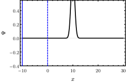
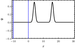
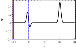
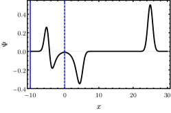
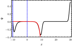
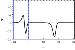
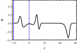
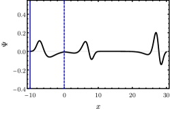
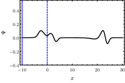
Figure 3 shows a ”time-lapse” of the complete waveform given by the sum of the open-system solution, Eq. (45), with the first 3 echoes, described by Eq. (III.2), with initial condition
| (57) |
and system parameters
| (58) |
The complete sequence of events can be seen in video format at: https://youtu.be/XfJNwuwbvnA .
III.3 QNMs
To substantiate the discussion at the end of the first section, let us compute the full system’s reflectivity. Usage of Eq. (II.5) with potential (40) yields
| (59) |
which simplifies to
| (60) |
by using the geometric series identity and definition of , Eq. (43).
It is easy to check that if and vice-versa, if then . Moreover, if , corresponding to a perfect mirror, then we should expect everything to be reflected back, independently of the potential. In this limit we can also see that .
More interestingly, at the delta QNM (44), , the dependence on cancels to give , which is finite for non-vanishing . Thus, is not a QNM of the mirror+delta system. The QNMs are instead implicitly given by
| (61) |
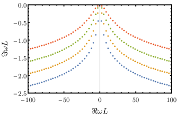
Fig. 1 plots the frequencies that respect the above, for given by Eq. (5), with (Dirichlet BC at ), which are well-approximated by the expression
| (62) |
Unsurprisingly, the imaginary part grows in magnitude with . This implies that, at sufficiently long times, the perturbation will decay with the fundamental mode (Fig. 2), even if the initial perturbation decays according to the pure-delta QNM (44) (as we show in Figure 3).
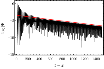
We believe that this is the most convincing demonstration to date that the late-time decay is indeed governed by the QNMs of the composite system.
 |
 |
 |
 |
 |
 |
 |
 |
 |
IV Final remarks
We have shown that a proper re-summation of the Dyson series solution of the Lippman-Schwinger equation accounts for the presence of echoes in the waveforms of extremely compact objects (termed “ClePhOs” in the nomenclature of Refs. Cardoso and Pani (2017a, b)). We recover previous results, obtained with a completely different approach Mark et al. (2017), but our approach also provides a few more insights.
The key result Eq.(II.3) besides confirming the lower frequency content, decaying amplitude and constant distance of successive echoes, also explicitly relates the echoes waveform with the initial conditions and sources incorporated into , the potential of the system , and the reflectivity of the wall (the latter two function as the right and left sides of the lossy cavity, respectively).
With the hypothetical future discovery of echoes in gravitational wave signals, the echo amplitude can be extracted up to experimental and numerical error. Together with the knowledge of and , this turns Eq. (II.3) into an equation for , which encodes the information we currently lack on the quantum structure at the event horizon.
Further developments of our formalism should include: application to other potentials besides the simple Dirac delta; a careful analysis of the convergence properties of Eq. (II.3); extension of our methods to more than one spatial dimension; check if superradiant amplification is observed in Eq. (II.3) if ; implementation of the reflectivity series (II.5) and (II.5) to QNM computation; confirm the polynomial behaviour of echoes in other systems besides the Dirac delta potential and use this information to echo modelling.
Acknowledgments. We thank José Natário for elucidating discussions and are grateful to Kinki university in Osaka for kind hospitality while part of this work was being completed. We acknowledge interesting discussions with the participants of the workshops “Physics and Astronomy at the eXtreme (PAX)” in Amsterdam and “Gravitational Dynamics and Black Holes” in Nagoya University. V.C. acknowledges financial support provided under the European Union’s H2020 ERC Consolidator Grant “Matter and strong-field gravity: New frontiers in Einstein’s theory” grant agreement no. MaGRaTh–646597. Research at Perimeter Institute is supported by the Government of Canada through Industry Canada and by the Province of Ontario through the Ministry of Economic Development Innovation. This article is based upon work from COST Action CA16104 “GWverse”, supported by COST (European Cooperation in Science and Technology). This work was partially supported by FCT-Portugal through the project IF/00293/2013, by the H2020-MSCA-RISE-2015 Grant No. StronGrHEP-690904.
References
- Cardoso and Gualtieri (2016) V. Cardoso and L. Gualtieri, Class. Quant. Grav. 33, 174001 (2016), arXiv:1607.03133.
- Cardoso and Pani (2017a) V. Cardoso and P. Pani, (2017a), arXiv:1707.03021.
- Berthiere et al. (2017) C. Berthiere, D. Sarkar, and S.N. Solodukhin, (2017), arXiv:1712.09914.
- Abbott et al. (2016a) B.P. Abbott et al. (The LIGO/Virgo Scientific Collaboration), Phys. Rev. Lett. 116, 061102 (2016a), arXiv:1602.03837.
- Abbott et al. (2016b) B.P. Abbott et al. (Virgo, LIGO Scientific), Phys. Rev. Lett. 116, 241103 (2016b), arXiv:1606.04855.
- Buonanno et al. (2007) A. Buonanno, G.B. Cook, and F. Pretorius, Phys. Rev. D75, 124018 (2007), arXiv:gr-qc/0610122.
- Berti et al. (2007) E. Berti, V. Cardoso, J.A. Gonzalez, U. Sperhake, M. Hannam, S. Husa, and B. Bruegmann, Phys. Rev. D76, 064034 (2007), arXiv:gr-qc/0703053.
- Sperhake et al. (2013) U. Sperhake, E. Berti, and V. Cardoso, Comptes Rendus Physique 14, 306 (2013), arXiv:1107.2819.
- Berti et al. (2009) E. Berti, V. Cardoso, and A.O. Starinets, Class. Quantum Grav. 26, 163001 (2009), arXiv:0905.2975.
- Blanchet (2014) L. Blanchet, Living Rev. Rel. 17, 2 (2014), arXiv:1310.1528.
- Abramowicz et al. (2002) M.A. Abramowicz, W. Kluzniak, and J.P. Lasota, Astron. Astrophys. 396, L31 (2002), arXiv:astro-ph/0207270.
- Krishnendu et al. (2017) N.V. Krishnendu, K.G. Arun, and C.K. Mishra, (2017), arXiv:1701.06318.
- Maselli et al. (2017a) A. Maselli, P. Pani, V. Cardoso, T. Abdelsalhin, L. Gualtieri, and V. Ferrari, (2017a), arXiv:1703.10612.
- Audley et al. (2017) H. Audley et al., (2017), arXiv:1702.00786.
- Flanagan and Hinderer (2008) E.E. Flanagan and T. Hinderer, Phys. Rev. D77, 021502 (2008), arXiv:0709.1915.
- Binnington and Poisson (2009) T. Binnington and E. Poisson, Phys. Rev. D80, 084018 (2009), arXiv:0906.1366.
- Damour and Nagar (2009) T. Damour and A. Nagar, Phys. Rev. D80, 084035 (2009), arXiv:0906.0096.
- Fang and Lovelace (2005) H. Fang and G. Lovelace, Phys. Rev. D72, 124016 (2005), arXiv:gr-qc/0505156.
- Gürlebeck (2015) N. Gürlebeck, Phys. Rev. Lett. 114, 151102 (2015), arXiv:1503.03240.
- Poisson (2015) E. Poisson, Phys. Rev. D91, 044004 (2015), arXiv:1411.4711.
- Pani et al. (2015) P. Pani, L. Gualtieri, A. Maselli, and V. Ferrari, Phys. Rev. D92, 024010 (2015), arXiv:1503.07365.
- Wade et al. (2013) M. Wade, J.D.E. Creighton, E. Ochsner, and A.B. Nielsen, Phys. Rev. D88, 083002 (2013), arXiv:1306.3901.
- Cardoso et al. (2017) V. Cardoso, E. Franzin, A. Maselli, P. Pani, and G. Raposo, Phys. Rev. D95, 084014 (2017), arXiv:1701.01116.
- Sennett et al. (2017) N. Sennett, T. Hinderer, J. Steinhoff, A. Buonanno, and S. Ossokine, (2017), arXiv:1704.08651.
- Berti et al. (2006) E. Berti, V. Cardoso, and C.M. Will, Phys. Rev. D73, 064030 (2006), arXiv:gr-qc/0512160.
- Berti et al. (2016) E. Berti, A. Sesana, E. Barausse, V. Cardoso, and K. Belczynski, Phys. Rev. Lett. 117, 101102 (2016), arXiv:1605.09286.
- Cardoso et al. (2016a) V. Cardoso, E. Franzin, and P. Pani, Phys. Rev. Lett. 116, 171101 (2016a), arXiv:1602.07309.
- Cardoso and Pani (2017b) V. Cardoso and P. Pani, Nat. Astron. 1, 586 (2017b), arXiv:1709.01525.
- Cardoso et al. (2016b) V. Cardoso, S. Hopper, C.F.B. Macedo, C. Palenzuela, and P. Pani, Phys. Rev. D94, 084031 (2016b), arXiv:1608.08637.
- Price and Khanna (2017) R.H. Price and G. Khanna, (2017), arXiv:1702.04833.
- Völkel and Kokkotas (2017a) S.H. Völkel and K.D. Kokkotas, Class. Quant. Grav. 34, 125006 (2017a), arXiv:1703.08156.
- Völkel and Kokkotas (2017b) S.H. Völkel and K.D. Kokkotas, (2017b), arXiv:1704.07517.
- Zhang and Zhou (2017) J. Zhang and S.Y. Zhou, (2017), arXiv:1709.07503.
- Abedi et al. (2016) J. Abedi, H. Dykaar, and N. Afshordi, (2016), arXiv:1612.00266.
- Abedi et al. (2017) J. Abedi, H. Dykaar, and N. Afshordi, (2017), arXiv:1701.03485.
- Ashton et al. (2016) G. Ashton, O. Birnholtz, M. Cabero, C. Capano, T. Dent, B. Krishnan, G.D. Meadors, A.B. Nielsen, A. Nitz, and J. Westerweck, (2016), arXiv:1612.05625.
- Westerweck et al. (2017) J. Westerweck, A. Nielsen, O. Fischer-Birnholtz, M. Cabero, C. Capano, T. Dent, B. Krishnan, G. Meadors, and A.H. Nitz, (2017), arXiv:1712.09966.
- Mark et al. (2017) Z. Mark, A. Zimmerman, S.M. Du, and Y. Chen, (2017), arXiv:1706.06155.
- Nakano et al. (2017) H. Nakano, N. Sago, H. Tagoshi, and T. Tanaka, PTEP 2017, 071E01 (2017), arXiv:1704.07175.
- Bueno et al. (2018) P. Bueno, P.A. Cano, F. Goelen, T. Hertog, and B. Vercnocke, Phys. Rev. D97, 024040 (2018), arXiv:1711.00391.
- Maselli et al. (2017b) A. Maselli, S.H. Völkel, and K.D. Kokkotas, Phys. Rev. D96, 064045 (2017b), arXiv:1708.02217.
- Wang et al. (2018) Y.T. Wang, Z.P. Li, J. Zhang, S.Y. Zhou, and Y.S. Piao, (2018), arXiv:1802.02003.
- Brito et al. (2015) R. Brito, V. Cardoso, and P. Pani, Lect. Notes Phys. 906, pp.1 (2015), arXiv:1501.06570.