Modal Decomposition of TTV - Inferring Planet Masses and Eccentricities
Abstract
Transit timing variations (TTVs) are a powerful tool for characterizing the properties of transiting exoplanets. However, inferring planet properties from the observed timing variations is a challenging task, which is usually addressed by extensive numerical searches. We propose a new, computationally inexpensive method for inverting TTV signals in a planetary system of two transiting planets. To the lowest order in planetary masses and eccentricities, TTVs can be expressed as a linear combination of 3 functions, which we call the TTV modes. These functions depend only on the planets’ linear ephemerides, and can be either constructed analytically, or by performing 3 orbital integrations of the three-body system. Given a TTV signal, the underlying physical parameters are found by decomposing the data as a sum of the TTV modes. We demonstrate the use of this method by inferring the mass and eccentricity of 6 Kepler planets that were previously characterized in other studies. Finally we discuss the implications and future prospects of our new method.
1 Introduction
When a transiting exoplanet is orbiting in the presence of a non-Keplerian potential, the timing of its transits may deviate from constant periodicity. Such deviations from linear ephemeris, known as transit timing variations (TTVs), possess valuable information regarding the perturbations to the Keplerian potential.
A primary source of TTVs is the presence of additional massive planets orbiting the same host star. TTVs were therefore recognized as a method for detecting non-transiting planets in planetary systems with at least one transiting planet and as a tool for confirming planet candidates (Miralda-Escudé, 2002; Agol et al., 2005; Holman & Murray, 2005; Nesvorný et al., 2012; Fabrycky et al., 2012).
TTVs can also serve as a proxy for constraining the masses and orbital parameters of the perturbing planets. When radial velocity measurements of the host star are not available, TTVs are the primary tool for constraining the mass (and bulk density) of transiting planets.
The Kepler mission has provided TTV measurements for hundreds of planets (Rowe et al., 2015; Holczer et al., 2016). Several authors have calculated planet masses and eccentricities of Kepler planets using the released data (Hadden & Lithwick, 2014, 2016, 2017; Lissauer et al., 2013). Most commonly, the inversion of TTVs for inferring planet properties is done using Markov chain Monte Carlo (MCMC) simulations (Hadden & Lithwick, 2016, 2017; Jontof-Hutter et al., 2016). MCMC simulations sample planet masses and orbital parameters, searching for the model most consistent with the observations. Typically these procedures require computation of - N-body orbital integrations, each lasting for a few hundreds of orbits (Deck et al., 2014). These intensive numerical searches are often complemented by fitting to approximate TTV formulae, that help in identifying the parameter degeneracies within the numerical searches (Hadden & Lithwick, 2016, 2017; Jontof-Hutter et al., 2016; Agol & Deck, 2016).
In this work, we propose a computationally inexpensive method for inferring planet properties from TTV signals of systems with two transiting planets. Assuming TTV amplitudes which are small compared to the orbital periods, low planet-to-star mass ratios and small orbital eccentricities, TTVs can be expressed as a linear sum of 3 dimensionless functions which we call the TTV modes. The TTV modes depend solely on the planets’ period ratio and orbital phase, which are known a-priori. We demonstrate how these modes can be easily constructed with merely 3 orbital integrations. Given a TTV signal, it can be decomposed to a sum of these modes, with coefficients that determine the unknown physical parameters of the perturbing planet.
Using data from TTV catalogs (Rowe et al., 2015; Holczer et al., 2016) we calculate the mass and eccentricity of 6 Kepler planets, (Kepler-307 b & c, Kepler-177 b & c, Kepler-11 d & e). The masses we infer are consistent with the values reported by previous works.
The outline of the paper is as follows. In section 2 we present the general form that TTVs take, and define the TTV modes. We discuss the procedure of fitting the modes and inferring the physical parameters in section 3. In section 4 we demonstrate the use of our method on a set of 6 Kepler planets. We discuss the interpretation of the TTV modes and compare them to other works in section 5. Finally, we discuss our conclusions and future prospects in section 6.
2 TTV Theory
2.1 Leading order TTV
Consider a planetary system with two transiting planets. Small mutual inclinations tend to have a negligible effect on TTVs (Nesvorný & Vokrouhlický, 2014; Hadden & Lithwick, 2016; Agol & Deck, 2016). Additionally, systems with multiple transiting planets have been observationally shown to be nearly coplanar, with typical mutual inclination of less than a few degrees (Figueira et al., 2012; Tremaine & Dong, 2012; Fabrycky et al., 2014). We will therefore assume that the two planets are on coplanar orbits. The TTVs of these planets depend on their masses and eccentricities. We define two small parameters, and , the relative masses of the inner and outer planet.
TTVs are insensitive to the individual eccentricities of the interacting planets, but rather to the combined free eccentricity vector (Lithwick et al., 2012; Hadden & Lithwick, 2016, 2017) - a weighted difference between the free-eccentricities of the two planets (see appendix A). The dependence of TTVs on this combined quantity rather than the individual eccentricities is known as the eccentricity-eccentricity degeneracy (see Lithwick et al. (2012); Jontof-Hutter et al. (2016) for further discussion).
One exception where this degeneracy may be lifted, is the case of proximity to the mean-motion resonance (MMR). A few studies have reported eccentricity measurements of individual planets in systems close to the MMR (Holman et al., 2010; Borsato et al., 2014). Excluding this case, TTVs strongly depend only on the system’s combined free eccentricity.
We define , the combined eccentricity component parallel to the observer’s line of sight, and , the component perpendicular to the observer (in the positive sense of rotation).
To the leading order in these small parameters, the TTV of the inner planet can be written in the following form
| (1) |
where , and are functions of the period ratio, and the angle between the planets at the time of the first transit, - both values are assumed to be known. We refer to these functions as the TTV modes. The TTV of the outer planet takes a similar functional form,
| (2) |
where , and are also functions of and . Note that the TTV of the inner planet depends on the mass of its perturbing companion, , and vice versa.
The general form TTVs take is given in equations 1 and 2. TTVs vanish when planetary masses go to zero, as the Keplerian orbits remain unperturbed. Since TTVs occur due to the gravitational interaction with a perturber, TTVs are expected to change linearly with mass, to lowest order, and hence the expressions are proportional to and .
TTVs depend mostly on the combined free eccentricity vector, rather than the individual eccentricities of the two planets. This behavior was shown both analytically and numerically by several authors (Hadden & Lithwick, 2016; Jontof-Hutter et al., 2016). Intuitively, this can be understood by the following argument. Assuming small individual eccentricities, an elliptical orbit, to first order in eccentricity, is given by a circle, with its center shifted by an amount proportional to its eccentricity, in the direction of its apocenter. Since the gravitational interaction between the planets depends on their relative positions, eccentricity enters through roughly as the difference in their eccentricity vectors. For instance, if two nearby planets have the same eccentricity vector, their relative motion will be along two concentric circular orbits, eliminating the effect of eccentricity.
The functions , and (and respectively, , and ) are linearly independent, and span the TTV space. Given the inner planet’s TTV signal , the unknown parameters , and can be uniquely determined by projecting onto the basis functions , and .
If the TTV signal contains no noise, the error in the parameter inference is strictly due to higher order terms not included in equation 1, , , etc. Since the planet to star mass ratios and orbital eccentricities are quite small, these will generally account for small corrections. An exception is when the planets are near a second-order MMR, where second-order terms in eccentricity dominate (see the TTV expressions in Hadden & Lithwick (2016, 2017) that account for higher order terms).
While the functions , and are linearly independent, they do not form an orthogonal basis. Therefore, using equation 1 to fit a noisy signal would result in correlated errors in the coefficients of the functions , and , and accordingly in the inferred physical parameters.
We note that when a system is near a first-order mean-motion resonance, and are nearly parallel (see for example figure 2). This results in the so-called mass-eccentricity degeneracy (Lithwick et al., 2012; Hadden & Lithwick, 2014, 2016). When the data is too noisy to disentangle the contributions of and , the strong correlation between and poses a difficulty in the parameter inference.
The TTV modes are easily obtained - either using analytical formulae or numerically, constructing the functions from a small number of N-body integrations (see section 2.2). The parameter inference problem reduces to finding the three parameters , and that minimize the error given the data samples. Since the theoretical TTV expression (right hand side of equation 1) is linear in , and , the best-fit parameters are obtained analytically through a single three-by-three matrix inversion (see section 3).
2.2 Constructing the TTV modes
The TTV modes, , and can be easily constructed by running 3 numerical orbital integrations. The modes are functions of and - the relative angular positions at the the time of first transit. Three N-body integrations are performed, all consistent with the target and . We set a small value for the two masses and . These masses have to be sufficiently small such that the TTVs are in the linear regime, yet large enough that the TTV signal is easily measured from the simulation. In practice we have used (). With these masses and phases, we run the following set of simulations, and measure the TTV for the inner planet:
-
1.
Both planets possess zero free-eccentricities. We denote the TTV of this simulation by .
-
2.
The inner planet has a small free-eccentricity , with the pericenter facing the observer, while the outer planet has zero free-eccentricity. We have used . We denote the TTV calculated from this simulation as .
-
3.
The inner planet has a small free-eccentricity , with the pericenter perpendicular to the observer, while the outer planet has zero free-eccentricity. We have used . We denote the TTV calculated from this simulation as .
Some of the intermediate transit indices may be missing from the observational data. Thus, when calculating the TTVs from the simulation results, we limit ourselves to the transit indices that appear in the data. Therefore, the modes also depend on the list of transit indices available in the data, rather than just and .
Note that setting the correct initial conditions that yield a specific free-eccentricity requires some care. In appendices A and B we provide an analytical expression for the resultant free-eccentricity as a function of the initial eccentricity.
Given these three synthetic TTV signals, we obtain the TTV modes:
| (3) |
| (4) |
| (5) |
where is the period of the inner planet in the numerical integration. The modes may be calculated with any set of three independent simulations, i.e., with different pericenter orientations. More generally, the TTV modes could also be calculated by running simulations. Then, for each separately, find the values of , & that best solve the set of equations (1), in the sense.
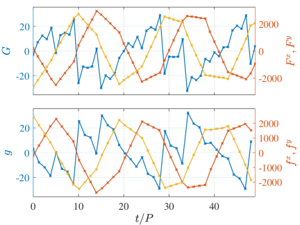
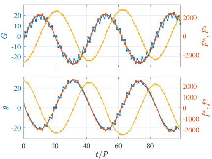
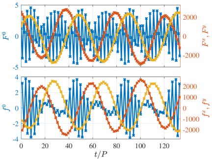
Figures 1 and 2 demonstrate the TTV modes associated with different period ratios, calculated using the above procedure. In figure 1, and . This orbital configuration lies between the the and MMRs.
Figure 2 demonstrates the TTV modes corresponding to a period ratio , and an initial angular separation . Due to system’s proximity to the MMR, the modes can be interpreted in terms of the TTV expressions of Hadden & Lithwick (2016, 2017) (see section 5 for further discussion on this comparison). and modes are roughly sinusoidal, slowly varying over the superperiod, similar to the ’fundamental’ TTV term (as defined in equation 1 of Hadden & Lithwick (2017)). The mode contains the ’chopping’ TTV term (see Deck & Agol (2015); Hadden & Lithwick (2016)), with a distinct synodic frequency. This figure also demonstrates the near-parallel nature of and . Up to their different scales, these modes are nearly identical, differing just by the high frequency component of .
3 Parameter inference using TTV modes
We distinguish between the known and unknown parameters that give rise to TTVs. The period of each planet, and the timing of its first transit are known by a linear fit to the list of transit times, i.e., the linear ephemeris. The planets’ masses and eccentricities are unknown and are to be inferred from the TTV signal. We describe our parameter inference procedure using the TTV modes.
-
1.
Perform a linear fit of the transit times to estimate the periods and . Given the (inner planet’s) transit times, , find and that minimize the error between the linear ephemeris, and the measurements, . Repeat for the outer planet, finding and .
-
2.
Given the constant terms in the linear fits, estimate , the angle between the planets, assuming circular orbits, at the time of the first transit.
- 3.
-
4.
We define the modes matrix
(6) where is the number of available transits in the data. If is the vector of TTV measurements,
(7) the physical parameters that minimize the error are given by
(8)
Step 3 is the most computationally expensive step in our TTV inversion procedure, as it involves 3 numerical orbital integrations. Nonetheless, our method is many orders of magnitude faster than the commonly used numerical methods for TTV inversion (Hadden & Lithwick, 2016), that require simulations. The orbital integrations we use in constructing the TTV modes can be calculated using TTVFast (Deck et al., 2014), which will expedite the computation times even further.
Given two TTV signals, the masses of both planets may be constrained ( from the TTV of the outer planet, and from inner planet’s TTV). The combined free-eccentricity is estimated separately from each planet’s TTVs. The eccentricity we finally report is given by the average of the two independent estimates, weighted by their corresponding error estimates.
Since the TTV modes are not orthogonal, the inferred physical parameters have correlated errors. As an example, consider a system with an orbital period ratio , whose corresponding TTV modes are shown in figure 2. When a noisy TTV signal is decomposed as a linear sum of , and , there is a strong degeneracy between the coefficients of and , as these modes are nearly parallel. If the higher frequency component of is not apparent in the data, and remain individually unconstrained. This is the so-called mass-eccentricity degeneracy, discussed in Lithwick et al. (2012); Wu & Lithwick (2013); Hadden & Lithwick (2014). When the signal-to-noise ratio is sufficiently high, the mode coefficients are properly constrained. In section 5.1 we discuss the orthogonalization of the TTV modes. This procedure highlights the difference between and , as shown in figure 7. The blue curve of figure 7 gives the high frequency component within the TTV signal that lifts the degeneracy between mass and eccentricity.
4 Results
| Planet | Period | Radius | Stellar Mass | Mass | Density | Ref. Mass | Ref. |
|---|---|---|---|---|---|---|---|
| [days] | [g/] | ||||||
| Kepler-307 b | 10.416 | Hadden & Lithwick (2017) | |||||
| Kepler-307 c | 13.084 | — | Hadden & Lithwick (2017) | ||||
| Kepler-177 b | 36.857 | Jontof-Hutter et al. (2016) | |||||
| Kepler-177 c | 49.411 | — | Jontof-Hutter et al. (2016) | ||||
| Kepler-11 d | 22.687 | Lissauer et al. (2013) | |||||
| Kepler-11 e | 31.995 | — | Lissauer et al. (2013) |
| Planet pair | Reference | ||
|---|---|---|---|
| Kepler-307 b & c | |||
| Kepler-177 b & c | |||
| Kepler-11 d & e |
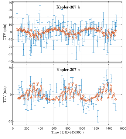
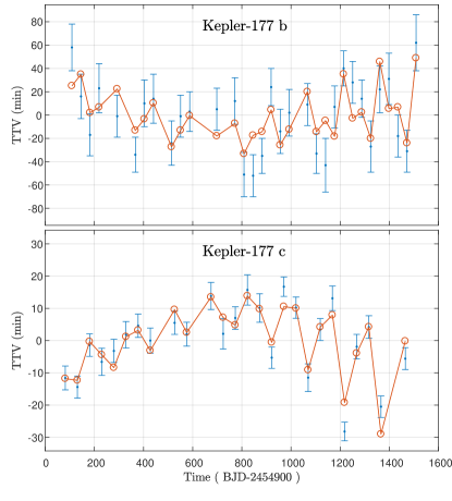
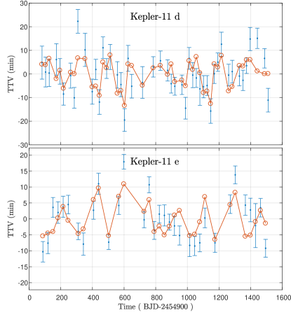
We demonstrate the use of our inversion method on a few Kepler planetary systems. The TTVs obtained from the catalogs of Holczer et al. (2016) and Rowe et al. (2015) for Kepler-307 (KOI-1576), Kepler-177 (KOI-523) and Kepler-11 (KOI-157) are shown in blue in figures 3, 4 and 5. The Holczer catalog uses the short-cadence data where available. The TTVs of all six planets (Kepler-307 b & c, Kepler-177 b & c, Kepler-11 d & e) are sufficiently accurate in order to confidently constrain planetary masses and eccentricities with the use of our method.
The red curve in figures 3 - 5 shows the signal reconstruction using the TTV modes that were calculated for each planet. This reconstruction is the linear combination of the three TTV modes that minimizes the squared differences with the TTV measurements.
The inferred planet masses and their densities are summarized in table 1. The masses we obtain for Kepler-307 b & c, and , are consistent with the values reported in Hadden & Lithwick (2017). Note that as they have used different values for the planet’s radii, the densities we find are inconsistent with theirs.
Figure 6 demonstrates the distributions of the physical parameters inferred for Kepler-307 b & c. The probability contours of these distributions show the correlation between the physical parameters. We marginalize these distributions and present the distributions of each parameter along the axis of this figure. We overlap the parameter distributions inferred from the TTV of both planets. Since TTVs are sensitive to the combined free-eccentricity, we find similar and values from the TTVs of both planets.
Having used the Holczer TTV catalog for Kepler-177 b & c, we find planetary masses consistent with those reported by Jontof-Hutter et al. (2016) when they have used the same TTV data. We find the masses of these planets, and . The bulk density we find for Kepler-177 c is outstandingly low, at about gr/cm3. This density is somewhat higher than the density reported by Hadden & Lithwick (2017), who use the long cadence Rowe catalog (Rowe et al., 2015), and higher than the density reported by Jontof-Hutter et al. (2016), who use slightly larger planet radius. Note that the fairly large uncertainties in the densities of Kepler-177 b & c (see table 1) are mostly due to the large uncertainties in the planetary radii, taken from the Exoplanet Archive.
Based on our analysis, Kepler-177 c has a surprisingly low bulk density, indicating the presence of a thick atmosphere, which is likely to dominate its volume (Lee & Chiang, 2016; Ginzburg et al., 2016). See further discussion regarding this planet in Jontof-Hutter et al. (2016)
The masses of Kepler-11’s six known planets were previously analyzed by Lissauer et al. (2013) using dynamical models. The masses and densities we report for Kepler-11 d & e, and , are in agreement with the uncertainty intervals of Lissauer et al. (2013).
Table 2 summarizes the inferred eccentricity we find for each of the systems. The combined free eccentricity is given by its magnitude, and its direction, . The angle is the argument of periapsis (of the the combined free eccentricity vector), measured with respect to the line of sight.
Note that both Kepler-307 and Kepler-177 are quite close to first-order MMR, resulting in a visually distinct sinusoidal feature in the TTV signal, varying on the superperiod in addition to the chopping signal (figures 3 and 4). See section 5 for more on the physical interpretation of the modes.
Planets Kepler-11 d & e are orbiting close to the second-order MMR. Near second order resonance, second-order terms in eccentricity dominate over the first-order eccentricity terms. Since our linear model does not include any terms, the eccentricity we infer for this system may be deemed inaccurate, since we assume linear dependence in eccentricity.
Kepler-11 is a system of 6 transiting planets. Nevertheless, we ignore the presence of the additional 4 planets in the analysis of Kepler 11 d & e. In principle, the TTV of these two planets may contain substantial contributions from the interaction with the additional planets, which we omit. In practice, if the planetary masses are similar and the planet pairs are away from MMR, the TTV is mostly determined by the neighboring planet with the closest orbital period.
5 Interpretation of the TTV modes
5.1 Mode orthogonalization
As discussed, the TTV modes as defined in equation 1 are generally not orthogonal. We note that in systems that are near a first-order MMR, the and modes are nearly parallel, as is well demonstrated in figure 2. One could orthogonalize the TTV modes using Gram-Schmidt process, to obtain an alternative set of modes.
In order to elucidate the structure of the TTV modes, we orthogonalize only and , by subtracting from its projection onto , and define
| (9) |
where
| (10) |
The general TTV expression (equation 1) then reads
| (11) |
5.2 Analogy to previous works
The form TTVs take (equation 11) is reminiscent of the analytical expression given by Hadden & Lithwick (2016, 2017). Yet, while Hadden & Lithwick (2016, 2017) derive their analytical formula under the assumption that the system is near a mean-motion resonance (MMR), the framework we adopt does not assume anything about proximity to MMR. We wish to highlight the mapping between our TTV expressions and the analytical results of Hadden & Lithwick (2017). Note that this mapping fails away from MMR, as their results apply only near MMR.
Hadden & Lithwick (2016, 2017) express a planet’s TTV as a sum of harmonic terms. They distinguish between three terms - ’fundamental’, ’chopping’, and ’secondary’ (see equation 1 of Hadden & Lithwick (2017) or equation 2 of Hadden & Lithwick (2016)).
The and modes are analogous to the ’fundamental’ TTV component defined in equations 1 and 2 of Hadden & Lithwick (2017). This is a sinusoidal term, whose amplitude increases as the system approaches a first-order MMR. It has the same period as the line of conjunctions period, called the superperiod. The contribution from and generally dominates when a system is near a first order mean-motion resonance. In this regime, and converge to sinusoidal functions whose period is the superperiod, sampled at the orbital frequency of the planet. The stripped-down TTV formula given in Lithwick et al. (2012), includes the fundamental component alone. Near resonance, and have a phase difference of roughly . Thus, the two amplitudes of these modes correspond to the amplitude and phase of the ’fundamental’ component.
is similar to the ’chopping’ TTV term, defined in equations 1 and 5 of Hadden & Lithwick (2017). The amplitude of this term varies smoothly with the period ratio , and does not diverge at quotients of small integers. It has a distinct synodic frequency. Expanded as a sum of frequency components, the chopping term as defined in Hadden & Lithwick (2017) excludes the ’fundamental’ frequency. This exclusion is analogous to the mode orthogonalization discussed in section 5.1.
Note that as we use a linear TTV model, our expression does not include an analog to the ’secondary’ component, which is a second-order term in eccentricity. The contribution of this term is important only at systems that are near a second-order mean-motion resonance.
6 Discussion
TTVs have been measured in a few hundreds of Kepler planets to date (Rowe et al., 2015; Holczer et al., 2016), and have been used to constrain the masses and eccentricities of a few dozens of planets (Hadden & Lithwick, 2017). Typically, this is done by using MCMC simulations, searching for the physical parameters most consistent with the observations.
We developed a new method for inverting TTV signals. This method is suited for systems with two transiting planets, with TTV amplitudes that are small compared to the orbital periods. In this regime, TTVs can be expressed as a linear sum of three known functions, accurate to first order in the combined eccentricity and planetary mass. These functions, or TTV modes, depend only on the transiting planets’ linear ephemerides, which are assumed to be known. Therefore, given a TTV signal, the mass and eccentricity are solved linearly, by decomposing the TTV signal as a sum of the TTV modes.
The modes can be easily constructed numerically, by running 3 orbital integrations of a 3-body system. The mode construction procedure incorporates the possibility of missing transits in the data. If some of the intermediate transit indices are missing, the modes are constructed using the existing indices alone. In this way we avoid systematic differences between the TTV template and the data, such as differences in the linear ephemerides being used.
We demonstrate the use of our method on 6 Kepler planets - Kepler-307 b & c, Kepler-177 b & c, Kepler-11 d & e using the TTV catalogs of Rowe et al. (2015) and Holczer et al. (2016). The masses and combined eccentricities we report are in agreement with masses previously reported by dynamical studies of these planetary systems (see table 1).
Our method solves the planetary masses and eccentricities linearly, as opposed to the computationally expensive MCMC simulations. Our approach is valid only in the linear regime, while the numerical calculations include all the additional higher order effects. However, since the planetary masses are small compared to with the stellar mass, and the typical eccentricities are also small, the linear terms are expected to dominate. A possible exception is when a system is near second-order MMR, where the first order terms in eccentricity vanish.
The parameters inferred from the TTV modes can also be used as an initial guess for numerical dynamical investigations. This may help expedite the convergence of MCMC simulations.
Our method is tailored for systems with two planets with measured TTVs. In this case, the TTV of the inner planet is approximated by the expression in equation 1. In the presence of higher multiplicity, the TTV of a given planet will generally depend on the masses and eccentricities of all other planets. As long as the linearity assumption is intact, the TTV of a given planet will be given by the linear sum of the pairwise TTV expressions, each calculated independently. Our method can be therefore extended to analyze the TTVs in systems with higher multiplicities.
Our approach utilizes the linearity of TTVs in order to easily infer the planets masses and eccentricities. The TTV modes can be constructed without the use of analytical formulas, simply by running 3 numerical simulations with arbitrary masses and eccentricities. Agol & Deck (2016) have provided an analytical TTV expression, accurate to first order in eccentricity (TTVFaster). This formula can be used in the construction of the TTV modes, which can then be used to infer the physical parameters of an observed system.
Appendix A Free eccentricities
The eccentricity vector of a perturbed planet can be written as
| (A1) |
where the forced eccentricity, is induced by the interaction with the companion planets. The free eccentricity, is constant on timescales shorter than the apsidal precession timescale. The eccentricity vector is pointed in the direction of the pericenter, at an angle , measured with respect to the observer’s line of sight.
The eccentricity that enters the TTV expressions is the combined free eccentricity. This eccentricity is a weighted difference between the two free eccentricity vectors of the outer and inner planets, with weights determined by the planets’ period ratio, . Different works have used somewhat different normalizations than the one we use (Lithwick et al., 2012; Hadden & Lithwick, 2016, 2017). In our paper, the combined free eccentricity is defined as
| (A2) |
where is an order-unity coefficient, which depends on . The value of can be found from the and coefficients listed in the tables of Lithwick et al. (2012); Hadden & Lithwick (2017). As noted in Hadden & Lithwick (2016, 2017), , hence the combined free eccentricity vector is roughly the difference between the planets’ eccentricities, .
Appendix B Initial conditions for a given free eccentricity
Consider two coplanar planets of masses , , periods and corresponding to the inner and outer planets, respectively. Assume that their initial angular positions are , , and that their initial eccentricities are and . Assuming that the free and forced eccentricities are small, and that , the free eccentricity is given by
| (B1) |
| (B2) |
where , and is a unit vector pointed at an angle
| (B3) |
and are function of , given by
| (B4) |
| (B5) |
References
- Agol et al. (2005) Agol, E., Steffen, J., Sari, R., & Clarkson, W. 2005, MNRAS, 359, 567
- Holman & Murray (2005) Holman, M. J., & Murray, N. W. 2005, Science, 307, 1288
- Holman et al. (2010) Holman, M. J., Fabrycky, D. C., Ragozzine, D., et al. 2010, Science, 330, 51
- Lithwick et al. (2012) Lithwick, Y., Xie, J., & Wu, Y. 2012, ApJ, 761, 122
- Wu & Lithwick (2013) Wu, Y., & Lithwick, Y. 2013, ApJ, 772, 74
- Hadden & Lithwick (2014) Hadden, S., & Lithwick, Y. 2014, ApJ, 787, 80
- Hadden & Lithwick (2016) Hadden, S., & Lithwick, Y. 2016, ApJ, 828, 44
- Hadden & Lithwick (2017) Hadden, S., & Lithwick, Y. 2017, AJ, 154, 5
- Nesvorný & Vokrouhlický (2014) Nesvorný, D., & Vokrouhlický, D. 2014, ApJ, 790, 58
- Deck & Agol (2015) Deck, K. M., & Agol, E. 2015, ApJ, 802, 116
- Agol & Deck (2016) Agol, E., & Deck, K. 2016, ApJ, 818, 177
- Deck et al. (2014) Deck, K. M., Agol, E., Holman, M. J., & Nesvorný, D. 2014, ApJ, 787, 132
- Nesvorný et al. (2012) Nesvorný, D., Kipping, D. M., Buchhave, L. A., et al. 2012, Science, 336, 1133
- Nesvorný et al. (2013) Nesvorný, D., Kipping, D., Terrell, D., et al. 2013, ApJ, 777, 3
- Nesvorný & Vokrouhlický (2014) Nesvorný, D., & Vokrouhlický, D. 2014, ApJ, 790, 58
- Holczer et al. (2016) Holczer, T., Mazeh, T., Nachmani, G., et al. 2016, ApJS, 225, 9
- Rowe et al. (2015) Rowe, J. F., Coughlin, J. L., Antoci, V., et al. 2015, ApJS, 217, 16
- Jontof-Hutter et al. (2016) Jontof-Hutter, D., Ford, E. B., Rowe, J. F., et al. 2016, ApJ, 820, 39
- Lissauer et al. (2013) Lissauer, J. J., Jontof-Hutter, D., Rowe, J. F., et al. 2013, ApJ, 770, 131
- Tremaine & Dong (2012) Tremaine, S., & Dong, S. 2012, AJ, 143, 94
- Figueira et al. (2012) Figueira, P., Marmier, M., Boué, G., et al. 2012, A&A, 541, A139
- Fabrycky et al. (2014) Fabrycky, D. C., Lissauer, J. J., Ragozzine, D., et al. 2014, ApJ, 790, 146
- Fabrycky et al. (2012) Fabrycky, D. C., Ford, E. B., Steffen, J. H., et al. 2012, ApJ, 750, 114
- Miralda-Escudé (2002) Miralda-Escudé, J. 2002, ApJ, 564, 1019
- Borsato et al. (2014) Borsato, L., Marzari, F., Nascimbeni, V., et al. 2014, A&A, 571, A38
- Lee & Chiang (2016) Lee, E. J., & Chiang, E. 2016, ApJ, 817, 90
- Ginzburg et al. (2016) Ginzburg, S., Schlichting, H. E., & Sari, R. 2016, ApJ, 825, 29