Generalized entropy formalism and a new holographic dark energy model

Abstract

Recently, the Rényi and Tsallis generalized entropies have extensively been used in order to study various cosmological and gravitational setups. Here, using a special type of generalized entropy, a generalization of both the Rényi and Tsallis entropy, together with holographic principle, we build a new model for holographic dark energy. Thereinafter, considering a flat FRW universe, filled by a pressureless component and the new obtained dark energy model, the evolution of cosmos has been investigated showing satisfactory results and behavior. In our model, the Hubble horizon plays the role of IR cutoff, and there is no mutual interaction between the cosmos components. Our results indicate that the generalized entropy formalism may open a new window to become more familiar with the nature of spacetime and its properties.

I Introduction

In standard cosmology, based on general relativity, one way to describe the current accelerating universe is to consider an unknown energy-momentum source called dark energy Roos ; Rev1 ; Rev2 . From thermodynamic point of view, dark energy candidates and horizon entropy can be affected by each other mswr ; em ; DEC37 ; ijtpmr ; pav . Recently, due to the unknown nature of spacetime, the long-range nature of gravity, and also motivated by the fact that the Bekenstein-Hawking entropy is a non-extensive entropy measure nn1 ; nn2 ; non2 ; non3 ; 5 , the Rényi and Tsallis generalized entropies nn1 ; nn2 ; nn3 ; non0 ; non1 ; abe ; 1 ; 2 ; fon ; 5 have been attributed to horizons to study various cosmological and gravitational phenomena non2 ; non15 ; non16 ; non17 ; non18 ; non19 ; non20 ; non21 ; non22 ; non23 ; non3 ; non13 ; non4 ; non5 ; non6 ; non7 ; non8 ; non9 ; non10 ; non11 ; non12 ; non14 ; eb ; eb1 ; 3 ; 4 ; 5 ; 6 ; 7 ; 8 ; 9 ; 10 ; 11 . The successes of these attempts in modelling the current accelerating cosmos non4 ; non5 ; non6 ; non7 ; non8 ; non9 ; non10 ; non14 ; non13 ; non19 ; non20 ; non21 encourage and motivate us to study the cosmos evolution in various generalized entropy setups which may help us to become familiar with the probable non-extensive features of spacetime, and thus its origin non20 .

Based on spacetime thermodynamics, the apparent horizon of FRW universe is a proper causal boundary Hay2 ; Hay22 ; Bak , meaning that the thermodynamics laws are satisfied on this boundary Cai2 ; CaiKim . Moreover, WMAP data indicates a flat FRW universe Roos , a universe for which apparent horizon is equal to the Hubble horizon. Thus, proper models of dark energy should be in agreement with the Hubble horizon in flat FRW background.

Following the Cohen et al’s hypothesis on the mutual relation between the UV cutoff and the entropy of system HDE , a new class of dark energy models have been proposed, called holographic dark energy (HDE) HDE01 ; HDE1 ; HDE2 ; HDE3 ; HDE4 ; HDES ; HDE5 ; HDE22 ; RevH ; wang . In flat FRW universe, the original model of HDE (OHDE) is constructed by attributing the Bekenstein-Hawking entropy to the cosmos horizon and also considering the Hubble horizon as its IR cutoff HDE01 ; HDE1 ; HDE2 ; HDE3 ; HDE4 ; HDES . Although the density parameter of OHDE shows an admissible behavior from itself, its energy density scales with $H^{2}$ meaning that it behaves as dark matter during the cosmos evolution HDE3 ; HDE4 , and in fact, OHDE is not in harmony with the Hubble radius HDE3 ; HDE4 . Besides, it is not always stable whenever it is dominant in cosmos and controls its expansion rate HDES . Due to such weaknesses of OHDE, various attempts have been made to modify this model RevH ; wang .

Although various entropies have been used to get modified HDE RevH ; wang , none of them consider the generalized entropy formalism to build a HDE model. As we have previously mentioned, the Rényi and Tsallis generalized entropies generate suitable models for the current universe, and thus, we are going to use such formalism to build a new model for HDE in flat FRW by considering the Hubble radius as its IR cutoff. Here, we use a special generalized entropy, a generalization of both the Rényi and Tsallis entropies, to build our model. In fact, our final aim of introducing this new holographic model is to show that the probable non-additive and non-extensive aspects of spacetime have theoretically enough potential to accelerate the universe in a consistent way with observations.

The paper is organized as follows. In the next section, after reviewing some generalized entropy formalisms, we introduce our model of HDE. In continue, we consider a non-interacting universe, for which there is no mutual interaction between the cosmos components, and study the evolution of system in Sec. (III). A summary on the present work is also presented in the last section. The unit of $c=\hbar=G=k_{B}=1$, where $k_{B}$ denotes the Boltzmann constant, has also been used in this paper.

II horizon entropy in generalized entropy formalism and holographic dark energy

Consider a system including $W$ states, in which $P_{i}$ is the probability of achieving the $i^{th}$ state satisfying the $\sum_{i=1}^{W}P_{i}=1$ condition. In this manner, Shannon’s entropy can be employed to build ordinary statistical mechanics and its corresponding thermodynamics in which additivity and extensivity are the backbone of all results. Some systems, such as those including long range interactions, do not necessarily preserve the additivity and extensivity properties nn1 ; nn2 ; nn3 ; non0 ; non1 ; abe ; 1 ; 2 ; fon . These are generally the systems described better by a power law distribution of probabilities, namely $P_{i}^{Q}$ where $Q$ is a real parameter pla , instead of the ordinary $P_{i}$ distribution meaning that other entropy measures are needed to describe these systems non0 ; non1 ; SM1 ; SM2 ; pla .

Rényi ($\mathcal{S}$) and Tsallis ($S_{T}$) entropies are two well-known of one-parameter generalized entropy defined as nn3 ; non0 ; non1

$$\mathcal{S}=\frac{1}{\delta}\ln\sum_{i=1}^{W}P_{i}^{1-\delta},$$ (1)

$$S_{T}=\frac{1}{\delta}\sum_{i=1}^{W}\left(P_{i}^{1-\delta}-P_{i}\right),$$

where $\delta\equiv 1-Q$. Combining the above one-parametric entropy measures with each other, we can find their mutual relation nn3 ; non0 ; non1 ; non19 ; non20

$$\mathcal{S}=\frac{1}{\delta}\ln(1+\delta S_{T}).$$ (2)

There is also another generalized entropy measure, introduced by Sharma and Mittal SM1 ; SM2 , indeed a two-parametric entropy defined as pla ; SM1 ; SM2 ; SM3 ; SM4 ; SM5

$$S_{SM}=\frac{1}{1-r}\big{(}(\sum_{i=1}^{W}P_{i}^{1-\delta})^{\frac{1-r}{\delta}}-1\big{)},$$ (3)

where $r$ is a new free parameter. Some basic properties of this entropy are addressed in Refs. pla ; SM1 ; SM2 ; SM3 ; SM4 ; SM5 which show its compatibility with various systems and indicate that it is a generalization of both the Rényi and Tsallis entropy. In fact, we can see that the Rényi and Tsallis entropies are recovered at the appropriate limits of $r\rightarrow 1$ and $r\rightarrow 1-\delta=Q$, respectively pla ; SM1 ; SM2 ; SM3 ; SM4 ; SM5 . Using Eqs. (1) and (3), one can easily reach

$$S_{SM}=\frac{1}{R}\big{(}(1+\delta S_{T})^{\frac{R}{\delta}}-1\big{)},$$ (4)

where $R\equiv 1-r$.

As we mentioned, systems including the long-range interactions are better described by generalized entropies based on the power law distributions of probability 1 ; 2 ; pla ; fon . Gravity is also a long-range interaction which motivates physicist to use the Rényi and Tsallis generalized entropies in order to study the gravitational and cosmological systems non2 ; non15 ; non16 ; non17 ; non18 ; non19 ; non20 ; non21 ; non22 ; non23 ; non3 ; non13 ; non4 ; non5 ; non6 ; non7 ; non8 ; non9 ; non10 ; non11 ; non12 ; non14 ; eb ; eb1 ; 3 ; 4 ; 5 ; 6 ; 7 ; 8 ; 9 ; 10 ; 11 . Since $S_{SM}$ is the generalized form of both $\mathcal{S}$ and $S_{T}$ pla ; SM1 ; SM2 ; SM3 ; SM4 ; SM5 , we use $S_{SM}$ to build a new HDE.

It has recently been argued that the Bekenstein-Hawking is a proper candidate for the Tsallis entropy abe ; non2 ; non3 ; 5 ; non18 ; non19 ; non20 ; non21 ; non22 ; non23 allowing us to replace $S_{T}$ with $S_{B}$ in the above equation which leads to

$$S_{SM}=\frac{1}{R}\big{(}(1+\frac{\delta A}{4})^{\frac{R}{\delta}}-1\big{)},$$ (5)

for the Sharma-Mittal entropy. In order to obtain this result, we also used $S_{B}=\frac{A}{4}$, where $A$ is the horizon area. For example, the Bekenstein-Hawking entropy is obtained by using the Tsallis formalism in order to calculate the entropy of black holes in loop quantum gravity 5 . Thus, bearing Eq. (4) in mind, we can say that Eq. (5) is in fact the Sharma-Mittal entropy content of system.

Sharma-Mitall Holographic Dark Energy (SMHDE)

Based on the holographic principle, the IR ($L$) and UV ($\Lambda$) cutoffs are in relation with the system horizon ($S$) as HDE5 ; HDE4

$$\Lambda^{4}\propto\frac{S}{L^{4}},$$ (6)

In HDE hypothesis, the zero-point energy density ($\rho_{\Lambda}$) corresponding to the cut-off $\Lambda$ ( $\rho_{\Lambda}\sim\Lambda^{4}$), plays the role of the energy density of dark energy ($\rho_{D}$) meaning that we have $\rho_{D}\sim\Lambda^{4}$HDE5 ; HDE4 . Now, considering the Hubble radius as the IR cutoff leading to $L\equiv H^{-1}=\sqrt{\frac{A}{4\pi}}$, and by using Eqs. (5) and (6), we reach at

$$\rho_{D}=\frac{3C^{2}H^{4}}{8\pi R}[(1+\frac{\delta\pi}{H^{2}})^{\frac{R}{\delta}}-1].$$ (7)

Here, $C^{2}$ is the unknown free parameter as usual, for the energy density of SMHDE. The original HDE model is also obtainable at the appropriate limit of $R\rightarrow\delta$. Here, we consider a setup in which there is no interaction between various components of cosmos, meaning that SMHDE obeys ordinary conservation law, and thus

$$p_{D}=-(\frac{\dot{\rho}_{D}}{3H}+\rho_{D})=-(\frac{\rho_{D}^{\prime}\dot{H}}{3H}+\rho_{D}),$$ (8)

where $\rho^{\prime}=\frac{d\rho_{D}}{dH}$, and dot denotes derivative with respect to time.

III Universe evolution

In a flat FRW universe, Friedmann equations are

$$H^{2}=\frac{8\pi}{3}(\rho_{m}+\rho_{D}),$$ (9)

$$H^{2}+\frac{2}{3}\dot{H}=\frac{-8\pi}{3}(p_{D}),$$

where $\rho_{m}=\rho_{0}a^{-3}$ and $\rho_{0}$ denote energy density of matter fields, and its value at the current era ($a=1$), respectively. One can also obtain $p_{D}$ as a function of $H$, by combining Eqs. (7) and (8) with the second Friedmann (9).

Now, defining $H^{2}(z)=E^{2}(z)H^{2}_{0}$, where $H_{0}$ is the current value of the Hubble parameter, and $\Omega_{m}=\frac{\rho_{0}}{\frac{3H_{0}^{2}}{8\pi}}$, Eq. (9) can be rewritten as

$$E^{2}(z) = \Omega_{m}(1+z)^{3}$$

$$+ \frac{\frac{3C^{2}H_{0}^{4}E^{4}(z)}{8\pi R}[(1+\frac{\delta\pi}{H_{0}^{2}E^{2}(z)})^{\frac{R}{\delta}}-1]}{\frac{3H_{0}^{2}}{8\pi}},$$

which finally leads to

$$E^{2}(z)=$$ (11)

$$\Omega_{m}(1+z)^{3}+\frac{(1-\Omega_{m})E^{4}(z)}{[(1+\frac{\delta\pi}{H_{0}^{2}})^{\gamma}-1]}[(1+\frac{\delta\pi}{H_{0}^{2}E^{2}(z)})^{\gamma}-1],$$

where $\gamma\equiv\frac{R}{\delta}$. In obtaining the above equation, we used the $E(z=0)=1$ condition which leads to

$$\frac{C^{2}H_{0}^{2}}{R}=\frac{1-\Omega_{m}}{[(1+\frac{\delta\pi}{H_{0}^{2}})^{\frac{R}{\delta}}-1]}.$$ (12)

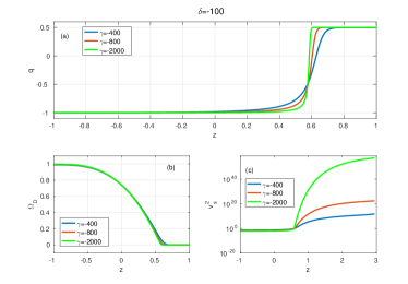
Figure 1: $q$, $\Omega_{D}(z)$ and $v_{s}^{2}(z)$ versus $z$ for some values of $\gamma$. Here, $\delta=-100$, $\Omega_{m}=0\cdot 26$ and $H_{0}=67\ (Km/s)/Mpc$.

The deceleration parameter is also evaluated as

$$q=-1+\frac{1+z}{E(z)}\frac{dE(z)}{dz}.$$ (13)

Moreover, since the density parameter of SMHDE is defined as $\Omega_{D}(z)=\frac{\rho_{D}}{\frac{3H_{0}^{2}}{8\pi}}$, we obtain

$$\Omega_{D}(z)=\frac{(1-\Omega_{m})E^{4}(z)}{[(1+\frac{\delta\pi}{H_{0}^{2}})^{\gamma}-1]}[(1+\frac{\delta\pi}{H_{0}^{2}E^{2}(z)})^{\gamma}-1],$$ (14)

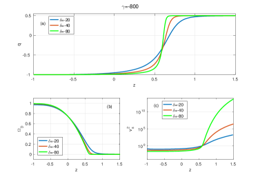
Figure 2: $q$, $\Omega_{D}(z)$ and $v_{s}^{2}(z)$ versus $z$ for some values of $\delta$. Here, $\gamma=-800$, $\Omega_{m}=0\cdot 26$ and $H_{0}=67\ (Km/s)/Mpc$.

leading to $\Omega_{D}(z=0)=1-\Omega_{m}$ for current era, a desired result. By inserting $\dot{H}=-4\pi p_{D}-\frac{3H^{2}}{2}$ and Eq. (14) into Eq. (8), the pressure of SMHDE is calculated as

$$p_{D}=\frac{\rho_{D}-\frac{E(z)}{2}\frac{d\rho_{D}}{dE(z)}}{(\frac{4\pi}{3H_{0}^{2}E(z)})\frac{d\rho_{D}}{dE(z)}-1},$$ (15)

which can be used in order to study the stability of system at classical level determined by the sign of the sound velocity evaluated as

$$v_{s}^{2}(z)=\frac{dp_{D}}{d\rho_{D}}=\frac{\frac{dp_{D}}{dz}}{\frac{d\rho_{D}}{dz}}=\frac{\frac{dp_{D}}{dE(z)}}{\frac{d\rho_{D}}{dE(z)}}.$$ (16)

In fact, whenever $v_{s}^{2}(z)$ is positive, SMHDE is stable.

In Figs. (1) and (2), we have plotted $q$, $\Omega_{D}(z)$ and $v_{s}^{2}(z)$ versus $z$ for some values of $\gamma$ and $\delta$. From the panels ($a$) and ($b$) of both figures, we see that there is a redshift ($z_{d}$) for which $q\simeq\frac{1}{2}$ and $\Omega_{D}(z)\simeq 0$, and its value is increased at a fixed $\delta$ ($\gamma$), by increasing the value of $\gamma$ ($\delta$). Moreover, panels ($c$) indicate that SMHDE is stable for $z<z_{d}$ and changes in $v_{s}^{2}(z)$ will be more relaxed by increasing the value of $\gamma$ ($\delta$) at a fixed $\delta$ ($\gamma$). Indeed, $v_{s}^{2}(z)$ has a singularity at $z=z_{d}$ and will be negative for $z>z_{d}$, meaning that such dark energy candidate cannot remain stable in the matter dominated era, and thus, the probable non-extensive features of spacetime cannot affect and accelerate the universe expansion for $z>z_{d}$. Therefore, our model may show better stability against the OHDE constructed by considering Bekenstein-Hawking entropy and Hubble horizon as its IR cutoff HDES .

The transition redshift ($z_{t}$), for which $q=0$, has also been plotted in Fig. (3) for some values of $\delta$ and $\gamma$ (panels ($a$) and ($c$)) that lead to results compatible with the $0\cdot 55\leq z_{t}\leq 0\cdot 8$ range. Hence, this model can theoretically produce proper values for $z_{t}$ Roos ; RevH ; wang ; HDE5 . It is useful to note here that since $\gamma$ and $\delta$ are negative, $R$ is positive in full agreement with Eqs. (12), (7) and thus the behavior of $\Omega_{D}(z)$. In panels ($b$) and ($d$) of Fig. (3), some values of $\delta$ and $\gamma$ have been shown for them the current value of the deceleration parameter ($q_{0}$) is within into the proper range of $-0\cdot 55\leq q_{0}\leq-1$ Roos .

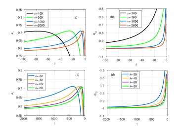
Figure 3: $z_{t}$ and $q_{0}$ for some values of $\delta$ and $\gamma$, whenever $\Omega_{m}=0\cdot 26$ and $H_{0}=67\ (Km/s)/Mpc$.

Finally, it is worthwhile mentioning that the total state parameter defined as $w\equiv\frac{p_{D}}{\rho_{D}+\rho_{m}}$ can be combined with Eq. (13) and (9) to reach at

$$w=\frac{2}{3}(q-\frac{1}{2}).$$ (17)

Comparing this equation with the behavior of $q$ and $q_{0}$, plotted in Figs. (1), (2) and (3), one can see that $w$ has proper behavior during the universe expansion in our model from matter dominated era ($w=0$), in which $q=\frac{1}{2}$, to the current era ($w\leq-\frac{2}{3}$), for which $q\leq-0\cdot 55$ Roos . In addition, we can see that, at the $z\rightarrow-1$ limit since $q\rightarrow-1$, our model predicts $w\rightarrow-1$. Finally, as it is apparent from Fig. (3), we should note here that there are wide ranges for $\delta$ and $\gamma$ which can produce desired results.

IV Conclusion

Attributing the Sharma-Mitall entropy to the horizon of flat FRW universe, accepting the Bekenstein-Hawking entropy as the Tsallis entropy, and by employing the holographic principle, we obtained a HDE (SMHDE) in which Hubble horizon, in agreement with the thermodynamics of flat FRW spacetime Hay2 ; Hay22 ; Bak ; CaiKim ; Cai2 , plays the role of IR cutoff. In addition, the evolution of universe filled by a pressureless component and SMHDE, which do not have any mutual interaction, has analytically been studied. Our approach shows that this model may theoretically meet primary requirements to model the cosmos expansion history. Therefore, our investigation offers that the generalized statistical mechanics and its corresponding thermodynamics have theoretically enough power to be in an acceptable agreement with the behavior of cosmos motivating us to more study the probable non-extensive aspects of spacetime.