Theory of open quantum dynamics with hybrid noise

Abstract

We develop a theory to describe dynamics of a non-stationary open quantum system interacting with a hybrid environment, which includes high-frequency and low-frequency noise components. One part of the system-bath interaction is treated in a perturbative manner, whereas the other part is considered exactly. This approach allows us to derive a set of master equations where the relaxation rates are expressed as convolutions of the Bloch-Redfield and Marcus formulas. Our theory enables analysis of systems that have extremely small energy gaps in the presence of a realistic environment. As an illustration, we apply the theory to the 16-qubit quantum annealing problem with dangling qubits and show good agreement with experimental results.

I Introduction

The theory of open quantum dynamics Leggett87 ; Slichter90 ; Walls94 is an important and active area of physics with applications in nanotechnology, chemical physics, quantum biology, and quantum information. In open quantum theories, the system under consideration is assumed to interact with an environment that has many degrees of freedom. Because details of the environmental Hamiltonian are usually unknown, measurable quantities such as temperature $T$ or noise spectrum $S(\omega)$ are used to describe the average statistical behavior of the environment. An open quantum model, therefore, provides a set of differential equations that describe the statistical dynamics of the quantum system, taking the temperature and the spectrum of the bath as input parameters.

Increased research and development of technology in quantum computing is renewing interest in open quantum modeling. One such promising computation scheme is quantum annealing (QA) Kadowaki98 ; Santoro02 ; Johnson11 (in particular, adiabatic quantum computation Farhi01 ). In QA, the system is evolved slowly so that it stays at or near the ground state throughout the evolution. At the end of the evolution, the system will occupy a low-energy state of the final Hamiltonian, which may represent a solution to an optimization or a sampling problem.

Open quantum dynamics of a QA processor have been studied theoretically Sahel06 ; AminLove ; Albash12 ; Albash15 . These models assume weak coupling to an environment, which is typically taken to have Ohmic spectrum with large high-frequency content. This limit is well described by the Bloch-Redfield theory Leggett87 ; Slichter90 ; Walls94 ; AminLove ; ES81 . Realistic qubits Harris10 , however, suffer from strong interaction with low-frequency noise (in particular, noise with 1/f-like spectrum). Incoherent dynamics of a qubit coupled to such an environment are described by the Marcus theory Marcus93 ; Cherepanov01 ; LNT17 . A complete (hybrid) open quantum model should account for both low-frequency and high-frequency environments. Such a model for a single qubit has been developed and agreement with experiment has been demonstrated Amin08 ; AminBrito09 ; Lanting11 . A generalization of this theory to multiqubit systems has also been developed and compared with experimental observation Boixo16 ; Boixo14 . Several attempts to combine the Bloch-Redfield and Marcus methods have been undertaken in chemical physics and quantum biology(see, for example, Refs.Yang02 ; Ghosh11 ; Lambert13 ).

In this paper, we expand the work of Refs. Boixo16 ; Boixo14 . We provide a systematic and detailed derivation of a hybrid open quantum model, which agrees with the results of Ref. Boixo16 ; Boixo14 for problems with large spectral gaps. Our theory, however, can also be applied to small-gap problems with nonstationary Hamiltonians, for which the model in Boixo16 ; Boixo14 is not applicable. We provide an intuitively appealing and computationally convenient form for the transition rates in terms of a convolution between Redfield and Marcus formulas. As an example, we investigate a dissipative evolution of a 16-qubit system strongly interacting with low-frequency noise and weakly coupled to a high-frequency environment. The problem is characterized by an extremely small gap in the energy spectrum of qubits in the middle of annealing. Solving the problem requires the right combination of Bloch-Redfield and Marcus approaches as well as a proper consideration of the calculation basis, which takes into account the nonstationary effects. The results of the present paper can also be applied to any other open quantum system.

The paper is organized in the following way. Section II describes a single-qubit system to provide the necessary intuition before moving to more complicated multi-qubit problems. Section III formulates the Hamiltonian and introduces important definitions and notations for the system and the bath. Master equations for the probability distribution of the quantum system are derived in Section IV. Section V presents the relaxation rates as convolution integrals of the Bloch-Redfield and Marcus envelopes. In the Section VI we show that in equilibrium the master equations obey the detailed balance conditions. We also demonstrate that the convolution expression for the relaxation rates turns into the Marcus or to Bloch-Redfield formulas in the corresponding limits. Dissipative dynamics of a 16-qubit system with an extremely small energy gap is considered in Section VII. A brief compilation of the commonly encountered notations is presented in Appendix A. In other Appendixes we provide a detailed derivation of many important formulas.

II Single-qubit system

We begin with a single-qubit system that has a Hamiltonian

$$H_{S}=-\frac{\Delta}{2}\,\sigma_{x}-\frac{h}{2}\,\sigma_{z},$$ (1)

with the Pauli matrices $\sigma_{x},\sigma_{y},\sigma_{z}$, tunneling amplitude $\Delta$, and bias $h$. The ground state, $|1\rangle$, and the excited state, $|2\rangle$, of the Hamiltonian (1) have energies $E_{1,2}=\mp\frac{\Omega_{0}}{2}$, with the energy splitting $\Omega_{0}=\sqrt{\Delta^{2}+h^{2}}.$ We assume that the system-bath interaction is determined by the Hamiltonian

$$H_{\rm int}=-Q\,\sigma_{z},$$ (2)

where $Q$ is a quantum-mechanical operator of the bath. The bath itself has a Hamiltonian $H_{B}$, so that the total Hamiltonian $H$ of the problem is a sum of three terms:

$$H=H_{S}+H_{\rm int}+H_{B}.$$ (3)

We assume that the free bath (with no coupling to the system) has a Gaussian statistics ES81 determined by a spectrum of fluctuations:

$$S(\omega)=\int dte^{i\omega t}\langle Q(t)Q(0)\rangle,$$ (4)

where $Q(t)=e^{iH_{B}t}Qe^{-iH_{B}t}$. Frequently, the Gaussian bath is represented as a collection of harmonic oscillators Leggett87 . Within our general formalism we do not have to resort to any specific representation of the bath.

In many realistic situations (see, for example, Refs. Lanting11 ), the noise may come from different sources, some dominating at low frequencies (such as 1/f noise) and others dominating at high frequencies. As such, we consider $S(\omega)$ to be a sum of two terms:

$$S(\omega)~{}=~{}S_{L}(\omega)~{}+~{}S_{H}(\omega),$$ (5)

where $S_{L}(\omega)$ and $S_{H}(\omega)$ are functions that are peaked at low and high frequencies, respectively. Each function may tail into the other function’s region. Hereafter we refer to the noise with the spectrum (5) as the hybrid noise. The formula of high-frequency spectrum $S_{H}$ is given in Sec. III E. For the explicit expression for $S_{L}(\omega)$ we refer to Eq. (B3) shown in the Supplementary Information Section of Ref. Johnson11 , although there are no need for these formulas here. Notice also that in the present paper we operate with the experimentally-measured parameters of the low-frequency bath, such as the noise intensity $W^{2}$ and the reorganization energy $\varepsilon_{L}$, which are are defined below.

The relaxation dynamics of the qubit become simple in two situations. First, when the qubit is weakly coupled to only a high-frequency (HF) bath and the energy splitting of the qubit is larger than the broadening of qubit’s energy levels. In this case, the relaxation is described by the Bloch-Redfield rate Leggett87 ; Slichter90 ; Walls94 ,

$$\Gamma=\frac{\Delta^{2}}{\Delta^{2}+h^{2}}\,S_{H}(\Omega_{0}),$$ (6)

which is valid when $\Gamma\ll\Omega_{0}$. Herein, we make the following assumptions for the Boltzmann and Planck constants: $k_{B}=1,\;\hbar=1.$

The second case is when the qubit is coupled only to a low-frequency (LF) bath and its tunneling amplitude is much smaller than the energy broadening caused by noise. The qubit dynamics therefore becomes incoherent and the resulting macroscopic resonant tunneling (MRT) rate is given by Amin08 ; AminBrito09

$$\Gamma=\frac{\Delta^{2}}{8}\,\sqrt{\frac{2\pi}{W^{2}}}\,\exp\left[-\frac{(h-4\,\varepsilon_{L})^{2}}{8W^{2}}\right],$$ (7)

where

$$W^{2}=\int\frac{d\omega}{2\pi}S_{L}(\omega),\;\;\varepsilon_{L}=\int\frac{d\omega}{2\pi}\frac{S_{L}(\omega)}{\omega}$$ (8)

determine the intensity of the noise and the reorganization energy (the shift of the bath energy due to the change of the qubit state), respectively. The fluctuation-dissipation theorem leads to $W^{2}=2\,\varepsilon_{L}\,T,$ where $T$ is the equilibrium temperature of the bath Amin08 . Equation (7), commonly known as the Marcus formula Marcus93 ; Cherepanov01 ; Yang02 ; Ghosh11 , is valid when the tunneling amplitude $\Delta$ is much smaller than the MRT line-width $W$: $\Delta\ll W.$ This equation has been successful in explaining experimental data from flux qubits Lanting11 ; Harris08 .

In practice, low and high-frequency noises coexist and both have to be considered in the dynamics of the qubit. In Refs. Lanting11 ; Amin08 the formula (7) has been generalized to include effects of high-frequency noise on the MRT rate. For small tunneling amplitudes $\Delta$ the modified rate $\Gamma$ is described by the following integral:

$$\Gamma=\frac{\Delta^{2}}{4}\,\int d\tau\;e^{i(h-4\varepsilon_{L})\tau-2W^{2}\tau^{2}}\times$$

$$\exp\left[4\int\frac{d\omega}{2\pi}\,\frac{S_{H}(\omega)}{\omega^{2}}\,\left(e^{-i\omega\tau}-1\right)\right].$$ (9)

We notice that the integrand of Eq. (II) is equal to the product of the low-frequency component, $e^{-2W^{2}\tau^{2}-4i\varepsilon_{L}\tau}$, multiplied by the high-frequency factor, which depends on the spectrum $S_{H}$. The low-frequency component has the Gaussian Fourier image,

$$G^{L}(\omega)=\sqrt{\frac{\pi}{2W^{2}}}\,\exp\left[-\frac{(\omega-4\varepsilon_{L})^{2}}{8W^{2}}\right].$$ (10)

The high-frequency factor is characterized by the more complicated integral:

$$G^{H}(\omega)=\int_{-\infty}^{+\infty}d\tau\;e^{i\omega\tau}\times$$

$$\exp\left[4\int\frac{d\Omega}{2\pi}\,\frac{S_{H}(\Omega)}{\Omega^{2}}\,\left(e^{-i\Omega\tau}-1\right)\,\right].$$ (11)

We notice that both functions, $G^{L}(\omega)$ and $G^{H}(\omega)$, satisfy the normalization condition,

$$\int\frac{d\omega}{2\pi}\,G^{\mu}(\omega)=1,$$ (12)

where $\mu=L,H.$

The rate (II) can be represented as a convolution of the Gaussian envelope $G^{L}(\omega)$ and the function $G^{H}(\omega)$,

$$\Gamma=\frac{\Delta^{2}}{4}\,\int\frac{d\omega}{2\pi}\,G^{L}(h-\omega)\,G^{H}(\omega).$$ (13)

In the Markovian case, where the spectrum $S_{H}(\omega)$ is flat, $S_{H}(\omega)=S_{H}(0)$, the function $G^{H}(\omega)$ has a Lorentzian shape,

$$G^{H}(\omega)=\frac{4S_{H}(0)}{\omega^{2}+[2S_{H}(0)]^{2}}.$$ (14)

Here we need not to assume that the qubit-bath coupling is small. Equation (14) is valid at frequencies $0\leq\omega\leq 1/\tau_{H},$ where $\tau_{H}$ is a correlation time of the high-frequency fluctuations described by the function $S_{H}(\omega).$ Later we introduce a spectral density $S_{H}$ of the Ohmic noise characterized by the correlation time $\tau_{H}\sim 1/T.$

The Bloch-Redfield limit is described by Eq. (II) with the frequency $\omega$, which is much larger than the coupling to the environment given by the spectrum $S_{H}(\omega)$: $\frac{S_{H}(\omega)}{\omega}\ll 1.$ With this small parameter, we can expand the dissipative factor in Eq. (II). Now the function $G^{H}(\omega)$ turns into the form

$$G^{H}(\omega)=4\frac{S_{H}(\omega)}{\omega^{2}}.$$ (15)

Equations (14) and (15) can be approximately combined into one Lorentzian formula that has a frequency-dependent numerator,

$$G^{H}(\omega)=\frac{4S_{H}(\omega)}{\omega^{2}+[2S_{H}(0)]^{2}}.$$ (16)

The Markovian and Bloch-Redfield expressions follow from this formula in the corresponding limits. Notice also that the function (16) is normalized according to Eq. (12).

Thus, the single-qubit relaxation rate (II) can be conveniently represented as a convolution of the Gaussian and Lorentzian line shapes,

$$\Gamma=\frac{\Delta^{2}}{4}\,\int\frac{d\omega}{2\pi}\,\frac{S_{H}(\omega)}{\omega^{2}+[2S_{H}(0)]^{2}}\times$$

$$\sqrt{\frac{\pi}{2W^{2}}}\,\exp\left[-\frac{(h-\omega-4\varepsilon_{L})^{2}}{8W^{2}}\right].$$ (17)

The convolution integral in (II) has a simple interpretation. One can think of the low-frequency noise as a random shift in energy bias: $h\to h+h_{\rm noise}$, where $h_{\rm noise}$ has Gaussian distribution with variance of $2W$. The high-frequency relaxation rate, given by the Lorentzian line-shape, will therefore be shifted by $h_{\rm noise}$. Ensemble averaging over low-frequency fluctuations will lead to a convolution integral similar to (13) and (II). The reorganization energy $\varepsilon_{L}$ is a result of the action of the qubit on the environment.

The intuitive description above holds beyond the validity of Eq. (II). In the next sections, we will generalize this approach to multiqubit systems without resorting to the small tunneling amplitude approximation.

III Definitions and notations

III.1 The Hamiltonian

We are interested in dissipative evolution of a quantum annealer Johnson11 ; Lanting14 ; Dickson13 treated as a system of $N$ qubits coupled to a heat bath. The qubits are described by the Hamiltonian:

$$H_{S}={\cal A}(s)H_{D}+{\cal B}(s)H_{P},$$ (18)

where $H_{D}$ and $H_{P}$ are the driving (tunneling) and problem Hamiltonians defined as

$$H_{D} = -\frac{1}{2}\,\sum_{\alpha}\,\Delta_{\alpha}\,\sigma_{x}^{\alpha},$$

$$H_{P} = \frac{1}{2}\,\sum_{\alpha}h_{\alpha}\sigma_{z}^{\alpha}+\frac{1}{2}\,\sum_{\alpha\neq\beta}J_{\alpha\beta}\,\sigma_{z}^{\alpha}\sigma_{z}^{\beta}.$$ (19)

The energy functions ${\cal A}(s)$ and ${\cal B}(s)$ determine the annealing schedule with $s=t/t_{f}$ being the dimensionless annealing parameter ($0\leq s\leq 1$), and $t$ is and $t_{f}$ being the running time and the total annealing time, respectively. Details of the annealing schedule are unimportant for the current discussion as long as the time-dependent Hamiltonian changes slowly, which is exactly the case for quantum annealing algorithms.

We assume an interaction with a bath of the form:

$$H_{\rm int}=-\sum_{\alpha=1}^{N}Q_{\alpha}\,\sigma_{z}^{\alpha},$$ (20)

with operators $Q_{\alpha}$ characterized by Gaussian statistics with zero average values, $\langle Q_{\alpha}\rangle=0.$ We also suppose that different qubits, labeled as $\alpha$ and $\beta$, are coupled to statistically independent environments, such that $\langle Q_{\alpha}Q_{\beta}\rangle=0$ if $\alpha\neq\beta.$ This has been experimentally confirmed for flux qubits Lanting10 .

III.2 Schrödinger picture

The total system-bath Hamiltonian $H$ written in the Schrödinger representation has the form given by Eq. (3). Here, the time evolution of the system-bath can be described by the density matrix $\rho_{SB}=|\psi_{SB}\rangle\langle\psi_{SB}|$, where $|\psi_{SB}\rangle$ is the system-bath wave function. The time-evolution of $\rho_{SB}$ is governed by the von Neumann equation,

$$i\dot{\rho}_{SB}=[H_{S}+H_{B}+H_{\rm int},\rho_{SB}],$$ (21)

where $[A,B]$ means a commutator of operators $A$ and $B$. We assume that the initial system-bath matrix can be factorized into the product

$$\rho_{SB}(0)=\rho_{S}(0)\otimes\rho_{B}$$ (22)

of the initial density matrix of the qubits, $\rho_{S}(0)$, and the equilibrium matrix of the bath Blum12 ,

$$\rho_{B}=\frac{e^{-H_{B}/T}}{{\rm Tr}_{B}(e^{-H_{B}/T})}.$$ (23)

Here, ${\rm Tr}_{B}$ denotes a trace over bath variables, and $T$ is the bath temperature.

With the unitary matrix $U_{B}=e^{-i\,H_{B}t}$, the Hamiltonian $H$ (3) turns into the form

$$H^{\prime} = U_{B}^{\dagger}\,(H_{S}+H_{\rm int}+H_{B})U_{B}-i\,U_{B}^{\dagger}\frac{\partial}{\partial t}\,U_{B}$$ (24)

$$= H_{S}-\sum_{\alpha}Q_{\alpha}(t)\,\sigma^{z}_{\alpha},$$

where $Q_{\alpha}(t)$ is the free-evolving bath operator,

$$Q_{\alpha}(t)=e^{iH_{B}t}\,Q_{\alpha}\,e^{-iH_{B}t}.$$ (25)

The evolution of the density matrix can now be defined in terms of the unitary operator

$$U(t)={\cal T}\,e^{-i\,\int_{0}^{t}d\tau\,H^{\prime}(\tau)}.$$ (26)

Hereafter, for simplicity of notation, we remove time dependences from unitary matrices. A consecutive application of the operators $U_{B}$ and $U$ produces the system-bath density matrix $\rho_{SB}(t)$ at time $t$,

$$\rho_{SB}(t)=U_{B}U\rho_{SB}(0)U^{\dagger}U_{B}^{\dagger}.$$ (27)

This time-dependent matrix presents the solution of the von Neumann equation (21). The average value of an arbitrary Schrödinger operator ${\cal O}$, which describes a physical variable of the qubits or of the bath, is determined by the density matrix $\rho_{SB}(t)$ (27) taken at time $t$,

$$\langle{\cal O}\rangle_{SB}(t)={\rm Tr}[\,\rho_{SB}(t)\,{\cal O}\,]=$$

$${\rm Tr}_{B}\sum_{k}\langle k\,|\,\rho_{SB}(0)\,U^{\dagger}\,U_{B}^{\dagger}\,{\cal O}\,U_{B}\,U\,|\,k\rangle.$$ (28)

Here the total trace ${\rm Tr}$ includes the trace ${\rm Tr}_{B}$ over free-bath variables and also the trace ${\rm Tr}_{S}$,

$${\rm Tr}_{S}=\sum_{k}\langle k|\ldots|k\rangle,$$ (29)

over a full set of qubit states $\{|k\rangle\}.$

III.3 Heisenberg picture

In the density matrix approach, the state of the system is described via the reduced density matrix, which is obtained by averaging $\rho_{SB}$ over the bath fluctuations. Some information about quantum fluctuations is lost after the averaging. This limits the method to calculations of only the averages and same-time correlation functions. Other properties such as different-time correlations remain beyond the reach of this approach. In the Heisenberg picture, the equations are written in terms of the operators without taking averages. This allows calculations of correlation functions to any order as long as the equations can be solved.

In the Heisenberg representation, the average value of an arbitrary operator ${\cal O}$ in (III.2) can be written as

$$\langle{\cal O}\rangle_{SB}(t)={\rm Tr}[\,\rho_{SB}(0)\,{\cal O}^{H}(t)\,],$$ (30)

where

$${\cal O}^{H}(t)=U^{\dagger}U_{B}^{\dagger}\,{\cal O}\,U_{B}U$$ (31)

is the Heisenberg operator of the variable ${\cal O}.$ The Schrödinger operator ${\cal O}$ may explicitly depends on time. In this case, its partial derivative over time, $\frac{\partial{\cal O}}{\partial t}$, is not equal to zero. It follows from Eq. (31) that the time evolution of the operator ${\cal O}^{H}(t)$ is described by the Heisenberg equation

$$i\,\frac{d}{dt}\,{\cal O}^{H}=[\,{\cal O}^{H},H^{H}\,]+(U_{B}U)^{\dagger}i\;\frac{\partial{\cal O}}{\partial t}\;U_{B}U,$$ (32)

where the total Hamiltonian (3) is written in the Heisenberg picture as

$$H^{H}=U^{\dagger}U_{B}^{\dagger}\,H\,U_{B}U$$ (33)

III.4 The bath

We assume that the bath coupled to $\alpha-$qubit is described by Gaussian statistics ES81 . These statistics are characterized by a correlation function $K_{\alpha}(t,t^{\prime})$

$$K_{\alpha}(t,t^{\prime})=\langle Q_{\alpha}(t)Q_{\alpha}(t^{\prime})\rangle.$$ (34)

Here $Q_{\alpha}(t)$ is a free-evolving bath operator (25). The brackets $\left<\ldots\right>$ denote the average of ${\cal O}$ over the free-bath fluctuations,

$$\left<{\cal O}\right>={\rm Tr}_{B}[\,\rho_{B}\,{\cal O}\,],$$ (35)

unless otherwise specified. For stationary processes, $K_{\alpha}(t,t^{\prime})$ depends on the time difference, hence allowing the spectral density to be defined as

$$S_{\alpha}(\omega)=\int dte^{i\omega t}K_{\alpha}(t).$$ (36)

In addition to the correlator (34), we introduce dissipative functions $f_{\alpha}(t)$ and $g_{\alpha}(t)$ defined as

$$f_{\alpha}(t)=\int\frac{d\omega}{2\pi}\,\frac{S_{\alpha}(\omega)}{\omega^{2}}\,(1-e^{-i\omega t}),$$

$$g_{\alpha}(t)=-i\,\dot{f}_{\alpha}(t)=\int\frac{d\omega}{2\pi}\,\frac{S_{\alpha}(\omega)}{\omega}\,e^{-i\omega t}.$$ (37)

Notice that $K_{\alpha}(t)~{}=~{}\ddot{f}_{\alpha}(t).$ The total reorganization energy of the bath is defined as

$$\varepsilon_{\alpha}=\int\frac{d\omega}{2\pi}\,\frac{S_{\alpha}(\omega)}{\omega}.\;$$ (38)

The response of the bath to an external field is described by the retarded Green function

$$\varphi_{\alpha}(t{-}t^{\prime})=\langle i[Q_{\alpha}(t),Q_{\alpha}(t^{\prime})]\rangle\,\theta(t{-}t^{\prime}).$$ (39)

The causality is provided by the Heaviside step function $\theta(t-t^{\prime}).$ The response function $\varphi_{\alpha}$ is related to the susceptibility of the bath defined through

$$\chi_{\alpha}(\omega)=\int d\tau\,e^{i\omega\tau}\varphi_{\alpha}(\tau).$$ (40)

According to the fluctuation-dissipation theorem, in equilibrium $S_{\alpha}(\omega)$ is proportional to the imaginary part $\chi_{\alpha}^{\prime\prime}(\omega)$ of the bath susceptibility,

$$S_{\alpha}(\omega)=\chi_{\alpha}^{\prime\prime}(\omega)\,\left[\coth\left(\frac{\omega}{2T}\right)+1\right],$$ (41)

where $T$ is the temperature of the equilibrium bath.

III.5 Hybrid noise

Hereafter we assume that the dissipative environments coupled to different qubits, although uncorrelated, have the same spectral density of bath fluctuations: $S_{\alpha}(\omega)=S(\omega)$. The same is true of the functions $f_{\alpha}(\tau)=f(\tau)$, $g_{\alpha}(\tau)=g(\tau)$, and $\chi_{\alpha}(\omega)=\chi(\omega).$ In the case of hybrid noise, $S(\omega)$ is given by Eq. (5). The dissipative functions $f$ and $g$ can be split into low and high-frequency components,

$$f=f_{L}+f_{H},\qquad g=g_{L}+g_{H}.$$ (42)

For the low-frequency part of the function $f$, one can expand $e^{i\omega\tau}$ in Eq. (III.4), assuming $\omega\tau\ll 1$. Keeping up the second order in $\omega\tau$, we obtain

$$f_{L}(\tau)=i\,\varepsilon_{L}\,\tau+\frac{1}{2}\,W^{2}\,\tau^{2},$$ (43)

with $\varepsilon_{L}$ and $W$ defined in Eq. (8).

To treat the high-frequency parts, we assume Ohmic noise

$$S_{H}(\omega)=\frac{\eta\omega}{1-e^{-\omega/T}}\,e^{-|\omega|/\omega_{c}}.$$ (44)

Here $\eta$ is a small dimensionless coupling constant and $\omega_{c}$ is a large cutting frequency of the high-frequency noise. This assumption is justified experimentally Lanting11 and also theoretically Leggett87 . The dissipative functions $f_{H}$ and $g_{H}$ are calculated in Appendix B. The total reorganization energy, $\varepsilon_{\alpha}\equiv\varepsilon,$ is defined by (38), so that $\varepsilon=\varepsilon_{L}+\varepsilon_{H}.$ Here $\varepsilon_{L}$ is defined in (8), and $\varepsilon_{H}$ is the high-frequency component of the reorganization energy (38). For the Ohmic spectrum (44) of the bath, we have $\varepsilon_{H}=\frac{\eta\omega_{c}}{2\pi}.$

III.6 Selection of the basis

The dynamical equations we aim to derive must be represented in a convenient basis, which we denote by $\{|n(t)\rangle\}$. This basis could be the instantaneous eigenstates of the system Hamiltonian or some superpositions of those. The system-bath Hamiltonian $H^{\prime}$ in (24) can be written as

$$H^{\prime}=\sum_{n}[\,E_{n}-Q_{n}(t)\,]\,|n\rangle\langle n|+$$

$$\sum_{m\neq n}[\,T_{mn}-Q_{mn}(t)\,]\,|m\rangle\langle n|.$$ (45)

where

$$E_{n}=\langle n|H_{S}|n\rangle,\quad T_{mn}=\langle m|H_{S}|n\rangle,$$ (46)

$$Q_{n}(t)=\sum_{\alpha=1}^{N}\sigma^{\alpha}_{n}\,Q_{\alpha}(t),$$

$$Q_{mn}(t)=\sum_{\alpha=1}^{N}\sigma^{\alpha}_{mn}\,Q_{\alpha}(t),$$ (47)

with $Q_{\alpha}(t)$ defined in (25), and

$$\sigma^{\alpha}_{n}=\langle n|\sigma_{z}^{\alpha}|n\rangle,\;\;\sigma^{\alpha}_{mn}=\langle m|\sigma_{z}^{\alpha}|n\rangle.$$ (48)

We also introduce the following notations, which we will use later:

$$a_{mn}=\sum_{\alpha}(\sigma_{m}^{\alpha}-\sigma_{n}^{\alpha})^{2},\;b_{mn}=\sum_{\alpha}|\sigma^{\alpha}_{mn}|^{2},\hskip 21.33955pt$$ (49)

$$c_{mn}=\sum_{\alpha}\sigma^{\alpha}_{mn}(\sigma_{m}^{\alpha}-\sigma_{n}^{\alpha}),\;d_{mn}=\sum_{\alpha}\sigma^{\alpha}_{mn}(\sigma_{m}^{\alpha}+\sigma_{n}^{\alpha}).$$

Hereafter, we will refer to the parameter $a_{mn}$ as to the Hamming distance between states $|m\rangle$ and $|n\rangle$. We also notice that the parameters $a_{mn}$ and $b_{mn}$ are real and positive, and $c^{*}_{mn}=-\,c_{nm},\;d_{mn}^{*}=d_{nm}.$

IV System evolution in the interaction representation

Properties of the system of qubits are determined by the reduced density matrix

$$\rho_{S}={\rm Tr}_{B}\rho_{SB}={\rm Tr}_{B}[U\rho_{SB}(0)U^{\dagger}],$$ (50)

where the system-bath density matrix $\rho_{SB}$ is given by Eq. (27). A system-bath average of an arbitrary operator ${\cal O}_{S}$ of the system is written as

$$\langle{\cal O}\rangle_{SB}={\rm Tr}_{S}[\rho_{S}(t){\cal O}_{S}].$$ (51)

In the basis introduced in Sec. III.6, the matrix $\rho_{S}$ has the form

$$\rho_{S}=\sum_{mn}\rho_{nm}|n\rangle\langle m|,$$ (52)

with the matrix elements defined as

$$\rho_{nm}=\langle n|\rho_{S}|m\rangle.$$ (53)

Our goal is to derive a set of master equations for the probability distribution of the qubits, $P_{n}$, over the states $\{|n\rangle\}$, where

$$P_{n}=\rho_{nn}=\langle n|\rho_{S}|n\rangle.$$ (54)

The time evolution of the matrix (50) is determined by the unitary operator $U$ defined by (26) where the Hamiltonian $H^{\prime}$ is given by Eq. (III.6). The objective is to go beyond the perturbation theory in the system-bath coupling. This can be done by treating $Q_{n}$ exactly, but $Q_{mn}$ perturbatively. The interaction representation is best suited for this goal.

A transition to the interaction picture, although straightforward for time-independent bases, becomes more involved if the basis changes in time. Let us introduce a unitary operator

$$U_{0}(t)=\sum_{n}e^{-i\phi_{n}(t)}\,{\cal S}_{n}(t)\,|n\rangle\langle n|,$$ (55)

where $|n\rangle$ is a time-dependent basis of the system, and

$$\phi_{n}(t)=\int_{0}^{t}d\tau E_{n}(\tau)$$ (56)

is written in terms of average energies $E_{n}(t)~{}=~{}\langle n(t)|H_{S}(t)|n(t)\rangle$. We also introduce the $S$-matrix:

$${\cal S}_{n}(t)={\cal T}\exp\left[i\sum_{\alpha}\sigma_{n}^{\alpha}(t)\int_{0}^{t}dt_{1}\,Q_{\alpha}(t_{1})\right],$$ (57)

with ${\cal T}$ being the time-ordering operator for $t_{1}$. Notice that the time-dependent matrix element $\sigma_{n}^{\alpha}(t)$ is taken out of the integral over $t_{1}$. This becomes necessary when we want to express correlation functions in terms of dissipative functions.

The interaction Hamiltonian is given by the expression

$$H_{I}=U_{0}^{\dagger}H^{\prime}U_{0}-iU_{0}^{\dagger}\dot{U}_{0}.$$ (58)

This Hamiltonian defines the unitary evolution operator

$$U_{I}(t)={\cal T}e^{-i\int_{0}^{t}d\tau H_{I}(\tau)}.$$ (59)

We expect that the Hamiltonian $H_{I}$ does not contain the nonperturbative diagonal terms $Q_{n}$. To calculate the time-derivative $\dot{U}_{0}$ in (58), we need

$$-i\dot{\cal S}_{n}(t)=Q_{n}(t)\,{\cal S}_{n}(t)+$$

$$\sum_{\alpha}\dot{\sigma}_{n}^{\alpha}(t)\,{\cal S}_{n}(t)\,\int_{0}^{t}d\tau\,\tilde{\cal S}_{n}^{\dagger}(t,\tau)Q_{\alpha}(\tau)\,\tilde{\cal S}_{n}(t,\tau),$$ (60)

where

$$\tilde{\cal S}_{n}(t,\tau)={\cal T}\exp\left[i\sum_{\alpha}\sigma_{n}^{\alpha}(t)\int_{0}^{\tau}dt_{1}\,Q_{\alpha}(t_{1})\right].$$ (61)

Notice that ${\cal S}_{n}(t)=\tilde{\cal S}_{n}(t,t)$. In the interaction picture, the system-bath Hamiltonian $H_{I}$ (58) takes the form

$$H_{I}=i\,\sum_{n}|\dot{n}\rangle\langle n|-\sum_{mn}\tilde{Q}_{mn}(t)\,|m(t)\rangle\langle n(t)|.$$ (62)

The modified bath operator $\tilde{Q}_{mn}$ has diagonal terms

$$\tilde{Q}_{nn}(t)=$$

$$-\sum_{\alpha}\dot{\sigma}_{n}^{\alpha}(t)\int_{0}^{t}d\tau\,\tilde{\cal S}_{n}^{\dagger}(t,\tau)\,Q_{\alpha}(\tau)\,\tilde{\cal S}_{n}(t,\tau),\hskip 7.11317pt$$ (63)

and off-diagonal ($m\neq n$) terms,

$$\tilde{Q}_{mn} = e^{i\phi_{mn}(t)}\,{\cal S}_{m}^{\dagger}(t)\,[Q_{mn}(t)-\tilde{T}_{mn}]\,{\cal S}_{n}(t).$$ (64)

Here

$$\phi_{mn}(t)=\phi_{m}(t)-\phi_{n}(t)=\int_{0}^{t}d\tau\,\omega_{mn}(\tau),$$ (65)

is defined in terms of

$$\omega_{mn}(t)=E_{m}(t)-E_{n}(t),$$ (66)

and

$$\dot{\sigma}_{n}^{\alpha}(t)=\sum_{m\neq n}[\;\sigma_{mn}^{\alpha}\langle\dot{n}|m\rangle+\langle m|\dot{n}\rangle\,\sigma^{\alpha}_{nm}\;].$$ (67)

We also introduce

$$\tilde{T}_{mn}=T_{mn}-i\langle m|\dot{n}\rangle,$$ (68)

with $T_{mn}$ defined in (46). When the basis $\{|n\rangle\}$ is formed by the instantaneous eigenstates of the Hamiltonian $H_{S}$, $H_{S}|n\rangle=E_{n}|n\rangle,$ we obtain

$$\langle m|\dot{n}\rangle=\frac{1}{t_{f}}\,\frac{\langle m(s)|\frac{dH_{S}(s)}{ds}|n(s)\rangle}{E_{n}(s)-E_{m}(s)}.$$ (69)

Here we assume that the spectrum $E_{n}$ is nondegenerate and that $H_{S}$ (18) is characterized by real parameters. In this case we have $\langle n|\dot{n}\rangle=0.$

In Appendix C, we calculate correlation functions $\tilde{K}_{mn}^{m^{\prime}n^{\prime}}(t,t^{\prime})$ of the bath variables (64),

$$\tilde{K}_{mn}^{m^{\prime}n^{\prime}}(t,t^{\prime})=\langle\tilde{Q}_{mn}(t),\tilde{Q}_{m^{\prime}n^{\prime}}(t^{\prime})\rangle.$$ (70)

We show that the only terms that survive during the annealing run are characterized by the relation

$$\tilde{K}_{mn}^{m^{\prime}n^{\prime}}(t,t^{\prime})=\delta_{mn^{\prime}}\delta_{nm^{\prime}}\,\tilde{K}_{mn}(t,t^{\prime}),$$ (71)

where the function $\tilde{K}_{mn}(t,t^{\prime})$ is given by Eq. (C.5). In addition, we demonstrate that, during annealing, correlations between diagonal operators $\tilde{Q}_{kk}$ (IV) and off-diagonal bath variables $\tilde{Q}_{mn}$ (64) rapidly disappear in time, such that $\langle\tilde{Q}_{mn}(t),\tilde{Q}_{kk}(t^{\prime})\rangle\sim 0.$ The same is true for the average values of the operators (64): $\langle\tilde{Q}_{mn}(t)\rangle\sim 0.$

IV.1 Time evolution

The evolution of the matrix $\rho_{S}$ is determined by the unitary matrix (26), which can be written as: $U=U_{0}U_{I}$, where $U_{0}$ and $U_{I}$ are given by Eqs. (55) and (59). In the interaction picture, we have

$$\rho_{nm} = e^{i\phi_{mn}}{\rm Tr}[\rho_{SB}(0)U_{I}^{\dagger}|m\rangle{\cal S}_{m}^{\dagger}{\cal S}_{n}\langle n|U_{I}]$$ (72)

$$= e^{i\phi_{mn}}{\rm Tr}[\rho_{SB}(0)U_{I}^{\dagger}{\cal S}_{m}^{\dagger}{\cal S}_{n}U_{I}\Lambda_{mn}],$$

$$= e^{i\phi_{mn}}{\rm Tr}_{S}[\rho_{S}(0)\langle U_{I}^{\dagger}{\cal S}_{m}^{\dagger}{\cal S}_{n}U_{I}\Lambda_{mn}\rangle].$$

Here, we have used (22,50,53) and have introduced the interaction picture operator

$$\Lambda_{mn}=U_{I}^{\dagger}\,|m\rangle\langle n|\,U_{I},$$ (73)

which will play an important role in our theory. The bath average $\langle...\rangle$ is defined in (35). Equation (72) becomes simplified for the diagonal elements:

$$P_{n}=\rho_{nn}={\rm Tr}_{S}[\rho_{S}(0)\langle\Lambda_{nn}\rangle].$$ (74)

In the following, we consider time evolution of the operators $\Lambda_{nn}$ instead of working with the elements (72) and (74) of the system density matrix. Working with operators instead of averages allows derivation of more accurate master equations.

Taking the derivative of (73) and using (62), we obtain

$$i\frac{d}{dt}\,\Lambda_{mn}=\sum_{k}(Q_{km}^{I}\,\Lambda_{kn}-Q_{nk}^{I}\,\Lambda_{mk}),$$ (75)

where

$$Q_{mn}^{I}=U_{I}^{\dagger}\,\tilde{Q}_{mn}\,U_{I}.$$ (76)

Here we use the fact that $\Lambda_{mn}$ and $Q_{kl}^{I}$, taken at the same moment of time $t$, commute: $[\Lambda_{mn},Q_{kl}^{I}]=0,$ for any set of indexes $m,n,k,l.$ The evolution of the diagonal elements $\Lambda_{nn}$ is of prime interest since these elements determine the probabilities (74):

$$i\frac{d}{dt}\,\Lambda_{nn}=\sum_{m\neq n}(Q_{mn}^{I}\,\Lambda_{mn}-Q_{nm}^{I}\,\Lambda_{nm}).$$ (77)

Notice that the diagonal elements of the bath, $Q_{mm}^{I}$ and $Q_{nn}^{I}$, have no influence on the evolution of $\Lambda_{nn}$. Averaging over free bath fluctuations leads to

$$i\frac{d}{dt}\,\langle\Lambda_{nn}\rangle=\sum_{m\neq n}(\langle Q^{I}_{mn}\,\Lambda_{mn}\rangle-\langle Q^{I}_{nm}\,\Lambda_{nm}\rangle).$$ (78)

This equation is exact and difficult to solve without approximations.

To simplify Eq. (78), we use perturbation expansion assuming that $\tilde{Q}_{mn}$ is small. Appendix D shows that the probability distribution $P_{n}$ of the system (74) follows the master equation:

$$\dot{P}_{n}+\Gamma_{n}P_{n}=\sum_{m}\Gamma_{nm}\,P_{m},$$ (79)

where $\Gamma_{n}=\sum_{m}\Gamma_{mn}$ and

$$\Gamma_{nm}=\int_{-\infty}^{+\infty}d\tau\,e^{i\omega_{mn}\tau-a_{mn}f(\tau)}\times$$

$$\{b_{mn}\ddot{f}(\tau)+[\bar{T}_{mn}-c_{mn}g(\tau)]\,[\bar{T}_{mn}^{*}-c_{mn}^{*}g(\tau)]\}.$$ (80)

Coefficients $a_{mn},b_{mn},d_{mn}$ are defined by Eq. (49) and

$$\bar{T}_{mn}=T_{mn}-i\langle m|\dot{n}\rangle-d_{mn}\,\varepsilon,$$ (81)

where $\varepsilon$ is the total reorganization energy described in Sec. III.5, $\bar{T}_{mn}^{*}=\bar{T}_{nm}.$ All matrix elements of the system operators in Eq. (IV.1) are taken at the running moment of time $t$.

The rate $\Gamma_{nm}$ can be written in a form similar to the single-qubit expression (II) and also to the multiqubit rate $\Gamma_{1\rightarrow 0}$ given by Eq. (5) from Ref. Boixo16 and by Eq. (68) from Ref. Boixo14 ,

$$\Gamma_{nm}=\int_{-\infty}^{+\infty}d\tau\;e^{i\omega_{mn}\tau}\,e^{-i\varepsilon_{mn}\tau-\frac{1}{2}W^{2}_{mn}\tau^{2}}\times$$

$$\left[(1+i\omega_{c}\tau)\frac{\sinh(\pi T\tau)}{\pi T\tau}\right]^{-\frac{\eta_{mn}}{2\pi}}\times$$

$$\{b_{mn}\ddot{f}(\tau)+[\bar{T}_{mn}-c_{mn}g(\tau)]\,[\bar{T}_{mn}^{*}-c_{mn}^{*}g(\tau)]\}.$$ (82)

Here we use Eqs. (43) and (114) and introduce the following parameters:

$$\varepsilon_{mn}=a_{mn}\varepsilon_{L},\,W^{2}_{mn}=a_{mn}W^{2},\,\eta_{mn}=a_{mn}\eta.$$ (83)

We notice that, compared to previous results (see Eqs. (5), (6) in Boixo16 and Eqs. (43),(52),(54),(68) in Boixo14 ), the rate (IV.1) does not contain any polaron shifts to the frequency $\omega_{mn}$. Moreover, we have no need to represent the bath as a system of harmonic oscillators as done in Refs. Boixo16 and Boixo14 .

IV.2 Applicability conditions

The master equations (79) have been derived in Appendix D with the proviso that

$$\Gamma_{nm}\tau_{mn}\ll 1,$$ (84)

where $\Gamma_{nm}$ is the relaxation rate (IV.1). The inverse correlation time of the bath, $\tau_{mn}^{-1}$, is estimated in Appendix C as the maximum of two parameters: the average energy distance $|E_{m}-E_{n}|$ between the states $|m\rangle$ and $|n\rangle$ and the MRT line-width $W_{mn}=W\sqrt{a_{mn}}$,

$$\frac{1}{\tau_{mn}}={\rm max}\{|E_{m}-E_{n}|,W_{mn}\}.$$ (85)

V Relaxation rate as a convolution of Bloch-Redfield and Marcus envelopes

In this section we show that, in addition to the expression (IV.1) of the rate $\Gamma_{nm}$ as the integral over time, the same rate can be conveniently represented as a convolution integral over frequencies of the Gaussian envelope multiplied by the Lorentzian function. As in the case of a single qubit described in Sec. II, the Gaussian curve is produced by low-frequency bath noise. The Lorentzian factor is due to effects of the high-frequency environment. Here, our aim is a generalization of the single-qubit formula (II) to the multi-qubit case where both, low-frequency noise and the single-qubit tunneling, can be large.

V.1 Convolution form of the rate $\Gamma_{nm}$

Using integration by parts and $\dot{f}(\tau)=ig(\tau)$, we obtain

$$\int d\tau\;e^{i\omega\tau}e^{-a_{mn}f(\tau)}g(\tau)=\frac{\omega}{a_{mn}}\int d\tau\;e^{i\omega\tau}e^{-a_{mn}f(\tau)},$$

and

$$\int d\tau\;e^{i\omega\tau}e^{-a_{mn}f(\tau)}g^{2}(\tau)=$$

$$\int d\tau\;e^{i\omega\tau}e^{-a_{mn}f(\tau)}\left[\left(\frac{\omega}{a_{mn}}\right)^{2}-\frac{1}{a_{mn}}\,\ddot{f}(\tau)\right].$$

Equation (IV.1) can therefore be represented as

$$\Gamma_{nm}=\;\int d\tau\,e^{i\,\omega_{mn}\tau}\,e^{-a_{mn}\,f(\tau)}\times\hskip 14.22636pt$$

$$\left[\left(b_{mn}-\frac{|c_{mn}|^{2}}{a_{mn}}\right)\ddot{f}(\tau)+\left|\bar{T}_{mn}-\omega_{mn}\,\frac{c_{mn}}{a_{mn}}\right|^{2}\right].\hskip 7.11317pt$$ (86)

Let us introduce Fourier transformations

$$G^{\mu}_{mn}(\omega)=\int_{-\infty}^{\infty}\,d\tau\,e^{i\omega\tau}\;e^{-a_{mn}f_{\mu}(\tau)},$$ (87)

where $\mu=L,H$ for low and high-frequency noise, respectively. Our goal is to write (V.1) as a convolution of the two functions $G_{mn}^{L}(\omega)$ and $G_{mn}^{H}(\omega)$. The integrand of Eq. (V.1) contains a term $e^{-a_{mn}f(\tau)}$, which can be written in the following form,

$$e^{-a_{mn}f(\tau)}=e^{-a_{mn}f_{L}(\tau)}e^{-a_{mn}f_{H}(\tau)}=$$

$$\int\frac{d\omega_{1}}{2\pi}\int\frac{d\omega_{2}}{2\pi}\,e^{-i(\omega_{1}+\omega_{2})\tau}\,G_{mn}^{L}(\omega_{1})\,G_{mn}^{H}(\omega_{2}).$$

Substituting in (V.1) and taking the integral over $\tau$, we obtain:

$$\Gamma_{nm}=\int\frac{d\omega}{2\pi}\;\Delta^{2}_{mn}(\omega)\,G_{mn}^{L}(\omega_{mn}-\omega)\,G_{mn}^{H}(\omega),$$ (88)

where

$$\Delta^{2}_{mn}(\omega)=|A_{mn}|^{2}+B_{mn}\,(\omega^{2}+W^{2}_{mn}),$$ (89)

with

$$A_{mn}=\bar{T}_{mn}-\omega_{mn}\,\frac{c_{mn}}{a_{mn}},$$

$$B_{mn}=\frac{a_{mn}b_{mn}-|c_{mn}|^{2}}{a_{mn}^{2}}=$$

$$\frac{1}{2a_{mn}^{2}}\;\sum_{\alpha\beta}|(\sigma_{m}^{\alpha}-\sigma_{n}^{\alpha})\,\sigma_{mn}^{\beta}-(\sigma_{m}^{\beta}-\sigma_{n}^{\beta})\,\sigma_{mn}^{\alpha}|^{2}.$$ (90)

Here, we have used $\ddot{f}=W^{2}+\ddot{f}_{H}$ and neglected $\dot{f}_{H}^{2}$, which is $O(\eta^{2})$ in the weak coupling approximation. Notice that $B_{mn}$ is always positive and disappears in a single-qubit case where $\alpha=\beta=1.$ Also, we have $A_{mn}^{*}=A_{nm}$ and $B_{nm}=B_{mn}.$

Appendix E shows that the low-frequency function $G_{mn}^{L}(\omega)$ has a Gaussian shape,

$$G^{L}_{mn}(\omega)=\sqrt{\frac{2\pi}{W^{2}_{mn}}}\,\exp\left[-\frac{(\omega-\varepsilon_{mn})^{2}}{2W^{2}_{mn}}\right].$$ (91)

A similar line shape describes the rate of macroscopic resonant tunneling (MRT) in a system of qubits Amin08 . The high-frequency component $G_{mn}^{H}(\omega)$ can be approximated by a Lorentzian form, combining both Bloch-Redfield and Markovian rates:

$$G_{mn}^{H}(\omega)=\frac{a_{mn}\,S_{H}(\omega)}{\omega^{2}+\gamma_{mn}^{2}}.$$ (92)

The parameter $\gamma_{mn}=\frac{a_{mn}}{2}\,S_{H}(0)$ does not depend on frequency $\omega$. It follows from Eq. (44) that $S_{H}(0)=\eta T.$

VI Special cases

In this section we verify detailed balance conditions for the equilibrium distribution of qubits and also consider the Bloch-Redfield and Marcus limits of the rates (88). In addition, we apply the results of the previous section to a single qubit interacting with a hybrid environment.

VI.1 Equilibrium condition

We conclude from Eq. (88) that

$$\Gamma_{mn}=\exp\left(-\frac{\omega_{mn}}{T}\right)\,\Gamma_{nm},$$ (93)

where $\omega_{mn}$ is defined by Eqs. (46) and (66). It follows from Eq. (79) that the equilibrium probabilities $P_{n}^{\rm eq}$ and $P_{m}^{\rm eq}$ to observe the qubits in the states $|n\rangle$ and $|m\rangle$, respectively, obey the equation:

$$\sum_{m}(\Gamma_{mn}P_{n}^{\rm eq}-\Gamma_{nm}P_{m}^{\rm eq})=0.$$ (94)

The solution of this equation follows the detailed balance condition:

$$\frac{P_{m}^{\rm eq}}{P_{n}^{\rm eq}}=\exp\left[-\frac{E_{m}-E_{n}}{T}\right],$$ (95)

with the local energy levels $E_{m}$ and $E_{n}$ (46) and the bath temperature $T$.

The set of master equations (79) with the rates $\Gamma_{nm}$ given by Eq. (88) provides a description of the dissipative dynamics of a quantum annealer during the entire annealing process. This description should be complemented by the equation for the off-diagonal elements $\rho_{nm}$ of the system density matrix. The time evolution of $\rho_{nm}$ is approximately described by the formula

$$\rho_{nm}=e^{i\phi_{mn}}\langle{\cal S}_{m}^{\dagger}{\cal S}_{n}\rangle{\rm Tr}_{S}[\rho_{S}(0)\langle\Lambda_{mn}\rangle]\simeq$$

$$e^{i\phi_{mn}(t)}\langle{\cal S}_{m}^{\dagger}(t){\cal S}_{n}(t)\rangle{\rm Tr}_{S}[\rho_{S}(0)\langle\Lambda_{mn}(0)\rangle].$$ (96)

To derive this relation, we start with Eq.  (72) and move out the dephasing factor $\langle{\cal S}_{m}^{\dagger}(t){\cal S}_{n}(t)\rangle$ assuming that the matrices ${\cal S}_{m}^{\dagger}$ and ${\cal S}_{n}$ are weakly correlated with the operator $\Lambda_{mn}$ (73). In Eq. (VI.1) we have two possibilities: in the first case the energy gap between states $|m\rangle$ and $|n\rangle$ is large, therefore the factor $e^{i\phi_{mn}}\simeq e^{i\omega_{mn}t}$ rapidly oscillates in time; in the second case the factor $\langle{\cal S}_{m}^{\dagger}(t){\cal S}_{n}(t)\rangle$, which is given by Eq. (C.4), is the fast-decaying function of time. In both cases, the correlation time $\tau_{mn}$ defined by Eq. (85) is much shorter than the time scale $\Gamma_{nm}^{-1}$ of the variables $\langle\Lambda_{mn}\rangle$ and $\langle\Lambda_{nn}\rangle$. Therefore, in Eq. (VI.1) the function $\langle\Lambda_{mn}(t)\rangle$ can be replaced by its initial value $\langle\Lambda_{mn}(0)\rangle$. Equation (VI.1) describes fast dephasing of the system of qubits.

VI.2 Bloch-Redfield and Marcus limits

For the qubits weakly interacting with the high-frequency noise in the absence of low-frequency noise, the parameters of the low-frequency bath go to zero: $W=0,\varepsilon_{L}=0.$ The Gaussian envelope $G^{L}_{mn}(\omega)$ (91) is approximated by the function $2\pi\delta(\omega)$, and the rate $\Gamma_{mn}$ (88) takes the form

$$\Gamma_{nm}^{R}=\Delta^{2}_{mn}(\omega_{mn})\,\frac{a_{mn}\,S_{H}(\omega_{mn})}{\omega_{mn}^{2}+\gamma_{mn}^{2}.}.$$ (97)

At a sufficiently large distance $\omega_{mn}$ between the energy levels $E_{m}$ and $E_{n}$, we find that

$$\Delta^{2}_{mn}(\omega_{mn})=\frac{b_{mn}}{a_{mn}}\,\omega_{mn}^{2}.$$

It is evident from Eq. (97) that, at $|\omega_{mn}|\gg\gamma_{mn}$, the relaxation rate $\Gamma_{mn}$ is proportional to the noise spectrum $S_{H}(\omega_{mn})$,

$$\Gamma_{nm}^{R}=b_{mn}\,S_{H}(\omega_{mn}),$$ (98)

with the coefficient $b_{mn}=\sum_{\alpha=1}^{N}|\langle m|\sigma_{z}^{\alpha}|n\rangle|^{2}$, as it should be for the Bloch-Redfield rate. Transitions between states $|m\rangle$ and $|n\rangle$ separated by a zero Hamming distance ($a_{mn}=0$) are also described by the Redfield rate (98).

In the absence of high-frequency noise, with $\eta=0$ and $S_{H}=0$, the function (92) peaks at zero frequency: $G_{mn}^{H}(\omega)=2\pi\delta(\omega)$. In this case the relaxation rate (88) of the many-qubit system is determined by the Gaussian line shape,

$$\Gamma_{nm}^{M}=\Delta^{2}_{mn}\,\sqrt{\frac{2\pi}{W^{2}_{mn}}}\exp\left[-\frac{(E_{m}-E_{n}-\varepsilon_{mn})^{2}}{2W^{2}_{mn}}\right].\hskip 7.11317pt$$ (99)

This line shape is typical of the Marcus formulas Amin08 ; Yang02 . The multiqubit tunneling amplitude $\Delta^{2}_{kn}(0)$ is determined by the expression

$$\Delta^{2}_{mn}\equiv\Delta^{2}_{mn}(0)=\left(b_{mn}-\frac{|c_{mn}|^{2}}{a_{mn}}\right)\,W^{2}+$$

$$\left|\,T_{mn}-i\langle m|\dot{n}\rangle-d_{mn}\,\varepsilon_{L}-\omega_{mn}\,\frac{c_{mn}}{a_{mn}}\,\right|^{2}.$$ (100)

VI.3 Relaxation rate of the single qubit

We assume that the single qubit is described by a Hamiltonian (1),

$$H_{S}=-\frac{h}{2}\,\sigma_{z}-\frac{\Delta}{2}\,\sigma_{x},$$

with a bias $h$, a tunneling amplitude $\Delta$, and energy splitting $\Omega_{0}=\sqrt{\Delta^{2}+h^{2}}.$ The energy basis $\{|k\rangle\}$ has only two states, $|1\rangle$ and $|2\rangle$. These states can be found from the equation: $H_{S}|m\rangle=E_{m}|m\rangle$. In Eq. (88) for the rate $\Gamma_{nm}$ we assume that $n=1$ and $m=2$. The ground state $|n\rangle$ and the first excited state $|m\rangle$ have the energies: $E_{m}=-E_{n}=\Omega_{0}/2.$ We work in the energy basis where $T_{mn}=0.$ For the single qubit we obtain the following set of parameters,

$$a_{mn}=4\,\frac{h^{2}}{\Omega_{0}^{2}},\;b_{mn}=\frac{\Delta^{2}}{\Omega_{0}^{2}},\,c_{mn}=-2\,\frac{h\Delta}{\Omega_{0}^{2}},\,d_{mn}=0,\hskip 14.22636pt$$ (101)

so that $B_{mn}=0$ and $\Delta^{2}_{mn}(\omega)=\Delta^{2}/a_{mn}$ (see sections III.6 and V.1 for definitions). It follows from Eq. (88) that in the case of hybrid noise the single-qubit relaxation rate combines both, Bloch-Redfield and Marcus, formulas,

$$\Gamma_{nm}=\Delta^{2}\,\int\frac{d\omega}{2\pi}\;\frac{S_{H}(\omega)}{\omega^{2}+\gamma_{mn}^{2}}\times$$

$$\sqrt{\frac{2\pi}{a_{mn}W^{2}}}\;\exp\left[-\frac{(\Omega_{0}-\omega-a_{mn}\,\varepsilon_{L})^{2}}{2\,a_{mn}\,W^{2}}\right],$$ (102)

where $\gamma_{mn}=a_{mn}\frac{\eta T}{2}.$ In the limit of small $\Delta$ the rate (VI.3) corresponds to the formula (II) shown in Sec. II.

VII Dissipative evolution of a 16-qubit system

In this section we analyze dynamics of the 16-qubit structure depicted in Fig. 1. The structure is determined by the Dickson instance, which was proposed in Ref. Dickson11 and investigated in details in Ref. Dickson13 . The energy spectrum of the problem features an extremely small gap between the ground and first excited states. The existence of such a gap presents a computational bottleneck for quantum annealing. An experimental technique to overcome this difficulty by individual tuning qubit’s transverse fields has been demonstrated in Ref. King17 . Nevertheless, a theoretical analysis of dissipative dynamics in this system presents a real challenge.

The probability distribution of the qubits is governed by the master equation (79) with the relaxation matrix given by Eq. (88). The qubits are described the Hamiltonian $H_{S}$ (18). In the problem Hamiltonian $H_{P}$ (III.1) we have ferromagnetic couplings between qubits, $J_{ij}=-1$, for every pair of coupled qubits. Two internal qubits have zero biases, $h_{4}=h_{10}=0$, whereas the other internal qubits are negatively biased, with

$$h_{1}=h_{2}=h_{3}=h_{9}=h_{11}=h_{12}=-1.$$

All external qubits have positive biases:

$$h_{5}=h_{6}=h_{7}=h_{8}=h_{13}=h_{14}=h_{15}=h_{16}=1.$$

We use the annealing curves $\Delta_{\alpha}(s)=\Delta_{\alpha}{\cal A}(s)$ and ${\cal B}(s)$ plotted in Fig. 2. We also take into account minor variations of the annealing schedule between the qubits.

The spectrum of the system has an extremely small energy gap, $E_{2}-E_{1}$=0.011 mK, between the ground and the first excited states Dickson13 . This gap is located at $s^{*}=0.6396.$ In Fig. 3 we show the four lowest energy levels of the system near the anticrossing. The most interesting annealing dynamics happen in the interval $s_{1}<s<s_{2},$ where $s_{1}=0.625$ and $s_{2}=0.65$.

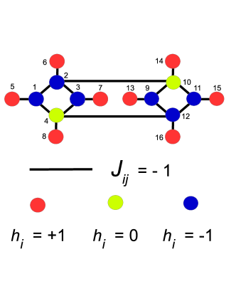
Figure 1: The 16-qubit instance. Qubits are denoted as circles, FM couplings as black lines. Colors correspond to biases applied to the qubits.

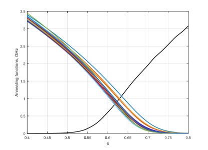
Figure 2: Annealing parameters ${\cal B}(s)$ (black line) and tunneling amplitudes $\Delta_{1}(s),...\Delta_{16}(s)$ (all other colors) plotted as functions of $s$.

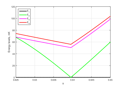
Figure 3: Four energy levels of the 16-qubit system as functions of the annealing parameter near the anticrossing of two lowest energy levels. Energies are counted from the energy $E_{1}$ of the ground state.

The two diabatic states with the lowest energies, $|GM\rangle$ and $|\Sigma\rangle$, are given by the expressions

$$|\rm GM\rangle=|\downarrow_{1}\downarrow_{2}\downarrow_{3}\downarrow_{4}\downarrow_{9}\downarrow_{10}\downarrow_{11}\downarrow_{12}\rangle\otimes$$

$$|\downarrow_{5}\downarrow_{6}\downarrow_{7}\downarrow_{8}\downarrow_{13}\downarrow_{14}\downarrow_{15}\downarrow_{16}\rangle,\;\,$$

$$|\Sigma\rangle=|\uparrow_{1}\uparrow_{2}\uparrow_{3}\uparrow_{4}\uparrow_{9}\uparrow_{10}\uparrow_{11}\uparrow_{12}\rangle\otimes$$

$$|\rightarrow_{5}\rightarrow_{6}\rightarrow_{7}\rightarrow_{8}\rightarrow_{13}\rightarrow_{14}\rightarrow_{15}\rightarrow_{16}\rangle.$$ (103)

Here we introduce the eigenstates $|\uparrow_{\alpha}\rangle$ and $|\downarrow_{\alpha}\rangle$ of the matrix $\sigma_{z}^{\alpha}$, and also their superposition $|\rightarrow_{\alpha}\rangle$,

$$\sigma_{z}^{\alpha}|\uparrow_{\alpha}\rangle=|\uparrow_{\alpha}\rangle,\quad\sigma_{z}^{\alpha}|\downarrow_{\alpha}\rangle=-|\downarrow_{\alpha}\rangle,$$

$$|\rightarrow_{\alpha}\rangle=\frac{1}{\sqrt{2}}(|\uparrow_{\alpha}\rangle+|\downarrow_{\alpha}\rangle).\quad\;$$

More details can be found in Ref. Dickson13 and in the supplementary information for that paper. It follows from Fig. 2c of Ref. Dickson13 that, before the anticrossing at $s<s^{*}$, the instantaneous eigenstates of the 16-qubit system coincide with the diabatic states: $|1\rangle=|\Sigma\rangle,$ $|2\rangle=|\rm GM\rangle.$ After the anticrossing point at $s>s^{*}$, we have the reverse situation, with $|1\rangle=|\rm GM\rangle$ and $|2\rangle=|\Sigma\rangle.$ Although the experimental results provided in Ref. Dickson13 were in accordance with the physical intuition given in the paper, no theoretical analysis was provided. This was due to the lack of an open quantum theory that takes into account both low-frequency and high-frequency noises. Here, we apply our approach to provide a theoretical explanation of the experimental results of Ref. Dickson13 .

The presence of a very small gap and the time-dependence of the system Hamiltonian, which becomes nonadiabatic near the minimum gap, make the problem instance in Fig. 1 difficult to analyze within one theoretical framework in all regions during the annealing. As such, some tricks are necessary to choose the proper basis as we discuss next.

VII.1 Rotation of the basis

The dissipative dynamics of the qubits coupled to a heat bath is described by the master equations (79). These equations are derived with the proviso that the rate $\Gamma_{nm}$ of the relaxation (88) between the states $|n\rangle$ and $|m\rangle$ is much less than the inverse time scale $\tau_{mn}^{-1}$ given by Eq. (85), so that: $\Gamma_{nm}\tau_{mn}\ll 1.$ For the system of 16 qubits under study the perturbation requirement breaks down at the anticrossing point as it is evident from Fig. 4a. Here we plot the energy gap, $E_{2}-E_{1}$, between two instantaneous eigenstates of the Hamiltonian $H_{S}$ (see dot-dashed blue line), and also the MRT line width, $W_{21}=a_{21}W$ (see continuous green line), as functions of the annealing parameter $s$. At $s=s^{*}$ both parameters, $E_{2}-E_{1}$ and $W_{21}$, become extremely small, leading to a diverging correlation time $\tau_{mn}$ (85). At the same time, $\Gamma_{12}$ becomes very large due to the contribution from $\tilde{T}_{21}$. Both of these break the applicability condition (84) in the instantaneous energy basis. Moreover, the time dependence of the Hamiltonian can create nonzero off-diagonal elements of the density matrix near the minimum gap due to nonadiabatic transitions. These terms do not decay quickly as required by our theory. As we shall see, all these issues can be resolved by rotating the basis. This is equivalent to the introduction of the pointer basis as described in Refs. Boixo16 ; Boixo14 ; Zurek03 .

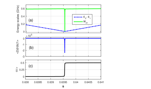
Figure 4: (a) The energy scales $E_{2}-E_{1}$ and the line width $W_{21}=Wa_{21}$ calculated in the instantaneous basis of qubit states. These variables are shown as functions of the annealing parameter $s$ near the anticrossing point. According to (85), the scales $E_{2}-E_{1}$ and $W_{21}$ determine the inverse correlation time $\tau_{21}^{-1}$ of the bath. (b) The $s$-dependence of the matrix element $\langle 2|\frac{d}{ds}|1\rangle$ calculated with Eq. (69). This matrix element is a part of the renormalized tunneling coefficient $\bar{T}_{mn}$ (81) and, thus, of the rate $\Gamma_{21}$ (IV.1). (c) The optimal rotation angle $\Theta/\pi$ obtained as a solution of Eq. (106).

We rotate the two anticrossing states as:

$$|1^{\prime}\rangle = \cos\Theta\;|1\rangle+\sin\Theta\;|2\rangle,$$

$$|2^{\prime}\rangle = -\sin\Theta\;|1\rangle+\cos\Theta\;|2\rangle.$$ (104)

The rotation angle $\Theta$ can depend on the annealing parameter $s$ and therefore on time $t$. For real eigenstates $|1\rangle$ and $|2\rangle$ it follows that

$$\langle 2^{\prime}|\frac{d}{ds}|1^{\prime}\rangle=\langle 2|\frac{d}{ds}|1\rangle+\frac{d\Theta}{ds}.$$

We choose the rotation angle $\Theta(s)$ such that in the rotated basis

$$\langle 2^{\prime}|\frac{d}{ds}|1^{\prime}\rangle=0.$$ (105)

This means that the $s$-dependence of the angle $\Theta$ is determined by

$$\frac{d\Theta}{ds}=\frac{\langle 2|\frac{dH_{S}}{ds}|1\rangle}{E_{2}-E_{1}}.$$ (106)

Notice that (105) assures minimum quantum transition between the two states $|1^{\prime}\rangle$ and $|2^{\prime}\rangle$ near the anticrossing and therefore minimum generation of off-diagonal elements of the density matrix. As we show in Appendix F, it also resolves all issues with the applicability condition (84) discussed above.

A solution of Eq. (106) is shown in Fig. 4c. In the beginning of annealing $\Theta\simeq 0$, so that the rotated basis coincides with the instantaneous basis. Near the anticrossing point, at $s=s^{*}$, the angle $\Theta$ rapidly switches to $\pi/2$. We notice that, with the condition (105), the renormalized matrix element $\tilde{T}_{2^{\prime}1^{\prime}}$ (68) is

$$\tilde{T}_{2^{\prime}1^{\prime}}=\langle 2^{\prime}|H_{S}|1^{\prime}\rangle=\frac{E_{2}-E_{1}}{2}\,\sin 2\Theta.$$ (107)

This is zero before ($\Theta=0$) and after ($\Theta=\pi/2$) the anticrossing due to the sine function and is very small at the anticrossing due to the small gap ($E_{2}-E_{1}\approx 0$). This means that $\tilde{T}_{2^{\prime}1^{\prime}}$ does not contribute to the rate $\Gamma_{1^{\prime}2^{\prime}}$ keeping it small, within the applicability range of our model. For this example we rotate only the two lowest-energy states that have an anticrossing. However, the rotation can be applied to anticrossing excited states as well, if necessary.

VII.2 Thermal enhancement of the success probability

The goal of annealing is to reach the ground state at the end of the evolution. It follows from Fig. 2c of Ref. Dickson13 that at the end of annealing, at $t=t_{f}$, the ground state of the 16-qubit system coincides with the state $|\rm GM\rangle$ shown in Eq. (VII). We therefore define the success probability as the probability $P_{\rm GM}$ to observe the system in $|\rm GM\rangle$ at $t=t_{f}$. Figure 3 of Ref.Dickson13 demonstrates the temperature dependence of $P_{\rm GM}$. It is clear from this figure that, at sufficiently fast annealing ($t_{f}\leq 100$ ms), $P_{\rm GM}$ grows with increasing temperature from 20 to 40 mK and decreases after. Our goal is to reproduce this non-monotonic behavior with our open quantum model. Notice that we do not aim to precisely fit the experimental data to the results of our model.

We solve numerically the master equations (79) with the relaxation rates given by the convolution formula (88) written in the rotated basis (VII.1). We perform simulation for the total anneal time $t_{f}$ between 0.04 to 4 ms. An example of $P_{\rm GM}$ as a function of time is shown in Fig. 9b in Appendix F. Fig. 5 plots the success probability, $P_{\rm GM}(t_{f}),$ as a function of temperature $T$ for different speeds of annealing characterized by the anneal time $t_{f}$. In the theoretical calculations we assume that $\eta=0.1$ and $W=20$ mK.

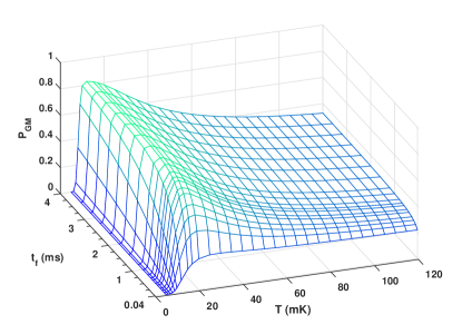
Figure 5: End-of-annealing probability to be in the $|\rm GM\rangle$ state, $P_{\rm GM}$, as a function of temperature $T$ and the anneal time $t_{f}$ at $\eta=0.1$ and $W=20$ mK.

Figure 5 reproduces the results shown in Fig. 3 of Ref.Dickson13 , including the enhancement $P_{\rm GM}$ at low temperatures and its reduction at $T\geq 40$ mK. As mentioned in Ref. Dickson13 , this decrease may be related to the excitement of the high-energy levels separated from the two lowest states by a gap of order 40 mK (see the spectrum in Fig. 3).

VIII Conclusions

In this paper, we have derived a set of master equations describing a dissipative evolution of an open quantum system interacting with a complex environment. The environment has low-frequency and high-frequency components, as in the case of realistic qubits affected by the hybrid bath, which includes $1/f$ and Ohmic noise. A part of the system-bath interaction is treated in a nonperturbative way. This treatment allows us to combine the Bloch-Redfield and Marcus approaches to the theory of open quantum systems and obtain the relaxation rates, which are well-suited for the description of dissipative dynamics of many-qubit quantum objects, such as quantum annealers. The relaxation rates are expressed in the convenient convolution form clearly showing the interplay between the low- and high-frequency noise. The main results of the paper are given by the master equations (79) with the relaxation rates (88). As an illustration, we apply the theory to the 16-qubit quantum annealer investigated in Ref. Dickson13 . The instance studied there features an extremely small gap between the ground and first excited states. With the proper rotation of the basis, we have solved the master equations and theoretically confirmed the main experimental findings of Ref. Dickson13 . The results of the paper may be useful for understanding a dissipative evolution of various systems, from chromophores in quantum biology Yang02 ; Ghosh11 ; Lambert13 to qubits in real-world quantum processors Gibney17 ; Mohseni17 .

Appendix A Notations

In this appendix we assemble notations used throughout the paper, so that the main part of the paper becomes easier to follow. In a chosen basis $\{|n\rangle\}$ the matrix elements of the system Hamiltonian $H_{S}$ (18) and those of the Pauli matrix $\sigma_{z}^{\alpha}$ of the $\alpha$-qubit are denoted as

$$E_{n}=\langle n|H_{S}|n\rangle,\quad T_{mn}=\langle m|H_{S}|n\rangle,$$

$$\sigma^{\alpha}_{n}=\langle n|\sigma_{z}^{\alpha}|n\rangle,\quad\sigma^{\alpha}_{mn}=\langle m|\sigma_{z}^{\alpha}|n\rangle.$$ (108)

For combinations of the matrix elements we introduce the following notations:

$$a_{mn}=\sum_{\alpha}(\sigma_{m}^{\alpha}-\sigma_{n}^{\alpha})^{2},\;b_{mn}=\sum_{\alpha}|\sigma^{\alpha}_{mn}|^{2},\hskip 21.33955pt$$ (109)

$$c_{mn}=\sum_{\alpha}\sigma^{\alpha}_{mn}(\sigma_{m}^{\alpha}-\sigma_{n}^{\alpha}),\;d_{mn}=\sum_{\alpha}\sigma^{\alpha}_{mn}(\sigma_{m}^{\alpha}+\sigma_{n}^{\alpha}).$$

The parameters of the bath are defined as

$$\varepsilon_{L}=\int\frac{d\omega}{2\pi}\frac{S_{L}(\omega)}{\omega},\quad\varepsilon_{H}=\frac{\eta\omega_{c}}{2\pi},\quad\varepsilon=\varepsilon_{L}+\varepsilon_{H},$$

$$W^{2}=\int\frac{d\omega}{2\pi}S_{L}(\omega)=2\,\varepsilon_{L}T,\hskip 42.67912pt$$ (110)

with $\eta$ and $\omega_{c}$ defined in Sec. III-E. We also introduce

$$\varepsilon_{mn}=a_{mn}\varepsilon_{L},\quad W_{mn}^{2}=a_{mn}W^{2},$$

$$\eta_{mn}=a_{mn}\eta,\quad\gamma_{mn}=\frac{1}{2}\,\eta_{mn}T.$$ (111)

For a time-dependent basis $|n(t)\rangle$, we write the following functions of time:

$$\omega_{mn}(t)=E_{m}(t)-E_{n}(t),$$

$$\phi_{mn}(t)=\int_{0}^{t}d\tau\,\omega_{mn}(\tau),$$

$$\tilde{T}_{mn}=T_{mn}-i\,\langle m|\dot{n}\rangle,$$

$$\bar{T}_{mn}=T_{mn}-i\,\langle m|\dot{n}\rangle-d_{mn}\,\varepsilon.$$ (112)

The coefficients $A_{mn},B_{mn}$ used in Eqs. (88) and (89) are defined as

$$A_{mn}=\bar{T}_{mn}-\omega_{mn}\,\frac{c_{mn}}{a_{mn}},$$

$$B_{mn}=\frac{a_{mn}b_{mn}-|c_{mn}|^{2}}{a_{mn}^{2}}=$$

$$\frac{1}{2a_{mn}^{2}}\;\sum_{\alpha\beta}|(\sigma_{m}^{\alpha}-\sigma_{n}^{\alpha})\,\sigma_{mn}^{\beta}-(\sigma_{m}^{\beta}-\sigma_{n}^{\beta})\,\sigma_{mn}^{\alpha}|^{2}.$$ (113)

Appendix B High-frequency dissipative functions

For the Ohmic high-frequency bath characterized by the spectrum (44) the dissipative functions $f_{H},g_{H}$ and a correlator $K_{H}=\ddot{f}_{H}$ are given by the formulas

$$f_{H}(t)=\frac{\eta}{2\pi}\,\ln\left[(1+i\omega_{c}t)\,\frac{\sinh(\pi Tt)}{\pi Tt}\right],\;\;$$ (114)

$$g_{H}(t)=\frac{\eta}{2\pi}\,\frac{\omega_{c}}{1+i\omega_{c}t}-i\frac{\eta T}{2}\,\left[\coth(\pi Tt)-\frac{1}{\pi Tt}\right],$$

$$K_{H}(t)=\frac{\eta}{2\pi}\,\left\{\left(\frac{\omega_{c}}{1+i\omega_{c}t}\right)^{2}-\left[\frac{\pi T}{\sinh(\pi Tt)}\right]^{2}+\frac{1}{t^{2}}\right\},$$

provided that the cutting frequency $\omega_{c}$ is much higher than the temperature, $\hbar\omega_{c}\gg k_{B}T.$ We notice that at large times, $t\gg\frac{\hbar}{\pi k_{B}T}$, all the three functions vanish. In Eq. (44) we introduce $\eta$ as a small dimensionless coupling constant Leggett87 , and $\omega_{c}$ as a large cutting frequency of the high-frequency noise. For the Ohmic bath, the spectral density $\chi_{H}^{\prime\prime}(\omega)$ is defined as

$$\chi_{H}^{\prime\prime}(\omega)=\frac{\eta\omega}{2}\,e^{-|\omega|/\omega_{c}}.$$ (115)

We assume independent noise sources coupled to every qubit, each described by the above-mentioned formulas with identical parameters.

Appendix C Correlator $\tilde{K}_{mn}^{m^{\prime}n^{\prime}}(t,t^{\prime})$

Here we calculate the correlator (70) of the nondiagonal bath variables with indexes $m\neq n$ and $m^{\prime}\neq n^{\prime}$. In this case, the bath operators are defined by Eq. (64), and the correlator $\tilde{K}_{mn}^{m^{\prime}n^{\prime}}(t,t^{\prime})$ is given by the formula

$$\tilde{K}_{mn}^{m^{\prime}n^{\prime}}(t,t^{\prime})=e^{i\phi_{mn}(t)}e^{i\phi_{m^{\prime}n^{\prime}}(t^{\prime})}\times$$

$$\langle{\cal S}^{\dagger}_{m}(t)[Q_{mn}(t)-\tilde{T}_{mn}(t)]{\cal S}_{n}(t)\times$$

$${\cal S}^{\dagger}_{m^{\prime}}(t^{\prime})[Q_{m^{\prime}n^{\prime}}(t^{\prime})-\tilde{T}_{m^{\prime}n^{\prime}}(t^{\prime})]{\cal S}_{n^{\prime}}(t^{\prime})\rangle.$$ (116)

This correlator can be represented as a sum of four components:

$$\tilde{K}_{mn}^{m^{\prime}n^{\prime}}(t,t^{\prime})=e^{i\int_{0}^{t}d\tau\,\omega_{mn}(\tau)+i\int_{0}^{t^{\prime}}d\tau\,\omega_{m^{\prime}n^{\prime}}(\tau)}\times$$

$$\{(i)+(ii)+(iii)+(iv)\},\hskip 28.45274pt$$ (117)

with

$$(i)=\tilde{T}_{mn}\,\tilde{T}_{m^{\prime}n^{\prime}}\;F_{mn}^{m^{\prime}n^{\prime}}(t,t^{\prime}),$$ (118)

$$(ii)=-\tilde{T}_{mn}\langle{\cal S}_{m}^{\dagger}(t){\cal S}_{n}(t){\cal S}_{m^{\prime}}^{\dagger}(t^{\prime})Q_{m^{\prime}n^{\prime}}(t^{\prime}){\cal S}_{n^{\prime}}(t^{\prime})\rangle,$$

$$(iii)=-\tilde{T}_{m^{\prime}n^{\prime}}\langle{\cal S}_{m}^{\dagger}(t)Q_{mn}(t){\cal S}_{n}(t){\cal S}_{m^{\prime}}^{\dagger}(t^{\prime}){\cal S}_{n^{\prime}}(t^{\prime})\rangle,$$

$$(iv)=\langle{\cal S}_{m}^{\dagger}(t)Q_{mn}(t){\cal S}_{n}(t){\cal S}_{m^{\prime}}^{\dagger}(t^{\prime})Q_{m^{\prime}n^{\prime}}(t^{\prime}){\cal S}_{n^{\prime}}(t^{\prime})\rangle,$$

where

$$F_{mn}^{m^{\prime}n^{\prime}}(t,t^{\prime})=\langle{\cal S}_{m}^{\dagger}(t){\cal S}_{n}(t){\cal S}_{m^{\prime}}^{\dagger}(t^{\prime}){\cal S}_{n^{\prime}}(t^{\prime})\rangle.$$ (119)

The bath variable $Q_{mn}$ is defined in (III.6), and ${\cal S}_{n}$ is the $S$-matrix of the bath given by Eq. (57).

C.1 Term $(i)$ and the functional $F_{mn}^{m^{\prime}n^{\prime}}$

To calculate the functional $F_{mn}^{m^{\prime}n^{\prime}}(t,t^{\prime})$ (119) we consider a more complicated term

$${\cal F}_{mn}^{m^{\prime}n^{\prime}}(t,\tau;t^{\prime},\tau^{\prime})=$$

$$\langle{\cal S}_{m}^{\dagger}(t,\tau){\cal S}_{n}(t,\tau){\cal S}_{m^{\prime}}^{\dagger}(t^{\prime},\tau^{\prime}){\cal S}_{n^{\prime}}(t^{\prime},\tau^{\prime})\rangle,$$ (120)

where the modified $S$-matrix of the bath, ${\cal S}_{n}(t,\tau),$ is defined by Eq. (61). We notice that

$$F_{mn}^{m^{\prime}n^{\prime}}(t,t^{\prime})={\cal F}_{mn}^{m^{\prime}n^{\prime}}(t,t;t^{\prime},t^{\prime}).$$ (121)

The functional ${\cal F}_{mn}^{m^{\prime}n^{\prime}}(t,\tau;t^{\prime},\tau^{\prime})$ obeys two differential equations:

$$\frac{d}{d\tau}\,{\cal F}_{mn}^{m^{\prime}n^{\prime}}(t,\tau;t^{\prime},\tau^{\prime})=i\sum_{\alpha}\tilde{\sigma}_{nm}^{\alpha}(t)\times$$

$$\langle{\cal S}_{m}^{\dagger}(t,\tau)Q_{\alpha}(\tau){\cal S}_{n}(t,\tau){\cal S}_{m^{\prime}}^{\dagger}(t^{\prime},\tau^{\prime}){\cal S}_{n^{\prime}}(t^{\prime},\tau^{\prime})\rangle,$$

$$\frac{d}{d\tau^{\prime}}\,{\cal F}_{mn}^{m^{\prime}n^{\prime}}(t,\tau;t^{\prime},\tau^{\prime})=i\sum_{\alpha}\tilde{\sigma}_{n^{\prime}m^{\prime}}^{\alpha}(t^{\prime})\times$$

$$\langle{\cal S}_{m}^{\dagger}(t,\tau){\cal S}_{n}(t,\tau){\cal S}_{m^{\prime}}^{\dagger}(t^{\prime},\tau^{\prime})Q_{\alpha}(\tau^{\prime}){\cal S}_{n^{\prime}}(t^{\prime},\tau^{\prime})\rangle,$$ (122)

where we introduce the notation $\tilde{\sigma}_{nm}^{\alpha}(t)=\sigma_{n}^{\alpha}(t)-\sigma_{m}^{\alpha}(t).$ With the Wick theorem BSH , we have to take all possible pairings of the Gaussian operators $Q_{\alpha}(\tau)$ and $Q_{\alpha}(\tau^{\prime})$ in Eq. (C.1) with other operators. As a result, we obtain

$$\frac{d}{d\tau}\,\ln{\cal F}_{mn}^{m^{\prime}n^{\prime}}(t,\tau;t^{\prime},\tau^{\prime})=\sum_{\alpha}\tilde{\sigma}_{mn}^{\alpha}(t)\times$$

$$\int_{0}^{\tau}d\tau_{1}\left[\,\sigma_{n}^{\alpha}(t)\,K_{\alpha}(\tau,\tau_{1})-\sigma_{m}^{\alpha}(t)\,K_{\alpha}(\tau_{1},\tau)\,\right]-$$

$$\sum_{\alpha}\tilde{\sigma}_{mn}^{\alpha}(t)\,\tilde{\sigma}_{m^{\prime}n^{\prime}}^{\alpha}(t^{\prime})\,\int_{0}^{\tau^{\prime}}d\tau_{1}\,\,K_{\alpha}(\tau,\tau_{1}),$$

$$\frac{d}{d\tau^{\prime}}\,\ln{\cal F}_{mn}^{m^{\prime}n^{\prime}}(t,\tau;t^{\prime},\tau^{\prime})=\sum_{\alpha}\tilde{\sigma}_{m^{\prime}n^{\prime}}^{\alpha}(t^{\prime})\times$$

$$\int_{0}^{\tau^{\prime}}d\tau_{1}\left[\,\sigma_{n^{\prime}}^{\alpha}(t^{\prime})\,K_{\alpha}(\tau^{\prime},\tau_{1})-\sigma_{m^{\prime}}^{\alpha}(t^{\prime})\,K_{\alpha}(\tau_{1},\tau^{\prime})\,\right]-$$

$$\sum_{\alpha}\tilde{\sigma}_{mn}^{\alpha}(t)\,\tilde{\sigma}_{m^{\prime}n^{\prime}}^{\alpha}(t^{\prime})\int_{0}^{\tau}d\tau_{1}\,\,K_{\alpha}(\tau_{1},\tau^{\prime}).$$ (123)

The solution of these two equations is given by the expression

$$\ln{\cal F}_{mn}^{m^{\prime}n^{\prime}}(t,\tau;t^{\prime},\tau^{\prime})=$$

$$-\sum_{\alpha}\tilde{\sigma}_{mn}^{\alpha}(t)\,\tilde{\sigma}_{m^{\prime}n^{\prime}}^{\alpha}(t^{\prime})\int_{0}^{\tau}d\tau_{1}\int_{0}^{\tau^{\prime}}d\tau_{2}\,K_{\alpha}(\tau_{1},\tau_{2})+$$

$$\sum_{\alpha}\tilde{\sigma}_{mn}^{\alpha}(t)\,\int_{0}^{\tau}d\tau_{1}\int_{0}^{\tau_{1}}d\tau_{2}\times$$

$$\left[\sigma_{n}^{\alpha}(t)\,K_{\alpha}(\tau_{1},\tau_{2})-\sigma_{m}^{\alpha}(t)\,K_{\alpha}(\tau_{2},\tau_{1})\,\right]+$$

$$\sum_{\alpha}\tilde{\sigma}_{m^{\prime}n^{\prime}}^{\alpha}(t^{\prime})\,\int_{0}^{\tau^{\prime}}d\tau_{1}\int_{0}^{\tau_{1}}d\tau_{2}\times$$

$$\left[\sigma_{n^{\prime}}^{\alpha}(t^{\prime})\,K_{\alpha}(\tau_{1},\tau_{2})-\sigma_{m^{\prime}}^{\alpha}(t^{\prime})\,K_{\alpha}(\tau_{2},\tau_{1})\,\right].$$ (124)

It follows from Eq. (121) that the functional $F_{mn}^{m^{\prime}n^{\prime}}(t,t^{\prime})$ of the Gaussian bath is described by the formula

$$F_{mn}^{m^{\prime}n^{\prime}}(t,t^{\prime})=$$

$$\exp\left\{-\sum_{\alpha}(\sigma_{m}^{\alpha}-\sigma_{n}^{\alpha})(t)\,(\sigma_{m^{\prime}}^{\alpha}-\sigma_{n^{\prime}}^{\alpha})(t^{\prime})\times\right.$$

$$\left.\int_{0}^{t}d\tau_{1}\int_{0}^{t^{\prime}}d\tau_{2}\,K_{\alpha}(\tau_{1},\tau_{2})+\right.$$

$$\left.\sum_{\alpha}(\sigma_{m}^{\alpha}-\sigma_{n}^{\alpha})(t)\,\int_{0}^{t}d\tau_{1}\int_{0}^{\tau_{1}}d\tau_{2}\times\right.$$

$$\left.\left[\sigma_{n}^{\alpha}(t)\,K_{\alpha}(\tau_{1},\tau_{2})-\sigma_{m}^{\alpha}(t)\,K_{\alpha}(\tau_{2},\tau_{1})\,\right]+\right.$$

$$\left.\sum_{\alpha}(\sigma_{m^{\prime}}^{\alpha}-\sigma_{n^{\prime}}^{\alpha})(t^{\prime})\,\int_{0}^{t^{\prime}}d\tau_{1}\int_{0}^{\tau_{1}}d\tau_{2}\times\right.$$

$$\left.\left[\sigma_{n^{\prime}}^{\alpha}(t^{\prime})\,K_{\alpha}(\tau_{1},\tau_{2})-\sigma_{m^{\prime}}^{\alpha}(t^{\prime})\,K_{\alpha}(\tau_{2},\tau_{1})\,\right]\right\}.$$ (125)

Here $K_{\alpha}(t,t^{\prime})$ is the correlation function (34) of the free bath.

C.2 Terms $(ii)$ and $(iii)$

Using the Wick theorem BSH , we find that the terms $(ii)$ and $(iii)$ are proportional to the correlators

$$\langle{\cal S}_{m}^{\dagger}(t){\cal S}_{n}(t){\cal S}_{m^{\prime}}^{\dagger}(t^{\prime})Q_{m^{\prime}n^{\prime}}(t^{\prime}){\cal S}_{n^{\prime}}(t^{\prime})\rangle=$$

$$i\,\sum_{\alpha}\sigma_{m^{\prime}n^{\prime}}^{\alpha}(t^{\prime})\,F_{mn}^{m^{\prime}n^{\prime}}(t,t^{\prime})\times$$

$$\left\{(\sigma_{n}^{\alpha}-\sigma_{m}^{\alpha})(t)\int_{0}^{t}dt_{1}K_{\alpha}(t_{1},t^{\prime})+\right.$$

$$\left.\int_{0}^{t^{\prime}}dt_{1}[\,\sigma_{n^{\prime}}^{\alpha}(t^{\prime})\,K_{\alpha}(t^{\prime},t_{1})-\sigma_{m^{\prime}}^{\alpha}(t^{\prime})\,K_{\alpha}(t_{1},t^{\prime})\,]\right\},$$

$$\langle{\cal S}_{m}^{\dagger}(t)Q_{mn}(t){\cal S}_{n}(t){\cal S}_{m^{\prime}}^{\dagger}(t^{\prime}){\cal S}_{n^{\prime}}(t^{\prime})\rangle=$$

$$i\,\sum_{\alpha}\sigma_{mn}^{\alpha}(t)\,F_{mn}^{m^{\prime}n^{\prime}}(t,t^{\prime})\times$$

$$\left\{(\sigma_{n^{\prime}}^{\alpha}-\sigma_{m^{\prime}}^{\alpha})(t^{\prime})\int_{0}^{t^{\prime}}dt_{1}K_{\alpha}(t,t_{1})+\right.$$

$$\left.\int_{0}^{t}dt_{1}[\,\sigma_{n}^{\alpha}(t)\,K_{\alpha}(t,t_{1})-\sigma_{m}^{\alpha}(t)\,K_{\alpha}(t_{1},t)\,]\right\}.$$ (126)

C.3 Term $(iv)$ and the total correlator

The last term in Eq. (118) can be written as

$$\langle{\cal S}_{m}^{\dagger}(t)Q_{mn}(t){\cal S}_{n}(t){\cal S}_{m^{\prime}}^{\dagger}(t^{\prime})Q_{m^{\prime}n^{\prime}}(t^{\prime}){\cal S}_{n^{\prime}}(t^{\prime})\rangle=$$

$$\sum_{\alpha}\sigma_{mn}^{\alpha}(t)\,\sigma_{m^{\prime}n^{\prime}}^{\alpha}(t^{\prime})\,K_{\alpha}(t,t^{\prime})\,F_{mn}^{m^{\prime}n^{\prime}}(t,t^{\prime})+$$

$$i^{2}\sum_{\alpha\alpha^{\prime}}\sigma_{mn}^{\alpha}(t)\,\sigma_{m^{\prime}n^{\prime}}^{\alpha^{\prime}}(t^{\prime})\,F_{mn}^{m^{\prime}n^{\prime}}(t,t^{\prime})\times$$

$$\left\{\int_{0}^{t}dt_{1}[\,\sigma_{n}^{\alpha}(t)\,K_{\alpha}(t,t_{1})-\sigma_{m}^{\alpha}(t)\,K_{\alpha}(t_{1},t)\,]+\right.$$

$$\left.(\sigma_{n^{\prime}}^{\alpha}-\sigma_{m^{\prime}}^{\alpha})(t^{\prime})\int_{0}^{t^{\prime}}dt_{1}K_{\alpha}(t,t_{1})\right\}\times$$

$$\left\{\int_{0}^{t^{\prime}}dt_{1}[\,\sigma_{n^{\prime}}^{\alpha^{\prime}}(t^{\prime})\,K_{\alpha^{\prime}}(t^{\prime},t_{1})-\sigma_{m^{\prime}}^{\alpha^{\prime}}(t^{\prime})\,K_{\alpha^{\prime}}(t_{1},t^{\prime})\,]+\right.$$

$$\left.(\sigma_{n}^{\alpha^{\prime}}-\sigma_{m}^{\alpha^{\prime}})(t)\int_{0}^{t}dt_{1}K_{\alpha^{\prime}}(t_{1},t^{\prime}))\right\}.\hskip 28.45274pt$$ (127)

The correlation function (C) of the operators $\tilde{Q}_{mn}(t)$ and $\tilde{Q}_{m^{\prime}n^{\prime}}(t^{\prime})$ has the form

$$\tilde{K}_{mn}^{m^{\prime}n^{\prime}}(t,t^{\prime})=e^{i\phi_{mn}(t)}e^{i\phi_{m^{\prime}n^{\prime}}(t^{\prime})}\times\hskip 14.22636pt$$ (128)

$$\{{\cal K}_{mn}^{m^{\prime}n^{\prime}}(t,t^{\prime})+{\cal U}_{mn}^{m^{\prime}n^{\prime}}(t,t^{\prime})\,{\cal V}_{m^{\prime}n^{\prime}}^{mn}(t^{\prime},t)\}\,F_{mn}^{m^{\prime}n^{\prime}}(t,t^{\prime}),$$

where

$${\cal K}_{mn}^{m^{\prime}n^{\prime}}(t,t^{\prime})=\sum_{\alpha}\sigma_{mn}^{\alpha}(t)\,\sigma_{m^{\prime}n^{\prime}}^{\alpha}(t^{\prime})\,K_{\alpha}(t,t^{\prime}),\hskip 14.22636pt$$ (129)

$${\cal U}_{mn}^{m^{\prime}n^{\prime}}(t,t^{\prime})=\tilde{T}_{mn}(t)-$$

$$i\sum_{\alpha}\sigma_{mn}^{\alpha}(t)\left\{(\sigma_{n^{\prime}}^{\alpha}-\sigma_{m^{\prime}}^{\alpha})(t^{\prime})\int_{0}^{t^{\prime}}dt_{1}K_{\alpha}(t,t_{1})+\right.$$

$$\left.\int_{0}^{t}dt_{1}[\,\sigma_{n}^{\alpha}(t)\,K_{\alpha}(t,t_{1})-\sigma_{m}^{\alpha}(t)\,K_{\alpha}(t_{1},t)\,]\right\},$$

$${\cal V}^{mn}_{m^{\prime}n^{\prime}}(t^{\prime},t)=\tilde{T}_{m^{\prime}n^{\prime}}(t^{\prime})-$$

$$i\sum_{\alpha}\sigma_{m^{\prime}n^{\prime}}^{\alpha}(t^{\prime})\left\{(\sigma_{n}^{\alpha}-\sigma_{m}^{\alpha})(t)\int_{0}^{t}dt_{1}K_{\alpha}(t_{1},t^{\prime})+\right.$$

$$\left.\int_{0}^{t^{\prime}}dt_{1}[\,\sigma_{n^{\prime}}^{\alpha}(t^{\prime})\,K_{\alpha}(t^{\prime},t_{1})-\sigma_{m^{\prime}}^{\alpha}(t^{\prime})\,K_{\alpha}(t_{1},t^{\prime})\,]\right\}.$$

We notice that

$$\left[F_{mn}^{m^{\prime}n^{\prime}}(t,t^{\prime})\right]^{\dagger}=F_{n^{\prime}m^{\prime}}^{nm}(t^{\prime},t),$$

$$\left[\,{\cal K}_{mn}^{m^{\prime}n^{\prime}}(t,t^{\prime})\,\right]^{\dagger}={\cal K}_{nm}^{n^{\prime}m^{\prime}}(t^{\prime},t),$$

$$\left[\,{\cal U}_{mn}^{m^{\prime}n^{\prime}}(t,t^{\prime})\,\right]^{\dagger}={\cal V}_{nm}^{n^{\prime}m^{\prime}}(t,t^{\prime}),$$

$$\left[\,{\cal V}^{mn}_{m^{\prime}n^{\prime}}(t^{\prime},t)\,\right]^{\dagger}={\cal U}^{nm}_{n^{\prime}m^{\prime}}(t^{\prime},t).$$ (130)

C.4 Correlators and dissipative functions

The correlation function of the bath (128) and the functional (C.1) can be rewritten in terms of the dissipative functions defined by Eq. (III.4). Taking into account integrals, such as

$$\int_{0}^{t}dt_{1}\int_{0}^{t^{\prime}}dt_{2}\,K_{\alpha}(t_{1},t_{2})=f_{\alpha}(t)+f_{\alpha}^{*}(t^{\prime})-f_{\alpha}(t-t^{\prime}),$$

$$\int_{0}^{t}dt_{1}\int_{0}^{t_{1}}dt_{2}K_{\alpha}(t_{1},t_{2})=-i\,\varepsilon_{\alpha}\,t+f_{\alpha}(t),\hskip 28.45274pt$$

we find that

$$\ln F_{mn}^{m^{\prime}n^{\prime}}(t,t^{\prime})=\sum_{\alpha}(\sigma_{m}^{\alpha}-\sigma_{n}^{\alpha})(\sigma_{m^{\prime}}^{\alpha}-\sigma_{n^{\prime}}^{\alpha})\,f_{\alpha}(t-t^{\prime})-$$

$$i\sum_{\alpha}\varepsilon_{\alpha}[(\sigma_{m}^{\alpha})^{2}-(\sigma_{n}^{\alpha})^{2}]\,t-i\sum_{\alpha}\varepsilon_{\alpha}[(\sigma_{m^{\prime}}^{\alpha})^{2}-(\sigma_{n^{\prime}}^{\alpha})^{2}]\,t^{\prime}+$$

$$\sum_{\alpha}(\sigma_{m}^{\alpha}-\sigma_{n}^{\alpha})(\sigma_{n}^{\alpha}-\sigma_{m^{\prime}}^{\alpha}+\sigma_{n^{\prime}}^{\alpha})f_{\alpha}(t)-\hskip 28.45274pt$$

$$\sum_{\alpha}(\sigma_{m^{\prime}}^{\alpha}-\sigma_{n^{\prime}}^{\alpha})(\sigma_{m^{\prime}}^{\alpha}+\sigma_{m}^{\alpha}-\sigma_{n}^{\alpha})f_{\alpha}^{*}(t^{\prime})\hskip 35.56593pt$$ (131)

$$+\sum_{\alpha}(\sigma_{m^{\prime}}^{\alpha}-\sigma_{n^{\prime}}^{\alpha})\sigma_{n^{\prime}}^{\alpha}f_{\alpha}(t^{\prime})-\sum_{\alpha}(\sigma_{m}^{\alpha}-\sigma_{n}^{\alpha})\sigma_{m}^{\alpha}f_{\alpha}^{*}(t).$$

Here the matrix elements $\sigma_{m}^{\alpha}$ and $\sigma_{n}^{\alpha}$ are taken at time $t$, whereas the elements $\sigma_{m^{\prime}}^{\alpha}$ and $\sigma_{n^{\prime}}^{\alpha}$ depend on the time $t^{\prime}$. The total reorganization energy $\varepsilon_{\alpha}$ is defined by Eq. (38).

With Eq. (C.4) we can calculate the correlator $\langle{\cal S}_{m}^{\dagger}(t){\cal S}_{n}(t)\rangle$. It follows from Eqs. (57) and (119) that this correlator is determined by Eqs. (121) and (C.1) where we have to put $t^{\prime}=0$:

$$\langle{\cal S}^{\dagger}_{m}(t){\cal S}_{n}(t)\rangle=F_{mn}^{m^{\prime}n^{\prime}}(t,t^{\prime}=0)=\;\;$$

$$\exp\left[-\sum_{\alpha}(\sigma_{m}^{\alpha}-\sigma_{n}^{\alpha})^{2}\,f^{\prime}_{\alpha}(t)\right]\,e^{i\vartheta_{mn}(t)},$$ (132)

with the phase

$$\vartheta_{mn}(t)=\sum_{\alpha}\,[(\sigma_{m}^{\alpha})^{2}-(\sigma_{n}^{\alpha})^{2}]\;[f_{\alpha}^{\prime\prime}(t)-\varepsilon_{\alpha}t].$$ (133)

Taking into account Eqs. (43) and (114) we find that

$$\langle{\cal S}^{\dagger}_{m}(t){\cal S}_{n}(t)\rangle=e^{-\frac{1}{2}W^{2}_{mn}t^{2}}\,e^{i\vartheta_{mn}(t)}\times$$

$$\left[\sqrt{1+\omega_{c}^{2}t^{2}}\;\frac{\sinh(\pi Tt)}{\pi Tt}\right]^{-\frac{\eta_{mn}}{2\pi}}.$$ (134)

Low-frequency, $W_{mn}^{2}=a_{mn}W^{2}$, and high-frequency, $\eta_{mn}=a_{mn}\eta$, parameters are proportional to the Hamming distance $a_{mn}$ between states $|m\rangle$ and $|n\rangle$ (49). At $a_{mn}\neq 0$ the function $\langle{\cal S}^{\dagger}_{m}{\cal S}_{n}\rangle$ rapidly decays within the time scale of $1/W_{mn}$. The average value of the operator (64) also does not survive during the annealing process since

$$\langle\tilde{Q}_{mn}(t)\rangle\sim e^{i\omega_{mn}t}\,\langle{\cal S}^{\dagger}_{m}(t){\cal S}_{n}(t)\rangle\sim 0.$$ (135)

C.5 Selection rules

The real part of the exponent (C.4) has the form

$$\Re\,\{\,\ln F_{mn}^{m^{\prime}n^{\prime}}(t,t^{\prime})\,\}=\hskip 28.45274pt$$ (136)

$$\sum_{\alpha}(\sigma_{m}^{\alpha}-\sigma_{n}^{\alpha})(\sigma_{m^{\prime}}^{\alpha}-\sigma_{n^{\prime}}^{\alpha})\,f_{\alpha}^{\prime}(t-t^{\prime})\hskip 28.45274pt$$

$$-\sum_{\alpha}[(\sigma_{m}^{\alpha}-\sigma_{n}^{\alpha})^{2}-(\sigma_{m^{\prime}}^{\alpha}-\sigma_{n^{\prime}}^{\alpha})^{2}]\,\frac{f_{\alpha}^{\prime}(t)-f_{\alpha}^{\prime}(t^{\prime})}{2}$$

$$-\sum_{\alpha}(\sigma_{m}^{\alpha}-\sigma_{n}^{\alpha}+\sigma_{m^{\prime}}^{\alpha}-\sigma_{n^{\prime}}^{\alpha})^{2}\,\frac{f_{\alpha}^{\prime}(t)+f_{\alpha}^{\prime}(t^{\prime})}{2}.$$

We expect now that the time interval $t-t^{\prime}$ is short enough, so that $t\sim t^{\prime}\gg|t-t^{\prime}|.$ However, we have $t\sim t_{f}$ and $t^{\prime}\sim t_{f},$ where $t_{f}$ is the total annealing time. Notice also that the functions $f_{\alpha}(t)$ and $f_{\alpha}(t^{\prime})$ are growing with time. It follows from the formulas in Appendix B that the high-frequency parts of the functions $f_{\alpha}(t)$ and $f_{\alpha}(t^{\prime})$ are linearly increasing with time: $f_{H}(t)\sim\eta Tt$ at $t\gg\frac{\hbar}{\pi T}\gg\frac{1}{\omega_{c}}.$ We assume that environments coupled to different qubits are described by the same dissipative functions as we do in Sec. III.5. The low-frequency component $f_{L}(t)$ grows with time as well. This means that, during the annealing run, the contribution of the last line in Eq. (136) suppresses the functional $F_{mn}^{m^{\prime}n^{\prime}}(t,t^{\prime})$ if the prefactor $(\sigma_{m}^{\alpha}-\sigma_{n}^{\alpha}+\sigma_{m^{\prime}}^{\alpha}-\sigma_{n^{\prime}}^{\alpha})^{2}$ is not equal to zero. The only surviving term in the matrix $F_{mn}^{m^{\prime}n^{\prime}}(t,t^{\prime})$ should have the set of indexes such that the relation

$$\sigma_{m}^{\alpha}-\sigma_{n}^{\alpha}+\sigma_{m^{\prime}}^{\alpha}-\sigma_{n^{\prime}}^{\alpha}=0$$ (137)

is satisfied during the entire annealing process at $t\sim t^{\prime}\gg|t-t^{\prime}|$. The relation (137) is true at every annealing point for the indexes:

$$m=n^{\prime},\;\;\;n=m^{\prime}.$$ (138)

In this case, the real part of the exponent (136) depends on the time interval $t-t^{\prime}$ only:

$$\Re\,\{\,\ln F_{mn}^{nm}(t,t^{\prime})\,\}=-\sum_{\alpha}(\sigma_{m}^{\alpha}-\sigma_{n}^{\alpha})^{2}\,f_{\alpha}^{\prime}(t-t^{\prime}).\;\;$$ (139)

We notice that the selection rules (138) are derived provided that $\sigma_{m}^{\alpha}=\langle m|\sigma_{z}^{\alpha}|m\rangle\neq 0$ at some $m$ and $\alpha$.

At the condition (138), we obtain the following expression for the functional $F_{mn}(t,t^{\prime})\equiv F_{mn}^{nm}(t,t^{\prime})$,

$$F_{mn}(t,t^{\prime})=\exp\left\{-\sum_{\alpha}(\sigma_{m}^{\alpha}-\sigma_{n}^{\alpha})^{2}f_{\alpha}(t-t^{\prime})\,-\right.$$

$$\left.i\,\sum_{\alpha}\varepsilon_{\alpha}\,[\,(\sigma_{m}^{\alpha})^{2}-(\sigma_{n}^{\alpha})^{2}\,]\,(t-t^{\prime})\,+\right.$$ (140)

$$\left.2i\,\sum_{\alpha}(\sigma_{m}^{\alpha}-\sigma_{n}^{\alpha})\,\sigma_{m}^{\alpha}\,[\,f_{\alpha}^{\prime\prime}(t)-f_{\alpha}^{\prime\prime}(t^{\prime})\,]\right\}.$$

With the selection rules (138), the correlator (128) takes the form

$$\langle\tilde{Q}_{mn}(t)\tilde{Q}_{m^{\prime}n^{\prime}}(t^{\prime})\rangle=\delta_{mn^{\prime}}\delta_{nm^{\prime}}\,\langle\tilde{Q}_{mn}(t)\tilde{Q}_{nm}(t^{\prime})\rangle,\hskip 14.22636pt$$ (141)

where

$$\tilde{K}_{mn}(t,t^{\prime})\equiv\langle\tilde{Q}_{mn}(t)\tilde{Q}_{nm}(t^{\prime})\rangle=e^{i\int_{t^{\prime}}^{t}d\tau\omega_{mn}(\tau)}\times\hskip 28.45274pt$$ (142)

$$\left[\sum_{\alpha}|\sigma_{mn}^{\alpha}|^{2}\,K_{\alpha}(t,t^{\prime})+{\cal U}_{mn}(t,t^{\prime})\,{\cal U}^{*}_{mn}(t^{\prime},t)\right]F_{mn}(t,t^{\prime}).$$

The function ${\cal U}_{mn}(t,t^{\prime})\equiv{\cal U}_{mn}^{nm}(t,t^{\prime})$ is defined in Eq. (129),

$${\cal U}_{mn}(t,t^{\prime})=\tilde{T}_{mn}(t)-\qquad$$ (143)

$$i\,\sum_{\alpha}\sigma_{mn}^{\alpha}(t)(\sigma_{m}^{\alpha}-\sigma_{n}^{\alpha})(t^{\prime})\,\int_{0}^{t^{\prime}}dt_{1}K_{\alpha}(t,t_{1})-$$

$$i\,\sum_{\alpha}\sigma_{mn}^{\alpha}(t)\int_{0}^{t}dt_{1}[\,\sigma_{n}^{\alpha}(t)\,K_{\alpha}(t,t_{1})-\sigma_{m}^{\alpha}(t)K_{\alpha}(t_{1},t)\,].$$

Taking into account the integrals, such as

$$\int_{0}^{t^{\prime}}dt_{1}K_{\alpha}(t,t_{1})=i\,[\,g_{\alpha}(t)-g_{\alpha}(t-t^{\prime})\,],$$ (144)

we find the function ${\cal U}_{mn}(t,t^{\prime})$,

$${\cal U}_{mn}(t,t^{\prime})=\tilde{T}_{mn}-\sum_{\alpha}\sigma_{mn}^{\alpha}(\sigma_{m}^{\alpha}-\sigma_{n}^{\alpha})\,\tilde{g}_{\alpha}(t-t^{\prime})-$$

$$\sum_{\alpha}\sigma_{mn}^{\alpha}\,\sigma_{m}^{\alpha}\,[\,\tilde{g}_{\alpha}(t)+\tilde{g}_{\alpha}(-t)\,].\hskip 14.22636pt$$ (145)

The function $\tilde{g}_{\alpha}(t)$ is defined as: $\tilde{g}_{\alpha}(t)=g_{\alpha}(t)-\varepsilon_{\alpha},$ where $g_{\alpha}$ is shown in (III.4). We also notice that

$$\tilde{g}_{\alpha}(t)+\tilde{g}_{\alpha}(-t)=-2\,\int\frac{d\omega}{2\pi}\,\chi^{\prime\prime}_{\alpha}(\omega)\,\frac{1-\cos\omega t}{\omega}.$$ (146)

Taking into account that the dissipative function $g_{\alpha}(t)$ goes to zero at $t\rightarrow\infty$, we obtain the steady-state expression for the function ${\cal U}_{mn}(t,t^{\prime})$,

$${\cal U}_{mn}(t,t^{\prime})=\bar{T}_{mn}-\sum_{\alpha}\sigma_{mn}^{\alpha}(\sigma_{m}^{\alpha}-\sigma_{n}^{\alpha})\,g_{\alpha}(t-t^{\prime}),\hskip 14.22636pt$$ (147)

where

$$\bar{T}_{mn}=T_{mn}-i\,\langle m|\dot{n}\rangle-\sum_{\alpha}\sigma_{mn}^{\alpha}(\sigma_{m}^{\alpha}+\sigma_{n}^{\alpha})\,\varepsilon_{\alpha}.$$ (148)

We presume that all matrix elements of qubit operators are taken at time $t$.

For the case of qubits coupled to environments described in Sec. III.5, we obtain the following expression for the bath correlator (142):

$$\tilde{K}_{mn}(t,t^{\prime})=e^{i\omega_{mn}(t)\tau}\,e^{-a_{mn}f(\tau)}\,e^{i(\zeta_{n}-\zeta_{m})\tau}\times$$

$$\{b_{mn}\ddot{f}(\tau)+[\bar{T}_{mn}-c_{mn}g(\tau)]\,[\bar{T}_{mn}^{*}-c_{mn}^{*}g(\tau)]\},$$ (149)

where $\tau=t-t^{\prime}.$ The parameter $\zeta_{n}$ has a meaning of a polaron shift Boixo16 ; Boixo14 ,

$$\zeta_{n}=\sum_{\alpha}\varepsilon_{\alpha}(\sigma_{n}^{\alpha})^{2}.$$ (150)

We notice that the polaron shift (150) contains contributions of both, low-frequency, $\varepsilon_{L}$, and high-frequency, $\varepsilon_{H}$, parts of the bath reorganization energy since $\varepsilon_{\alpha}=\varepsilon_{L}+\varepsilon_{H}.$ The polaron shift introduced in Eqs. (5) and (6) of Ref. Boixo16 depends on low-frequency noise only.

The bath correlator (C.5) is characterized by a short correlation time $\tau_{mn}$. The parameter $\tau_{mn}^{-1}$ can be evaluated as

$$\frac{1}{\tau_{mn}}={\rm max}\{|E_{m}-E_{n}|,W_{mn}\}.$$ (151)

C.6 Cross-correlator $\langle\tilde{Q}_{mn}(t)\,\tilde{Q}_{kk}(t^{\prime})\rangle$

The cross-correlations are characterized by the function

$$\langle\tilde{Q}_{mn}(t)\,\tilde{Q}_{kk}(t^{\prime})\rangle=-\,e^{i\,\phi_{mn}(t)}\sum_{\alpha^{\prime}}\dot{\sigma}_{k}^{\alpha^{\prime}}(t^{\prime})\times$$

$$\int_{0}^{t^{\prime}}d\tau^{\prime}\langle\,{\cal S}_{m}^{\dagger}(t)\,[\,Q_{mn}(t)-\tilde{T}_{mn}\,]\,{\cal S}_{n}(t)\times$$

$${\cal S}_{k}^{\dagger}(t^{\prime},\tau^{\prime})\,Q_{\alpha^{\prime}}(\tau^{\prime})\,{\cal S}_{k}(t^{\prime},\tau^{\prime})\,\rangle.$$ (152)

Taking into account the definitions of the $S$-matrix (57) and (61) and applying the Wick theorem BSH for the Gaussian operators of the bath, we find that the correlator (C.6) is proportional to the function $\langle{\cal S}_{m}^{\dagger}(t){\cal S}_{n}(t)\rangle$ given by Eq. (C.4),

$$\langle\tilde{Q}_{mn}(t)\,\tilde{Q}_{kk}(t^{\prime})\rangle={\cal J}_{mn}^{k}(t,t^{\prime})\times\langle{\cal S}_{m}^{\dagger}(t){\cal S}_{n}(t)\rangle,$$ (153)

where

$${\cal J}_{mn}^{k}(t,t^{\prime})=i\,{\cal Z}_{mn}(t)\;e^{i\phi_{mn}(t)}\sum_{\alpha}\dot{\sigma}_{k}^{\alpha}(t^{\prime})\times\hskip 14.22636pt$$

$$\int_{0}^{t^{\prime}}d\tau\left\{\sigma_{k}^{\alpha}(t^{\prime})\int_{0}^{\tau}d\tau_{1}[K_{\alpha}(\tau,\tau_{1})-K_{\alpha}(\tau_{1},\tau)]\,+\right.$$

$$\left.(\sigma_{n}^{\alpha}-\sigma_{m}^{\alpha})(t)\,\int_{0}^{t}d\tau_{1}\,K_{\alpha}(\tau_{1},\tau)\right\}-$$

$$e^{i\phi_{mn}(t)}\,\sum_{\alpha}\sigma_{mn}^{\alpha}(t)\,\dot{\sigma}_{k}^{\alpha}(t^{\prime})\int_{0}^{t^{\prime}}d\tau K_{\alpha}(t,\tau),\hskip 14.22636pt$$ (154)

with the renormalized tunneling coefficient ${\cal Z}_{mn}(t)$ defined as

$${\cal Z}_{mn}(t)=\tilde{T}_{mn}-i\sum_{\alpha}\sigma_{mn}^{\alpha}(t)\times$$

$$\int_{0}^{t}dt_{1}\,[\,\sigma_{n}^{\alpha}(t)\,K_{\alpha}(t,t_{1})-\sigma_{m}^{\alpha}(t)\,K_{\alpha}(t_{1},t)\,]\,.$$ (155)

The most important fact here is that the cross-correlator (153) is proportional to the function $\langle{\cal S}_{m}^{\dagger}(t){\cal S}_{n}(t)\rangle$, which rapidly decays during the annealing process according to Eq. (C.4). Therefore, the cross-correlators (C.6) between diagonal and off-diagonal operators of the bath give no contribution to the evolution equation (78).

Appendix D Derivation of master equations

The time evolution of the system operators $\langle\Lambda_{nn}\rangle$ is governed by Eq. (78). We transform this relation to the set of master equations for the probabilities $P_{n}$ defined by Eq. (74). To do that, we have to calculate products of bath and system operators, such as $\langle Q^{I}_{mn}\,\Lambda_{mn}\rangle$, where $\langle\ldots\rangle$ means averaging over free bath fluctuations. Operators $\Lambda_{mn}$ and $Q^{I}_{mn}$ are given by Eqs. (73) and (76).

D.1 Calculation of the correlator $\langle Q_{mn}^{I}\,\Lambda_{mn}\rangle.$

We begin by calculating a more general correlation function $\langle Q_{mn}^{I}\,\Lambda_{kl}\rangle$ using a perturbation expansion up to the second order in the bath operators $\tilde{Q}_{mn}$ (64) and resorting to the methods outlined in ES81 ; Ghosh11 ; Klyatskin . It follows from Eqs. (73) and (76) that

$$\langle Q_{mn}^{I}(t)\,\Lambda_{kl}(t)\rangle=\langle U_{I}^{\dagger}(t)\,\tilde{Q}_{mn}(t)\,|k(t)\rangle\langle l(t)|\,U_{I}(t)\rangle,$$ (156)

where the unitary matrix $U_{I}$ (59) is determined by the Hamiltonian $H_{I}$ given by Eq. (62). Using functional derivatives, up to the second order in operators $\tilde{Q}_{mn}$, we obtain

$$\langle Q_{mn}^{I}(t)\,\Lambda_{kl}(t)\rangle=\langle U_{I}^{\dagger}(t)\,\tilde{Q}_{mn}(t)\,|k(t)\rangle\langle l(t)|\,U_{I}(t)\rangle=$$

$$\int dt^{\prime}\,\tilde{K}_{m^{\prime}n^{\prime}}^{mn}(t^{\prime},t)\,\left<\frac{\delta U_{I}^{\dagger}(t)}{\delta\tilde{Q}_{m^{\prime}n^{\prime}}(t^{\prime})}\,|k(t)\rangle\langle l(t)|\,U_{I}(t)\right>+$$

$$\int dt^{\prime}\,\tilde{K}_{mn}^{m^{\prime}n^{\prime}}(t,t^{\prime})\,\left<U_{I}^{\dagger}(t)\,|k(t)\rangle\langle l(t)|\,\frac{\delta U_{I}(t)}{\delta\tilde{Q}_{m^{\prime}n^{\prime}}(t^{\prime})}\right>,$$

where $\tilde{K}_{mn}^{m^{\prime}n^{\prime}}$ is the bath correlation function defined by Eqs. (70), (71), and (C.5). The cross-correlation functions, such as $\langle\tilde{Q}_{mn}(t)\tilde{Q}_{n^{\prime}n^{\prime}}(t^{\prime})\rangle$, do not appear in the correlator $\langle Q_{mn}^{I}\,\Lambda_{kl}\rangle$ since they do not survive the long annealing run. The average value of the bath operator $\langle\tilde{Q}_{mn}(t)\rangle$ also gives no contribution to Eq. (156) as it follows from Eqs. (C.4) and (135) obtained in Appendix C.

We see from Eq. (59) that

$$\frac{\delta U_{I}(t)}{\delta\tilde{Q}_{m^{\prime}n^{\prime}}(t_{1})}=-i{\cal T}\left\{\int_{0}^{t}d\tau\frac{\delta H_{I}(\tau)}{\delta\tilde{Q}_{m^{\prime}n^{\prime}}(t_{1})}e^{-i\int_{0}^{t}dt_{2}H_{I}(t_{2})}\right\}.$$

With the Hamiltonian $H_{I}$ given by Eq. (62), we find

$$\frac{\delta H_{I}(\tau)}{\delta\tilde{Q}_{m^{\prime}n^{\prime}}(t_{1})}=-\delta(\tau-t_{1})\,|m^{\prime}(t_{1})\rangle\langle n^{\prime}(t_{1})|.$$ (157)

For the functional derivatives of the unitary matrices $U_{I}$ and $U_{I}^{\dagger}$, we derive the relations:

$$\frac{\delta U_{I}(t)}{\delta\tilde{Q}_{m^{\prime}n^{\prime}}(t_{1})}=i\,\theta(t-t_{1})\,U_{I}(t)\,\Lambda_{m^{\prime}n^{\prime}}(t_{1}),$$

$$\frac{\delta U_{I}^{\dagger}(t)}{\delta\tilde{Q}_{m^{\prime}n^{\prime}}(t_{1})}=-i\,\theta(t-t_{1})\,\Lambda_{m^{\prime}n^{\prime}}(t_{1})\,U_{I}^{\dagger}(t).$$ (158)

With these formulas in mind, we obtain the following expression for the correlator (156):

$$\langle Q_{mn}^{I}(t)\,\Lambda_{kl}(t)\rangle=\hskip 28.45274pt$$ (159)

$$i\int_{0}^{t}dt_{1}\tilde{K}_{mn}^{m^{\prime}n^{\prime}}(t,t_{1})\,\langle\Lambda_{kl}(t)\Lambda_{m^{\prime}n^{\prime}}(t_{1})\rangle-$$

$$i\int_{0}^{t}dt_{1}\tilde{K}_{m^{\prime}n^{\prime}}^{mn}(t_{1},t)\,\langle\Lambda_{m^{\prime}n^{\prime}}(t_{1})\Lambda_{kl}(t)\rangle.\hskip 7.11317pt$$

In Eq. (78) we have terms such as $\langle Q_{mn}^{I}\Lambda_{mn}\rangle.$ Using the selection rules (141) we obtain

$$\langle Q_{mn}^{I}(t)\,\Lambda_{mn}(t)\rangle=\hskip 28.45274pt$$ (160)

$$i\int_{0}^{t}dt_{1}\tilde{K}_{mn}(t,t_{1})\,\langle\Lambda_{kl}(t)\Lambda_{nm}(t_{1})\rangle-$$

$$i\int_{0}^{t}dt_{1}\tilde{K}_{nm}(t_{1},t)\,\langle\Lambda_{nm}(t_{1})\Lambda_{nm}(t)\rangle.\hskip 7.11317pt$$

After the first step, the evolution equation (78) turns into the form

$$\frac{d}{dt}\,\langle\Lambda_{nn}\rangle=\sum_{m\neq n}\int_{0}^{t}dt_{1}\tilde{K}_{mn}(t,t_{1})\,\langle\Lambda_{mn}(t)\Lambda_{nm}(t_{1})\rangle-$$

$$\sum_{m\neq n}\int_{0}^{t}dt_{1}\tilde{K}_{nm}(t_{1},t)\,\langle\Lambda_{nm}(t_{1})\Lambda_{mn}(t)\rangle+\{\rm h.c.\},\hskip 14.22636pt$$ (161)

where $\{\rm h.c.\}$ is the Hermitian conjugate of the previous terms. It is of interest that the time evolution of the system operator $\langle\Lambda_{nn}\rangle$ depends on the behavior of the correlators, such as $\langle\Lambda_{mn}(t)\Lambda_{nm}(t_{1})\rangle$.

D.2 Correlator $\langle\Lambda_{mn}(t)\Lambda_{nm}(t^{\prime})\rangle$

As the next step in the derivation of master equations, we calculate the correlator of system operators in the right-hand side of Eq. (D.1). Of interest is when the moments of time $t$ and $t^{\prime}$ are separated by the short time interval $\tau_{mn}$ such that

$$t-t^{\prime}\sim\tau_{mn}\ll t.$$

For Eq. (D.1) the parameter $\tau_{mn}$ corresponds to the correlation time given by (151). It follows from (75) that the evolution of the operator $\Lambda_{mn}$ is quite slow. The rate of this evolution is determined by the bath operators, such as $Q^{I}_{km}$ and $Q^{I}_{nk}$ , which are proportional to the off-diagonal elements of qubit Pauli matrices, $\sigma^{\alpha}_{km}$ and $\sigma^{\alpha}_{nk}$, and also to the off-diagonal terms such as $\tilde{T}_{km}$ and $\tilde{T}_{nk}$; see Eqs. (46, 48, 64, 68) for definitions. At first glance, this fact allows us to ignore the variation of $\Lambda_{nm}(t^{\prime})$ in time during the interval $\tau_{mn}$. In this case, the correlator of system operators can be easily calculated:

$$\langle\Lambda_{mn}(t)\Lambda_{nm}(t^{\prime})\rangle\simeq\langle\Lambda_{mn}(t)\Lambda_{nm}(t)\rangle=$$

$$\langle U_{I}^{\dagger}|m\rangle\langle n|n\rangle\langle m|U_{I}\rangle=\langle\Lambda_{mm}(t)\rangle.$$ (162)

We notice, however, that the sum of the off-diagonal elements, such as

$$\sum_{k\neq n}\sigma^{\alpha}_{nk}\,\sigma^{\alpha}_{kn}=1-(\sigma_{n}^{\alpha})^{2},$$ (163)

is not small, even though each of the components of this sum is small by itself. Therefore, the system correlators in (D.1) should be calculated more precisely.

To do this, we notice that the correlators in question satisfy the equation

$$i\frac{d}{dt}\langle\Lambda_{mn}(t)\Lambda_{nm}(t^{\prime})\rangle=\sum_{k}\langle Q^{I}_{km}(t)\Lambda_{kn}(t)\Lambda_{nm}(t^{\prime})\rangle-$$

$$\sum_{k}\langle Q^{I}_{nk}(t)\Lambda_{mk}(t)\Lambda_{nm}(t^{\prime})\rangle,\quad$$ (164)

which follows from (75). We show that Markovian fluctuations of the bath characterized by zero-frequency susceptibility $\chi_{\alpha}(0)$ contribute to the right-hand side of Eq. (D.2). This contribution is significant because it is proportional to the sums $\sum_{k\neq n}|\sigma_{nk}^{\alpha}|^{2}$ given by Eq. (163). We choose the system basis where the off-diagonal elements, such as $\sigma_{nk}^{\alpha}$, are small, whereas the diagonal elements $\sigma^{\alpha}_{n}$ can take any values from the interval $[-1,1].$ The components of the Pauli matrix $\sigma_{z}^{\alpha}$ are defined by Eq. (48). Notice that the Markovian contribution to the right-hand side of Eq. (D.2) can be traced without resorting to the perturbation theory in the system-bath interaction. In the process, we drop perturbative terms, which are proportional to individual matrix elements of the Pauli matrices and also to the off-diagonal elements $\tilde{T}_{mn}$ of the system Hamiltonian $H_{S}$. For this reason, in the bath operators $Q^{I}_{mn}$ involved in (D.2) and defined by Eq. (76), we assume that

$$\tilde{Q}_{mn}(t)=e^{i\phi_{mn}}\sum_{\alpha}\sigma^{\alpha}_{mn}\,{\cal S}_{m}^{\dagger}(t)Q_{\alpha}(t){\cal S}_{n}(t).$$

The first term in the right-hand side of Eq. (D.2),

$$\langle Q^{I}_{km}(t)\Lambda_{kn}(t)\Lambda_{nm}(t^{\prime})\rangle=\sum_{\alpha}\sigma_{km}^{\alpha}e^{i\phi_{km}}\Xi_{mnk}^{\alpha}(t,t^{\prime}),$$

is proportional to the factor

$$\Xi_{mnk}^{\alpha}(t,t^{\prime})=$$

$$\langle U_{I}^{\dagger}(t){\cal S}_{k}^{\dagger}(t)Q_{\alpha}(t){\cal S}_{m}(t)\,|k\rangle\langle n|U_{I}(t)\,\Lambda_{nm}(t^{\prime})\rangle.$$ (165)

From here on, matrix elements, such as $\sigma_{km}^{\alpha}$, and system operators, such as $|k\rangle\langle n|$, are taken at time $t$. According to the Wick theorem BSH , in Eq. (D.2) we pair the Gaussian bath operator $Q_{\alpha}(t)$ with the other operators, which contain bath variables. Notice that, as follows from the definition in (57), pairings of $Q_{\alpha}(t)$ in (D.2) with the matrices ${\cal S}_{k}^{\dagger}(t)$ and ${\cal S}_{m}(t)$ give rise to diagonal matrix elements, such as $\sigma_{k}^{\alpha}$ and $\sigma_{m}^{\alpha}$, and, therefore, to products such as $\sigma_{km}^{\alpha}\sigma_{k}^{\alpha}$ and $\sigma_{km}^{\alpha}\sigma_{m}^{\alpha}.$ These products do not combine into sums similar to (163). Therefore, this kind of pairing should be omitted. The system operator $\Lambda_{nm}(t^{\prime})$ also contains free bath operators such as $Q_{\alpha}(t^{\prime\prime})$ where $t^{\prime\prime}\leq t^{\prime}<t.$ The relation $t^{\prime}<t$ means that $\Lambda_{mn}(t^{\prime})$ cannot depend on the Markovian operator $Q_{\alpha}(t)$ taken at the future moment of time $t$. For this reason, we do not consider pairings between $Q_{\alpha}(t)$ and $\Lambda_{mn}(t^{\prime})$ in (D.2).

Taking pairings of $Q_{\alpha}$ and the operators $U_{I}^{\dagger}$ and $U_{I}$, we obtain

$$\Xi_{mnk}^{\alpha}(t,t^{\prime})=\hskip 28.45274pt$$ (166)

$$\int dt_{1}K_{\alpha}(t_{1},t)\left<\frac{\delta U_{I}^{\dagger}(t)}{\delta Q_{\alpha}(t_{1})}{\cal S}_{k}^{\dagger}{\cal S}_{m}|k\rangle\langle n|U_{I}(t)\Lambda_{nm}(t^{\prime})\right>+$$

$$\int dt_{1}K_{\alpha}(t,t_{1})\left<{U_{I}^{\dagger}(t)\cal S}_{k}^{\dagger}{\cal S}_{m}|k\rangle\langle n|\frac{\delta U_{I}^{\dagger}(t)}{\delta Q_{\alpha}(t_{1})}\Lambda_{nm}(t^{\prime})\right>.$$

where $K_{\alpha}(t,t_{1})=\langle Q_{\alpha}(t)Q_{\alpha}(t_{1})\rangle$ is the correlation function of the free bath. The matrices ${\cal S}_{k}^{\dagger}$ and ${\cal S}_{m}$ are taken at time $t$. For the functional derivative of the matrix $U_{I}$ (26), we obtain

$$\frac{\delta U_{I}(t)}{\delta Q_{\alpha}(t_{1})}=-i\,{\cal T}\left\{\int_{0}^{t}d\tau\frac{\delta H_{I}(\tau)}{\delta Q_{\alpha}(t_{1})}\;e^{-i\int_{0}^{t}dt_{2}H_{I}(t_{2})}\right\}.$$ (167)

In the Hamiltonian $H_{I}(\tau)$ we keep the component that is proportional to the free bath operator $Q_{\alpha}(\tau)$,

$$H_{I}(\tau)=-\sum_{\alpha}\sum_{k^{\prime}\neq l^{\prime}}\sigma^{\alpha}_{k^{\prime}l^{\prime}}(\tau)\,e^{i\phi_{k^{\prime}l^{\prime}}(\tau)}\times$$

$${\cal S}_{k^{\prime}}^{\dagger}(\tau)\,Q_{\alpha}(\tau)\,{\cal S}_{l^{\prime}}(\tau)|k^{\prime}(\tau)\rangle\langle l^{\prime}(\tau)|.$$ (168)

The dominant term in the functional derivative of the Hamiltonian $H_{I}$ has the form

$$\frac{\delta H_{I}(\tau)}{\delta Q_{\alpha}(t_{1})}=-\delta(\tau-t_{1})\times\hskip 28.45274pt$$ (169)

$$\sum_{k^{\prime}\neq l^{\prime}}\sigma^{\alpha}_{k^{\prime}l^{\prime}}(t_{1})\,e^{i\phi_{k^{\prime}l^{\prime}}(t_{1})}\,{\cal S}_{k^{\prime}}^{\dagger}(t_{1})\,{\cal S}_{l^{\prime}}(t_{1})|k^{\prime}(t_{1})\rangle\langle l^{\prime}(t_{1})|.$$

For the derivative (167), we obtain

$$\frac{\delta U_{I}(t)}{\delta Q_{\alpha}(t_{1})}=i\,\theta(t-t_{1})\times$$ (170)

$$\sum_{k^{\prime}\neq l^{\prime}}\sigma^{\alpha}_{k^{\prime}l^{\prime}}(t_{1})\,e^{i\phi_{k^{\prime}l^{\prime}}(t_{1})}\,U_{I}(t)\,{\cal S}_{k^{\prime}l^{\prime}}(t_{1})\,\Lambda_{k^{\prime}l^{\prime}}(t_{1}),$$

where we introduce the new bath operator

$${\cal S}_{kl}(t)=U_{I}^{\dagger}(t)\,{\cal S}_{k}^{\dagger}(t)\,{\cal S}_{l}(t)\,U_{I}(t).$$ (171)

We also have the following formula

$$\frac{\delta U_{I}^{\dagger}(t)}{\delta Q_{\alpha}(t_{1})}=-i\,\theta(t-t_{1})\times$$ (172)

$$\sum_{k^{\prime}\neq l^{\prime}}\sigma^{\alpha}_{k^{\prime}l^{\prime}}(t_{1})\,e^{i\phi_{k^{\prime}l^{\prime}}(t_{1})}\,\Lambda_{k^{\prime}l^{\prime}}(t_{1})\,{\cal S}_{k^{\prime}l^{\prime}}(t_{1})\,U_{I}^{\dagger}(t).$$

With Eqs. (170) and (172), the function $\Xi_{mnk}^{\alpha}(t,t^{\prime})$ (166) takes the form

$$\Xi_{mnk}^{\alpha}(t,t^{\prime})=i\sum_{k^{\prime}l^{\prime}}\int_{0}^{t}dt_{1}K_{\alpha}(t,t_{1})\sigma_{k^{\prime}l^{\prime}}^{\alpha}(t_{1})e^{i\phi_{k^{\prime}l^{\prime}}(t_{1})}\times$$

$$\langle\Lambda_{kn}(t){\cal S}_{km}(t){\cal S}_{k^{\prime}l^{\prime}}(t_{1})\Lambda_{k^{\prime}l^{\prime}}(t_{1})\Lambda_{nm}(t^{\prime})\rangle-\quad$$

$$i\sum_{k^{\prime}l^{\prime}}\int_{0}^{t}dt_{1}K_{\alpha}(t_{1},t)\sigma_{k^{\prime}l^{\prime}}^{\alpha}(t_{1})e^{i\phi_{k^{\prime}l^{\prime}}(t_{1})}\times$$

$$\langle\Lambda_{k^{\prime}l^{\prime}}(t_{1}){\cal S}_{k^{\prime}l^{\prime}}(t_{1}){\cal S}_{km}(t)\Lambda_{kn}(t)\Lambda_{nm}(t^{\prime})\rangle.\qquad$$ (173)

The bath correlator $K_{\alpha}(t,t_{1})=K_{\alpha}(t-t_{1})$ is defined by Eq. (34). The Markovian part of this correlator has a sharp peak at $t=t_{1}.$ Its contribution to the function $\Xi_{mnk}^{\alpha}(t,t^{\prime})$ is described by Eq. (D.2) where in all functions of $t_{1}$ we have to put $t_{1}=t$ and, after that, remove these functions from the integrals over time. We notice that operators $\Lambda_{kn}(t)$ (73) and ${\cal S}_{k^{\prime}l^{\prime}}(t)$ (171) taken at the same moment of time commute at any sets of indexes. This fact allows us to calculate the same-time products of the system operators with relations outlined in (D.2). In particular, we have

$$\Lambda_{kn}(t)\Lambda_{k^{\prime}l^{\prime}}(t) = \delta_{nk^{\prime}}\,\Lambda_{kl^{\prime}}(t),$$

$$\Lambda_{k^{\prime}l^{\prime}}(t)\Lambda_{kn}(t) = \delta_{kl^{\prime}}\Lambda_{k^{\prime}n}(t).$$

The function (D.2) now turns to the form

$$\Xi_{mnk}^{\alpha}(t,t^{\prime})=i\int_{0}^{t}dt_{1}K_{\alpha}(t,t_{1})\times$$

$$\sum_{l\neq n}\sigma_{nl}^{\alpha}(t)e^{i\phi_{nl}(t)}\langle{\cal S}_{km}(t){\cal S}_{nl}(t)\Lambda_{kl}(t)\Lambda_{nm}(t^{\prime})\rangle-$$

$$i\int_{0}^{t}dt_{1}K_{\alpha}(t_{1},t)\times$$

$$\sum_{l\neq k}\sigma_{lk}^{\alpha}(t)e^{i\phi_{lk}(t)}\langle{\cal S}_{lk}(t){\cal S}_{km}(t)\Lambda_{ln}(t)\Lambda_{nm}(t^{\prime})\rangle.\quad$$ (174)

This function appears in (D.2) and, after that, in Eq. (D.2) for the correlator $\langle\Lambda_{mn}(t)\Lambda_{nm}(t^{\prime})\rangle$. The secular part of $\Xi_{mnk}^{\alpha}(t,t^{\prime})$ should contain the correlator of system operators with the same set of indexes. In the first term in the right-hand side of Eq. (D.2) we have to put $k=m$ and $l=n$, which is impossible since $l\neq n.$ Therefore, the first component of $\Xi_{mnk}^{\alpha}(t,t^{\prime})$ has no secular term. In the second part of (D.2) we take that $l=m$. This is accepted if $m\neq k.$ Thus, the secular part of the function $\Xi_{mnk}^{\alpha}(t,t^{\prime})$ can be written as

$$\Xi_{mnk}^{\alpha}(t,t^{\prime})=-i\int_{0}^{t}dt_{1}K_{\alpha}(t_{1},t)\times$$

$$\sigma_{mk}^{\alpha}(t)e^{i\phi_{mk}(t)}\langle\Lambda_{mn}(t)\Lambda_{nm}(t^{\prime})\rangle.\quad$$ (175)

Here we take into account that ${\cal S}_{mk}(t){\cal S}_{km}(t)=1.$ The secular part of (D.2) has the form

$$\langle Q^{I}_{km}(t)\Lambda_{kn}(t)\Lambda_{nm}(t^{\prime})\rangle=\qquad$$ (176)

$$-i\langle\Lambda_{mn}(t)\Lambda_{nm}(t^{\prime})\rangle\sum_{\alpha}|\sigma^{\alpha}_{mk}(t)|^{2}\int_{0}^{t}dt_{1}K_{\alpha}(t_{1},t).$$

With the same approach, we obtain a secular component of the last term in (D.2):

$$\langle Q^{I}_{nk}(t)\Lambda_{mk}(t)\Lambda_{nm}(t^{\prime})\rangle=\qquad$$ (177)

$$i\langle\Lambda_{mn}(t)\Lambda_{nm}(t^{\prime})\rangle\sum_{\alpha}|\sigma^{\alpha}_{nk}(t)|^{2}\int_{0}^{t}dt_{1}K_{\alpha}(t,t_{1}).$$

We notice that nonsecular terms in the right-hand side of Eq. (D.2) are proportional to the products of ${\cal S}$ matrices of the bath, such as given by Eq. (C.4). These terms rapidly disappear over time.

The contribution of Markovian fluctuations of the bath to the evolution of the correlator of system operators is described by the following equation:

$$\frac{d}{dt}\langle\Lambda_{mn}(t)\Lambda_{nm}(t^{\prime})\rangle=\qquad$$ (178)

$$-\sum_{\alpha}\sum_{k\neq n}|\sigma^{\alpha}_{nk}(t)|^{2}\int_{0}^{t}dt_{1}K_{\alpha}(t,t_{1})\langle\Lambda_{mn}(t)\Lambda_{nm}(t^{\prime})\rangle+$$

$$\sum_{\alpha}\sum_{k\neq m}|\sigma^{\alpha}_{mk}(t)|^{2}\int_{0}^{t}dt_{1}K_{\alpha}(t_{1},t)\langle\Lambda_{mn}(t)\Lambda_{nm}(t^{\prime})\rangle.\;$$

The correlator $K_{\alpha}(t)$ of the free bath is defined in Section III.4 together with a susceptibility $\chi_{\alpha}(\omega)$ and the spectrum $S_{\alpha}(\omega).$ The upper limit $t$ in (178) can be replaced by infinity since the annealing time scale $t$ is much longer than the correlation time of the bath. Taking into account the fluctuation-dissipation theorem (41) and the fact that $\chi_{\alpha}(0)=2\varepsilon_{\alpha}$, we obtain

$$\int_{0}^{\infty}dt_{1}K_{\alpha}(t,t_{1})=T\Upsilon_{\alpha}-i\varepsilon_{\alpha},$$ (179)

where

$$\Upsilon_{\alpha}=\frac{\chi_{\alpha}^{\prime\prime}(\omega)}{\omega}_{|\omega=0}$$

is a negligibly small parameter, $\Upsilon_{\alpha}=\Upsilon_{H}=\eta/2.$ Finally, keeping the main contributions to (D.2), we derive a simple equation which governs the short-time evolution of the system correlator:

$$\frac{d}{dt}\langle\Lambda_{mn}(t)\Lambda_{nm}(t^{\prime})\rangle=\qquad$$ (180)

$$i\,\sum_{\alpha}\varepsilon_{\alpha}\left(\sum_{k\neq n}|\sigma_{nk}^{\alpha}|^{2}-\sum_{m\neq k}|\sigma_{mk}^{\alpha}|^{2}\right)\langle\Lambda_{mn}(t)\Lambda_{nm}(t^{\prime})\rangle.$$

The solution of this equation,

$$\langle\Lambda_{mn}(t)\Lambda_{nm}(t^{\prime})\rangle=e^{i(\zeta_{m}-\zeta_{n})(t-t^{\prime})}\,\langle\Lambda_{mm}(t^{\prime})\rangle,$$ (181)

has the additional factor oscillating in time with the frequency $\zeta_{m}-\zeta_{n}$. Here we take into account Eq. (163) and also the definition (150) of the polaron shift $\zeta_{n}$.

D.3 Equations for system operators $\langle\Lambda_{nn}\rangle$

As the next step, we substitute the correlation functions (181) to Eq. (D.1) taking into account that $t^{\prime}=t_{1}$. In the process, the system operator $\langle\Lambda_{mm}(t_{1})\rangle$ is replaced by $\langle\Lambda_{mm}(t)\rangle$ since this variable is practically unchanged during the correlation time $\tau_{mn}$ of the function $e^{i\omega_{mn}\tau}\,\tilde{K}_{mn}(\tau)$, where $\tau=t-t_{1}.$ Equation (D.1) transforms to the equation for the system operator $\langle\Lambda_{nn}\rangle$,

$$\langle\dot{\Lambda}_{nn}\rangle+\Gamma_{n}\langle\Lambda_{nn}\rangle=\sum_{m}\Gamma_{nm}\,\langle\Lambda_{mm}\rangle,$$ (182)

with the relaxation matrix $\Gamma_{nm}$,

$$\Gamma_{nm}=\int_{0}^{\infty}d\tau\,\tilde{K}_{mn}(\tau)\,e^{i(\zeta_{m}-\zeta_{n})\tau}+\{\rm h.c.\},$$ (183)

and with the rate $\Gamma_{n}=\sum_{m}\Gamma_{mn}.$ Notice that $\tilde{K}^{\dagger}_{mn}(\tau)=\tilde{K}_{mn}(-\tau)$, and that the matrix $\Gamma_{nm}$ has no diagonal elements. The matrix elements of the qubit operators involved in Eq. (183) are taken at time $t$. The bath correlator $\tilde{K}_{mn}(\tau)$ is given by Eq. (142), and also by the simpler expression (C.5). Taking these formulas into account, we derive Eq. (IV.1) for the relaxation matrix $\Gamma_{nm}$. It is of interest that the polaron shifts in Eq. (183) precisely cancel the polaron shifts in the bath correlator (C.5) so that the rate (IV.1) does not contain $\zeta_{n}$ and $\zeta_{m}$. This is especially important for the multiqubit system where the relative shift of two levels, $\zeta_{m}-\zeta_{n}$, can be quite large. The master equation (79) for the probability distribution of the system over basis states follows from Eq. (182) if we apply the procedure (74) that turns the system operator $\langle\Lambda_{nn}\rangle$ into the probability $P_{n}.$

D.4 Equations for system operators $\langle\Lambda_{mn}\rangle$

The time evolution of the qubit operator $\langle\Lambda_{mn}\rangle$, where $m\neq n$, can be found from Eq. (75) averaged over free bath fluctuations. Using the results of the previous subsection, and also a secular approximation, we obtain the simple equation for the function $\langle\Lambda_{mn}\rangle$,

$$\langle\dot{\Lambda}_{mn}\rangle+\left(\frac{\Gamma_{n}+\Gamma_{m}}{2}+i\frac{\delta_{n}-\delta_{m}}{2}\right)\,\langle\Lambda_{mn}\rangle=0.$$ (184)

Here, as in the previous subsection, the line width of the $n$-level is defined as $\Gamma_{n}=\sum_{k}\Gamma_{kn}$, where the rates $\Gamma_{kn}$ are determined by Eq. (183). These rates are given by Eq. (IV.1) for the case of identical environments, with the spectra $S_{\alpha}(\omega)=S(\omega).$ In the more general case different qubits are coupled to different environments, and these environments have different spectral functions, such as $S_{\alpha}(\omega)\neq S_{\beta}(\omega)$ at $\alpha\neq\beta$. In this case the rate $\Gamma_{nm}$ can be expressed in terms of the function ${\cal G}_{nm}(\omega)$:

$$\Gamma_{nm}={\cal G}_{nm}(\omega_{mn}).$$ (185)

where

$${\cal G}_{nm}(\omega)=\int_{-\infty}^{\infty}d\tau\;e^{i\omega\tau}\,e^{-\sum_{\alpha}(\sigma_{m}^{\alpha}-\sigma_{n}^{\alpha})^{2}f_{\alpha}(\tau)}\times$$

$$\left\{\sum_{\alpha}|\sigma_{mn}^{\alpha}|^{2}\ddot{f}_{\alpha}(\tau)+\right.$$

$$\left.[\bar{T}_{mn}-\sum_{\alpha}\sigma_{mn}^{\alpha}(\sigma_{m}^{\alpha}-\sigma_{n}^{\alpha})g_{\alpha}(\tau)]\times\right.$$

$$\left.[\bar{T}_{mn}^{*}-\sum_{\alpha}\sigma_{nm}^{\alpha}(\sigma_{m}^{\alpha}-\sigma_{n}^{\alpha})g_{\alpha}(\tau)]\right\}.$$ (186)

The renormalized matrix element $\bar{T}_{mn}$ is given by Eq. (148). In accordance with the dispersion relations, the frequency shift $\delta_{n}$ is also defined in terms of the function ${\cal G}(\omega)$,

$$\delta_{n}=-\sum_{k}\int\frac{d\omega}{\pi}\,\frac{{\cal G}_{kn}(\omega)}{\omega-\omega_{kn}}.$$ (187)

Here, there is no simple convolution form for the function ${\cal G}_{nm}(\omega)$ and for the rate $\Gamma_{nm}$, as it takes place for the case of identical environments described in Sec. V. We notice that Eq. (185) is equivalent to Eq. (183) from the previous subsection.

Appendix E Gaussian and Lorentzian line shapes

In this appendix we describe properties of the functions $G^{L}_{mn}(\omega)$ and $G^{H}_{mn}(\omega)$ used in Sec. V.1. The low-frequency envelope (with an index $\mu=L$) and the high-frequency function (with $\mu=H$) are defined as

$$G^{\mu}_{mn}(\omega)=\int_{-\infty}^{\infty}\,d\tau\,e^{i\omega\tau}\;e^{-a_{mn}f_{\mu}(\tau)}.$$ (188)

The low-frequency dissipative function $f_{L}$ is given by Eq. (43). The function $G^{L}_{mn}(\omega)$ is described by a Gaussian lineshape,

$$G^{L}_{mn}(\omega)=\int d\tau\;e^{i(\omega-\varepsilon_{mn})\tau-W^{2}_{mn}\tau^{2}/2}=$$

$$\sqrt{\frac{2\pi}{W^{2}_{mn}}}\,\exp\left[-\frac{(\omega-\varepsilon_{mn})^{2}}{2W^{2}_{mn}}\right],$$ (189)

where $\varepsilon_{mn}=a_{mn}\varepsilon_{L},$ and $W^{2}_{mn}=a_{mn}W^{2}=2\,\varepsilon_{mn}\,T.$ At $\varepsilon_{mn}\rightarrow 0,$ we have $G^{L}_{mn}(\omega)\rightarrow 2\pi\delta(\omega).$

We assume that the high-frequency function $G^{H}_{mn}(\omega)$, defined by Eq. (188) where $\mu=H$, includes the case of strong interaction of qubits with a Markovian heat bath. This bath is characterized by the flat spectrum $S_{H}(\omega)=S_{H}(0)$ and by the function $f_{H}(\tau)=\frac{1}{2}\,S_{H}(0)\,|\tau|$. The function $G_{mn}^{H}(\omega)$ (188) related to the Markovian bath has a Lorentzian shape Amin08 ,

$$G_{mn}^{H}(\omega)=\frac{2\gamma_{mn}}{\omega^{2}+\gamma_{mn}^{2}}.$$ (190)

In the Markovian case the linewidth $\gamma_{mn}$,

$$\gamma_{mn}=\frac{a_{mn}}{2}\,S_{H}(0),$$ (191)

should be much smaller than the inverse correlation time of the high-frequency bath. We also expect that the function $G^{H}_{mn}(\omega)$ covers a weak interaction of qubits with a non-Markovian bath characterized by the frequency-dependent spectrum $S_{H}(\omega)$. Taking into account that in the weak-coupling limit the function $f_{H}$ is small, we expand the exponent in Eq. (188) and keep linear terms in power of $f_{H}$. We obtain the following formula for the function $G^{H}_{mn}(\omega)$:

$$G^{H}_{mn}(\omega)=$$

$$2\pi\delta(\omega)\left[1-a_{mn}\int\frac{dx}{2\pi}\,\frac{S_{H}(x)}{x^{2}}\,\right]+a_{mn}\frac{S_{H}(\omega)}{\omega^{2}}.\hskip 28.45274pt$$ (192)

Equations (190) and (E) can be combined by a straightforward modification of the Markovian expression (190),

$$G_{mn}^{H}(\omega)=\frac{a_{mn}\,S_{H}(\omega)}{\omega^{2}+\gamma_{mn}^{2}}.$$ (193)

Evidently, at $S_{H}(\omega)=S_{H}(0)$, Eq. (193) includes the Markovian case (190). In the limit of zero qubit-bath coupling (at $S_{H}\rightarrow 0$) both expressions, (E) and (193), turn into $\delta(\omega)$ function, $G_{mn}^{H}(\omega)\rightarrow 2\pi\delta(\omega).$ Finally, at nonzero frequencies, $\omega\gg\gamma_{mn}$, both functions, (E) and (193), are inversely proportional to the frequency squared and linearly proportional to the noise spectrum $S_{H}(\omega),$ as it takes place in the Bloch-Redfield limit: $G_{mn}^{H}(\omega)=a_{mn}S_{H}(\omega)/\omega^{2}.$ This means that the Lorentzian line shape (193) provides an appropriate description of the function $G_{mn}^{H}(\omega)$ in the whole range of frequencies.

Both functions, $G^{L}_{mn}(\omega)$ (E) and $G^{H}_{mn}(\omega)$ (193), meet the equilibrium condition,

$$\frac{G^{\mu}_{mn}(\omega)}{G^{\mu}_{mn}(-\omega)}=e^{\omega/T},$$ (194)

and the normalization condition,

$$\int\frac{d\omega}{2\pi}\,G^{\mu}_{mn}(\omega)=1.$$ (195)

The normalization condition directly follows from the definition (188). We recall that the index $\mu$ takes two values: $\mu=L,H.$

Appendix F Rates and probabilities for the 16-qubit system

In this appendix we calculate the rate $\Gamma_{1^{\prime}2^{\prime}}$ (88) of the system relaxation between the states $|1^{\prime}\rangle$ and $|2^{\prime}\rangle$. These states are defined as superpositions (VII.1) of the instantaneous ground and first excited states. The rotation angle $\Theta(s)$ is chosen as the solution of Eq. (106). Hereafter we drop primes from the state number and use $\Gamma_{12}$ instead of $\Gamma_{1^{\prime}2^{\prime}}$. In Figs. 6a, 7a, and 8a we show the $s$-dependence of the hybrid relaxation rate $\Gamma_{12}$ (black line) in comparison to the Marcus rate (blue dashed line) and to the Bloch-Redfield rate (red dashed line). The Bloch-Redfield rate is calculated with Eq. (97), whereas the Marcus rate is given by Eq. (99). To verify our approach, in Figs. 6b, 7b, and 8b we show the evolution of the supposed-to-be small parameter $\Gamma_{12}\times\tau_{12}$ (84) during the annealing process. Recall that all rates and parameters are written in the rotated basis (VII.1). We keep the same temperature, $T=10$ mK, in every figure. We change, however, the coupling constant $\eta$ and the MRT line width $W$, thus changing a relative contribution of the high-frequency bath and the low-frequency environment to the hybrid rate $\Gamma_{12}$. Figure 6a is related to case of the large coupling to the high-frequency bath, with $\eta=0.25$, whereas the role of the low-frequency noise is diminished, with $W=2$ mK. In this case the hybrid rate $\Gamma_{12}$ is close to the Bloch-Redfield rate $\Gamma_{12}^{R}.$ The perturbation parameter remains low during the annealing process, $\Gamma_{12}\tau_{21}\leq 0.3.$ In Fig. 7 we consider the intermediate case where qubit couplings to both low-frequency and high-frequency environments are quite large, so that $\eta=0.25$ and $W=10$ mK. Here, the hybrid rate $\Gamma_{12}$ differs from the Redfield rate $\Gamma_{12}^{R}$ and from the Marcus rate $\Gamma_{12}^{M}$. The perturbation parameter is decreasing: $\Gamma_{12}\tau_{21}<0.04.$ Fig. 8 shows that, at the smaller coupling to the high-frequency bath, where $\eta=0.1$, and at the quite strong interaction of qubits with the low-frequency noise, with $W=10$ mK, the hybrid rate $\Gamma_{12}$ almost coincides with the Marcus rate $\Gamma_{12}^{M}.$ The validity of these results is verified by the small parameter $\Gamma_{12}\tau_{21}<0.008$ shown in Fig. 8b.

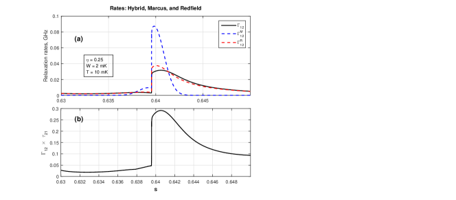
Figure 6: (a) At large coupling to the HF bath ($\eta=0.25$) and at a small interaction with the LF noise ($W=$ 2 mK), the hybrid rate $\Gamma_{12}$ is close to the Bloch-Redfield rate $\Gamma_{12}^{R}$. (b) The perturbation parameter $\Gamma_{12}\,\tau_{21}$ is less than 0.3.

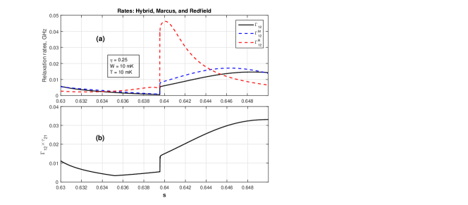
Figure 7: (a) When both couplings are large ($\eta=0.25$ and $W=10$ mK), the hybrid rate $\Gamma_{12}$, taken along the annealing path, deviates from Bloch-Redfield, $\Gamma_{12}^{R}$, and from Marcus, $\Gamma_{12}^{M},$ rates. (b) The perturbation parameter is small, $\Gamma_{12}\,\tau_{21}<0.04.$

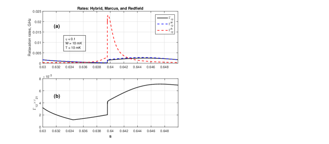
Figure 8: (a) At sufficiently large coupling of the system to the low-frequency bath, where $W=10$ mK, and at small coupling to the high-frequency bath, with $\eta=0.1$, the hybrid rate $\Gamma_{12}$ is close to the Marcus expression $\Gamma_{12}^{M}.$ (b) The perturbation parameter is decreasing in this case: $\Gamma_{12}\,\tau_{21}<0.01.$

In Fig. 9, in parallel with the energy spectrum, we plot a time dependence of the probabilities $P_{1}$ and $P_{2}$ to find the 16-qubit system in the instantaneous eigenstates $|1\rangle$ and $|2\rangle$ of the Hamiltonian $H_{S}$ (18).

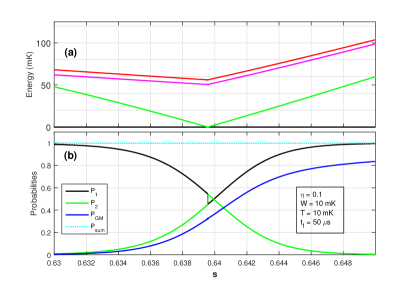
Figure 9: (a) Instantaneous energy spectrum of the 16-qubit system near the anticrossing point. (b) The evolution of the probabilities $P_{1},P_{2}$ to find the system in the instantaneous energy eigenstates during the annealing process at the total anneal time $t_{f}=2$ ms and at $\eta=0.1,W=10$ mK$,T=10$ mK. We also show the time evolution of the probability $P_{\rm GM}$ for the system to be in the $|GM\rangle$.

To calculate these probabilities, we obtain the numerical solution of the master equation (79) for the probabilities $P_{1^{\prime}}$ and $P_{2^{\prime}}$ to observe the system in the states $|1^{\prime}\rangle$ and $|2^{\prime}\rangle$ (VII.1). After that, we rotate the basis back, to the instantaneous energy eigenstates $|1\rangle$ and $|2\rangle.$ The contribution of the off-diagonal elements of the density matrix to the probabilities $P_{1}$ and $P_{2}$ rapidly disappears as it follows from Eqs. (VI.1) and (C.4). We also show the evolution of the probability $P_{\rm GM}$ (blue curve) to find the system in the state $|\rm GM\rangle$ defined in (VII). Here, we have a qualitative agreement with the experimental results shown in Fig. 2d of Ref. Dickson13 ).

References

- (1) A.J. Leggett, S. Chakravarty, A.T. Dorsey, M.P.A. Fisher, A. Garg, and W. Zwerger, Dynamics of the dissipative two-state system, Rev. Mod. Phys. 59, 1 (1987).
- (2) C.P. Slichter, Principles of magnetic resonance, 3rd ed. Springer-Verlag, Berlin, (1990).
- (3) D.F. Walls and G.J. Milburn, Quantum optics, Springer, New York, 1994.
- (4) T. Kadowaki and H. Nishimori, Quantum annealing in the transverse Ising model, Phys. Rev. E 58, 5355 (1998).
- (5) G.E. Santoro, R. Martonak, E. Tosatti, and R. Car, Theory of quantum annealing of an Ising spin glass, Science 295, 2427 (2002).
- (6) M.W. Johnson, M. H. S. Amin, S. Gildert, T. Lanting, F. Hamze, N. Dickson, R. Harris, A. J. Berkley, J. Johansson, P. Bunyk, E. M. Chapple, C. Enderud, J. P. Hilton, K. Karimi, E. Ladizinsky, N. Ladizinsky, T. Oh, I. Perminov, C. Rich, M. C. Thom, E. Tolkacheva, C. J. S. Truncik, S. Uchaikin, J. Wang, B. Wilson, and G. Rose, Quantum annealing with manufactured spins, Nature 473, 194 (2011).
- (7) E. Farhi, J. Goldstone, S. Gutmann, J. Lapan, A. Lundgren, and D. Preda, A quantum adiabatic evolution algorithm applied to random instances of an NP-complete problem, Science 292, 472 (2001).
- (8) S. Ashhab, J. R. Johansson, and Franco Nori, Decoherence in a scalable adiabatic quantum computer, Phys. Rev. A 74, 052330 (2006).
- (9) M.H.S. Amin, P.J. Love, and C.J.S. Truncik, Thermally assisted adiabatic quantum computation, 100, 060503 (2008).
- (10) T. Albash, S. Boixo, D. A. Lidar, and P. Zanardi, Quantum adiabatic Markovian master equations, New J. of Phys. 14 , 123016 (2012).
- (11) T. Albash and D.A. Lidar, Decoherence in adiabatic quantum computation Phys. Rev. A 91, 062320 (2015).
- (12) G.F. Efremov and A.Yu. Smirnov, Contribution to the microscopic theory of the fluctuations of a quantum system interacting with a Gaussian thermostat, Zh. Eksp. Teor. Fiz. 80, 1071 (1981) [Sov. Phys. JETP 53, 547 (1981)].
- (13) R. Harris, M. W. Johnson, T. Lanting, A. J. Berkley, J. Johansson, P. Bunyk, E. Tolkacheva, E. Ladizinsky, N. Ladizinsky, T. Oh, F. Cioata, I. Perminov, P. Spear, C. Enderud, C. Rich, S. Uchaikin, M. C. Thom, E. M. Chapple, J. Wang, B. Wilson, M. H. S. Amin, N. Dickson, K. Karimi, B. Macready, C. J. S. Truncik, and G. Rose, Experimental investigation of an eight qubit unit cell in a superconducting optimization processor, Phys. Rev. B 82, 024511 (2010).
- (14) R.A. Marcus, Electron transfer reactions in chemistry: Theory and experiment, Rev. Mod. Phys. 65, 599 (1993).
- (15) D.A. Cherepanov, L.I. Krishtalik, and A.Y. Mulkidjanian, Photosynthetic electron transfer controlled by protein relaxation: analysis by Langevin stochastic approach, Biophysical Journal 80, 1033 (2001).
- (16) A.Yu. Smirnov and M.H. Amin, Quantum eigenstate tomography with qubit tunneling spectroscopy, Low Temperature Physics (Fizika Nizkikh Temperatur), 43, 969 (2017).
- (17) M.H.S. Amin and D.V. Averin, Macroscopic resonant tunneling in the presence of low frequency noise, Phys. Rev. Lett. 100, 197001 (2008).
- (18) M.H.S. Amin and F. Brito, Non-Markovian incoherent quantum dynamics of a two-state system, Phys. Rev. B 80, 214302 (2009).
- (19) T. Lanting, M.H.S. Amin, M.W. Johnson, F. Altomare, A.J. Berkley, S. Gildert, R. Harris, J. Johansson, P. Bunyk, E. Ladizinsky, E. Tolkacheva, and D.V. Averin, Probing high-frequency noise with macroscopic resonant tunneling , Phys. Rev. B 83, 180502 (2011).
- (20) S. Boixo, V.N. Smelyanskiy, A. Shabani, S.V. Isakov, M. Dykman, V.S. Denchev, M.H. Amin, A.Yu. Smirnov, M. Mohseni, and H. Neven, Computational multiqubit tunnelling in programmable quantum annealers, Nature Communications 7,10327 (2016).
- (21) S. Boixo, V.N. Smelyanskiy, A. Shabani, S.V. Isakov, M. Dykman, V.S. Denchev, M.H. Amin, A.Yu. Smirnov, M. Mohseni, and H. Neven, Computational role of collective tunneling in a quantum annealer, arXiv:1411.4036v2 [quant-ph] (2015).
- (22) M. Yang and G.R. Fleming, Influence of phonons on exciton transfer dynamics: comparison of the Redfield, Förster, and modified Redfield equations, Chemical Physics 282, 163 (2002).
- (23) P.K. Ghosh, A.Yu. Smirnov, and F. Nori, Quantum effects in energy and charge transfer in an artificial photosynthetic complex, J. Chem. Phys. 134, 244103 (2011).
- (24) N. Lambert, Y.-N. Chen, Y.-C. Cheng, C.-M. Li, G.-Y. Chen, and F. Nori, Quantum biology, Nature Physics 9, 10 (2013).
- (25) R. Harris, M.W. Johnson, S. Han, A.J. Berkley, J. Johansson, P. Bunyk, E. Ladizinsky, S. Govorkov, M.C. Thom, S. Uchaikin, B. Bumble, A. Fung, A. Kaul, A. Kleinsasser, M.H.S. Amin, and D.V. Averin, Probing noise in flux qubits via macroscopic resonant tunneling, Phys. Rev. Lett. 101, 117003 (2008).
- (26) T. Lanting, A.J. Przybysz, A. Yu. Smirnov, F.M. Spedalieri, M.H. Amin, A.J. Berkley, R. Harris, F. Altomare, S. Boixo, P. Bunyk, N. Dickson, C. Enderud, J.P. Hilton, E. Hoskinson, M.W. Johnson, E. Ladizinsky, N. Ladizinsky, R. Neufeld, T. Oh, I. Perminov, C. Rich, M.C. Thom, E. Tolkacheva, S. Uchaikin, A.B. Wilson, G. Rose, Entanglement in a quantum annealing processor, Phys. Rev. X 4, 021041 (2014).
- (27) N.G. Dickson, M.W. Johnson, M.H. Amin, R. Harris, F. Altomare, A.J. Berkley, P. Bunyk, J. Cai, E.M. Chapple, P. Chavez, F. Cioata, T. Cirip, P. deBuen, M. Drew-Brook, C. Enderud, S. Gildert, F. Hamze, J. P. Hilton, E. Hoskinson, K. Karimi, E. Ladizinsky, N. Ladizinsky, T. Lanting, T. Mahon, R. Neufeld, T. Oh, I. Perminov, C. Petroff, A. Przybysz, C. Rich, P. Spear, A. Tcaciuc, M. C. Thom, E. Tolkacheva, S. Uchaikin, J. Wang, A.B. Wilson, Z. Merali and G. Rose, Thermally assisted quantum annealing of a 16-qubit problem, Nature Communications 4, 1903 (2013).
- (28) T. Lanting, R. Harris, J. Johansson, M. H. S. Amin, A. J. Berkley, S. Gildert, M. W. Johnson, P. Bunyk, E. Tolkacheva, E. Ladizinsky, N. Ladizinsky, T. Oh, I. Perminov, E. M. Chapple, C. Enderud, C. Rich, B. Wilson, M. C. Thom, S. Uchaikin, and G. Rose, Cotunneling in pairs of coupled flux qubits, Phys. Rev. B 82, 060512 (2010).
- (29) K. Blum, Density matrix theory and applications, 3rd ed. Springer-Verlag, Berlin, (2012).
- (30) N.G. Dickson, Elimination of perturbative crossings in adiabatic quantum optimization, New J. Phys. 13, 073011 (2011).
- (31) T. Lanting, A.D. King, B. Evert, and E. Hoskinson, Experimental demonstration of perturbative anticrossing mitigation using nonuniform driver Hamiltonians, Phys. Rev. A 96, 042322 (2017).
- (32) W.H. Zurek, Decoherence, einselection, and the quantum origins of the classical, Rev. Mod. Phys. 75, 715 (2003).
- (33) E. Gibney, Quantum computer gets design upgrade, Nature 541, 447 (2017).
- (34) M. Mohseni, P. Read, H. Neven, S. Boixo, V. Denchev, R. Babbush, A. Fowler, V. Smelyanskiy, and J. Martinis, Commercialize quantum technologies in five years, Nature 543, 171 (2017).
- (35) N. N. Bogoliubov and D. V. Shirkov, Quantum fields, Benjamin-Cummings Pub. Co., 1982.
- (36) V.I. Klyatskin, Dynamics of stochastic systems, Elsevier B.V., Amsterdam, 2005.