The electromagnetic multipole moments of the charged open-flavor $Z_{\bar{c}q}$ states

Abstract

The electromagnetic multipole moments of the open-flavor $Z_{\bar{c}q}$ states are investigated by assuming a diquark-antidiquark picture for their internal structure and quantum numbers $J^{PC}=1^{+-}$ for their spin-parity. In particular, their magnetic and quadrupole moments are extracted in the framework of light-cone QCD sum rule by the help of the photon distribution amplitudes. The electromagnetic multipole moments of the open-flavor $Z_{\bar{c}q}$ states are important dynamical observables, which encode valuable information on their underlying structure. The results obtained for the magnetic moments of different structures are considerably large and can be measured in future experiments. We obtain very small values for the quadrupole moments of $Z_{\bar{c}q}$ states indicating a nonspherical charge distribution.

I Introduction

Since 2003, there are many non-conventional hadrons discovered experimentally, such as many XYZ tetraquarks, $P_{c}^{+}(4380)$ and $P_{c}^{+}(4450)$ pentaquarks etc., which could not be described as the conventional hadrons composed of two or three valence quark/antiquarks. They are called exotic hadrons. For some reviews on the theoretical and experimental progress on the properties of these new states see Refs. Nielsen et al. (2010); Swanson (2006); Voloshin (2008); Klempt and Zaitsev (2007); Godfrey and Olsen (2008); Faccini et al. (2012); Esposito et al. (2015); Chen et al. (2016); Ali et al. (2017); Esposito et al. (2016); Olsen et al. (2017). The greatest achievement with regard to the exotic states was the discovery of the charged multiquark states. The charged states with a hidden pair of heavy quark and antiquark such as the $Z_{c}^{\pm}(3900)$ Ablikim et al. (2013a), $Z_{c}^{\pm}(4020)$ Ablikim et al. (2013b), $Z_{c}^{\pm}(4430)$ Choi et al. (2008), $Z_{b}^{\pm}(10610,10650)$ Bondar et al. (2012), would be undoubtedly considered as the exotic resonances, because these charged states cannot be explained as excited charmonium-like or bottomonium-like states.

Most of the discovered exotic states up to now share a common properties: they contain a hidden heavy quark-antiquark pair, $\bar{c}c$ or $\bar{b}b$. However existence of the multiquarks, which do not contain $\bar{c}c$ or $\bar{b}b$ pairs is also possible, because fundamental laws of QCD do not prohibit existence of such open-flavor multiquark states. It should be noted that they have not been discovered experimentally, and to our best knowledge, there are not any candidates to be considered for these states. They may be seen in the exclusive reactions as the open-charm and open-bottom resonances. In 2003, the two narrow charm-strange mesons $D^{∗}_{s0}(2317)$ and $D_{s1}(2460)$ were observed in the $D^{+}_{s}\pi^{0}$ and $D^{*+}_{s}\pi^{0}$ invariant mass distributions by the BABAR Aubert et al. (2003) and CLEO Besson et al. (2003)] collaborations, are now being considered as candidates to open-charm tetraquark states. In 2016, the D0 Collaboration reported the observation of a state with four different quark flavors, the $X(5568)$, and assigned the quantum numbers $J^{P}=0^{+}$ for it, but they did not exclude the possibility of $J^{P}=1^{+}$ Abazov et al. (2016). Reported in the $B^{0}_{s}\pi^{\pm}$ final states, the $X(5568)$ meson, if exist, cannot be categorized into the conventional meson family, and is a good candidate of exotic tetraquark state with valence quarks of four different flavors such as $su\bar{d}\bar{b}$ or $sd\bar{u}\bar{b}$. The observation of these states have immediately inspired extensive discussions on the possibility of their internal structure. For more information see for instance Refs. Agaev et al. (2016a, b); Chen et al. (2017a) and references therein. In 2017, the D0 Collaboration repeated their analysis when the $B_{s}$ is reconstructed semileptonically. They reported evidence for a narrow structure, which was consistent with their previous measurement in the hadronic decay mode Abazov et al. (2017). However, other experimental groups, namely the LHCb Aaij et al. (2016), CDF Aaltonen et al. (2017), CMS Sirunyan et al. (2017) and ATLAS Aaboud et al. (2018) collaborations could not find this resonance from analysis of their experimental data.

In order to understand the inner structure of the hadrons in the nonperturbative regime of QCD, the main challenges are the determination of the dynamical and statical features of hadrons such as their decay form factors, masses, electromagnetic multipole moments and so on, both experimentally and theoretically. Many theoretical models accurately estimate the mass and decay width of the discovered exotic states, but the inner structure of these states is still unclear. In other words, the mass and decay width alone can not distinguish the inner structure of the exotic states. Recall that the electromagnetic multipole moments are equally important dynamical observables of the exotic states. The electromagnetic multipole moments include the spatial distributions of the charge and magnetization in the hadrons and these parameters are directly related to the spatial distributions of quarks and gluons inside the hadrons. There are many studies in the literature devoted to the investigation of the electromagnetic multipole moments of the standard hadrons, but unfortunately relatively little are known the electromagnetic multipole moments of the exotic hadrons. There are a few studies in the literature where the magnetic dipole and quadrupole moments of the exotic states are studied: see  Agamaliev et al. (2017); Ozdem and Azizi (2017, 2018) for tetraquarks and  Kim and Praszalowicz (2004); Huang et al. (2004); Liu et al. (2004); Wang et al. (2005, 2006, 2016) for pentaquarks. More detailed analyses are needed in order to get useful knowledge on the charge distribution, electromagnetic multipole moments and geometric shapes of the non-conventional hadrons. In this study, we are going to concentrate on the charged open-flavor $[qq][\overline{qc}]$ states (hereafter we will denote these states as $Z_{\bar{c}q}$) with spin-parity $J^{PC}=1^{+-}$, and calculate their electromagnetic multipole moments in the framework of light-cone QCD sum rule (LCSR). In LCSR, the hadronic parameters are expressed in terms of the vacuum condensates and the light cone distribution amplitudes (DAs) of the on-shell particles (for more about this method see, e.g., Chernyak and Zhitnitsky (1990); Braun and Filyanov (1989); Balitsky et al. (1989) and references therein).

The rest of the paper is organized as follows: In section II, the calculation of the sum rules in LCSR will be presented. In the last section, we numerically analyze the sum rules obtained for the multipole moments and discuss the obtained results. The explicit expressions of the magnetic and quadrupole moments are moved to the Appendix A.

II Formalism

In this section we derive the LCSR for the magnetic and quadrupole moments of the $Z_{\bar{c}q}$ states. For this aim, we consider a correlation function in the presence of the external electromagnetic field ($\gamma$),

$$\Pi_{\mu\nu}(q)=i\int d^{4}xe^{ip\cdot x}\langle 0|\mathcal{T}\{J_{\mu}^{Z_{\bar{c}q}}(x)J_{\nu}^{Z_{\bar{c}q}\dagger}(0)\}|0\rangle_{\gamma},$$ (1)

where $J_{\mu}$ is the interpolating current of $Z_{\bar{c}q}$ state with quantum numbers $J^{PC}=1^{+-}$ in the diquark-antidiquark picture. It is given in terms of three light quark and one heavy quark fields as Chen et al. (2017b):

$$J_{\mu}^{Z_{\bar{c}q}}(x) = \Big{[}q_{1_{a}}^{T}(x)C\gamma_{\mu}q_{2_{b}}(x)\Big{]}\Big{[}\bar{q}_{3_{a}}(x)\gamma_{5}C\bar{c}_{b}^{T}(x)-\bar{q}_{3_{b}}(x)\gamma_{5}C\bar{c}_{a}^{T}(x)\Big{]},$$ (2)

where $q_{1}$ is u, d and/or s-quark, $q_{2}$ and $q_{3}$ are u and/or d-quark, $C$ is the charge conjugation matrix; and $a$ and $b$ are color indices.

In order to acquire sum rules for the magnetic and quadrupole moments, we need to represent the correlation function in two different forms: (1) in terms of the quark-gluon parameters and distribution amplitudes (DAs) of the photon in the deep Euclidean region, so called the QCD representation, and (2) in terms of hadronic properties, so called the hadronic representation.

We start our analysis by calculating the correlation function on Eq. (1) in terms of quarks and gluon properties in deep Euclidean region. For this purpose, the interpolating current is inserted into the correlation function and after the contracting of light and heavy quark pairs using the Wick theorem the following result is obtained:

$$\Pi_{\mu\nu}^{\mathrm{QCD}}(q)=i\int d^{4}xe^{ipx}\langle 0|\Bigg{\{}\mathrm{Tr}\Big{[}\gamma_{5}\widetilde{S}_{c}^{b^{\prime}b}(-x)\gamma_{5}S_{q_{3}}^{a^{\prime}a}(-x)\Big{]}\mathrm{Tr}\Big{[}\gamma_{\nu}\widetilde{S}_{q_{1}}^{aa^{\prime}}(x)\gamma_{\mu}S_{q_{2}}^{bb^{\prime}}(x)\Big{]}$$

$$-\mathrm{Tr}\Big{[}\gamma_{5}\widetilde{S}_{c}^{a^{\prime}b}(-x)\gamma_{5}S_{q_{3}}^{b^{\prime}a}(-x)\Big{]}\mathrm{Tr}\Big{[}\gamma_{\nu}\widetilde{S}_{q_{1}}^{aa^{\prime}}(x)\gamma_{\mu}S_{q_{2}}^{bb^{\prime}}(x)\Big{]}$$

$$-\mathrm{Tr}\Big{[}\gamma_{5}\widetilde{S}_{c}^{b^{\prime}a}(-x)\gamma_{5}S_{q_{3}}^{a^{\prime}b}(-x)\Big{]}\mathrm{Tr}\Big{[}\gamma_{\nu}\widetilde{S}_{q_{1}}^{aa^{\prime}}(x)\gamma_{\mu}S_{q_{2}}^{bb^{\prime}}(x)\Big{]}$$

$$+\mathrm{Tr}\Big{[}\gamma_{5}\widetilde{S}_{c}^{a^{\prime}a}(-x)\gamma_{5}S_{q_{3}}^{b^{\prime}b}(-x)\Big{]}\mathrm{Tr}\Big{[}\gamma_{\nu}\widetilde{S}_{q_{1}}^{aa^{\prime}}(x)\gamma_{\mu}S_{q_{2}}^{bb^{\prime}}(x)\Big{]}\Bigg{\}}|0\rangle_{\gamma},$$ (3)

where

$$\widetilde{S}(x)=CS^{\mathrm{T}}(x)C,$$

with $S_{q,c}(x)$ being the quark propagators. The light and heavy propagators are given as Balitsky and Braun (1989)

$$S_{q}(x)=S^{free}-\frac{\langle\bar{q}q\rangle}{12}\Big{(}1-i\frac{m_{q}x\!\!\!/}{4}\Big{)}-\frac{\langle\bar{q}q\rangle}{192}m_{0}^{2}x^{2}\Big{(}1-i\frac{m_{q}x\!\!\!/}{6}\Big{)}-\frac{ig_{s}}{32\pi^{2}x^{2}}~{}G^{\mu\nu}(x)\Bigg{[}\hbox to0.0pt{/\hss}{x}\sigma_{\mu\nu}+\sigma_{\mu\nu}\hbox to0.0pt{/\hss}{x}\Bigg{]},$$ (4)

and

$$S_{c}(x)=S^{free}-\frac{g_{s}m_{c}}{16\pi^{2}}\int_{0}^{1}dv~{}G^{\mu\nu}(vx)\Bigg{[}(\sigma_{\mu\nu}{x\!\!\!/}+{x\!\!\!/}\sigma_{\mu\nu})\frac{K_{1}(m_{c}\sqrt{-x^{2}})}{\sqrt{-x^{2}}}+2\sigma^{\mu\nu}K_{0}(m_{c}\sqrt{-x^{2}})\Bigg{]},$$ (5)

where

$$S_{q}^{free}(x)=i\frac{{x\!\!\!/}}{2\pi^{2}x^{4}}-\frac{m_{q}}{4\pi^{2}x^{2}},$$

$$S_{c}^{free}(x)=\frac{m_{c}^{2}}{4\pi^{2}}\Bigg{[}\frac{K_{1}(m_{c}\sqrt{-x^{2}})}{\sqrt{-x^{2}}}+i\frac{{x\!\!\!/}~{}K_{2}(m_{c}\sqrt{-x^{2}})}{(\sqrt{-x^{2}})^{2}}\Bigg{]}.$$ (6)

Here $K_{1,2}$ are Bessel functions of the second kind.

The correlation function contains different types of contributions. In first part, one of the free quark propagators in Eq. (II) is replaced by

$$S^{free}(x)\rightarrow\int d^{4}y\,S^{free}(x-y)\,\hbox to0.0pt{/\hss}{\!A}(y)\,S^{free}(y)\,,$$ (7)

and the remaining three propagators are taken as the full quark propagators.

In the second case one of the light quark propagators in Eq. (II) is replaced by

$$S_{\alpha\beta}^{ab}\rightarrow-\frac{1}{4}(\bar{q}^{a}\Gamma_{i}q^{b})(\Gamma_{i})_{\alpha\beta},$$ (8)

and the remaining propagators are taken as the full quark propagators, as well including the perturbative and the nonperturbative contributions. Once Eq. (8) is plugged into Eq. (II), there appear matrix elements such as $\langle\gamma(q)\left|\bar{q}(x)\Gamma_{i}q(0)\right|0\rangle$ and $\langle\gamma(q)\left|\bar{q}(x)\Gamma_{i}G_{\alpha\beta}q(0)\right|0\rangle$, representing the nonperturbative contributions. The reader can find some details about the transformations of Eqs. (7) and (8) in Ref. Ozdem and Azizi (2018). These matrix elements can be written in terms of the photon DAs with definite twists, whose expressions all can be found in Ref. Ball et al. (2003). The QCD side of the correlation function can be acquired in terms of QCD parameters using the Eqs. (II)-(8) and after applying the Fourier transformation to transfer the calculations to the momentum space.

The next step is to calculate the correlation function in terms of the hadronic parameters. To this end we insert intermediate states of $Z_{\bar{c}q}$ with the same quantum numbers as the interpolating current into Eq. (1). As a result, in zero-width approximation, we get

$$\Pi_{\mu\nu}^{Had}(p,q)={\frac{\langle 0\mid J_{\mu}^{Z_{\bar{c}q}}\mid Z_{\bar{c}q}(p)\rangle}{[p^{2}-m_{Z_{\bar{c}q}}^{2}]}}\langle Z_{\bar{c}q}(p)\mid Z_{\bar{c}q}(p+q)\rangle_{\gamma}\frac{\langle Z_{\bar{c}q}(p+q)\mid{J^{\dagger}}_{\nu}^{Z_{\bar{c}q}}\mid 0\rangle}{[(p+q)^{2}-m_{Z_{\bar{c}q}}^{2}]}+\cdots,$$ (9)

where dots stand for the contributions of the higher and continuum states and $q$ is the momentum of the photon. The matrix element $\langle 0\mid J_{\mu}^{Z_{\bar{c}q}}\mid Z_{\bar{c}q}\rangle$ is determined as

$$\langle 0\mid J_{\mu}^{Z_{\bar{c}q}}\mid Z_{\bar{c}q}\rangle=\lambda_{Z_{\bar{c}q}}\varepsilon_{\mu}^{\theta}\,,$$ (10)

with $\lambda_{Z_{\bar{c}q}}$ being the residue of the $Z_{\bar{c}q}$ state.

The matrix element $\langle Z_{\bar{c}q}(p,\varepsilon^{\theta})\mid Z_{\bar{c}q}(p+q,\varepsilon^{\delta})\rangle_{\gamma}$ can be written in terms of three Lorentz invariant form factors as follows Brodsky and Hiller (1992):

$$\langle Z_{\bar{c}q}(p,\varepsilon^{\theta})\mid Z_{\bar{c}q}(p+q,\varepsilon^{\delta})\rangle_{\gamma} =-\varepsilon^{\tau}(\varepsilon^{\theta})^{\alpha}(\varepsilon^{\delta})^{\beta}\Bigg{[}G_{1}(Q^{2})~{}(2p+q)_{\tau}~{}g_{\alpha\beta}+G_{2}(Q^{2})~{}(g_{\tau\beta}~{}q_{\alpha}-g_{\tau\alpha}~{}q_{\beta})$$

$$-\frac{1}{2m_{Z_{\bar{c}q}}^{2}}G_{3}(Q^{2})~{}(2p+q)_{\tau}~{}q_{\alpha}q_{\beta}\Bigg{]}\,,$$ (11)

where $\varepsilon^{\theta}$ and $\varepsilon^{\delta}$ are the polarization vectors of the initial and final $Z_{\bar{c}q}$ states and $\varepsilon^{\tau}$ is the polarization vector of the photon. The Lorentz invariant form factors $G_{1}(Q^{2})$, $G_{2}(Q^{2})$ and $G_{3}(Q^{2})$ are related to the charge, magnetic and quadrupole form factors through the relations

$$F_{C}(Q^{2})=G_{1}(Q^{2})+\frac{2}{3}\eta F_{\cal D}(Q^{2})\,,$$

$$F_{M}(Q^{2})=G_{2}(Q^{2})\,,$$

$$F_{\cal D}(Q^{2})=G_{1}(Q^{2})-G_{2}(Q^{2})+(1+\eta)G_{3}(Q^{2})\,,$$ (12)

where $\eta=Q^{2}/4m_{Z_{\bar{c}q}}^{2}$ with $Q^{2}=-q^{2}$. At $Q^{2}=0$, these form factors are corresponding to the electric charge, magnetic moment $\mu$ and the quadrupole moment ${\cal D}$ as:

$$eF_{C}(0)=e\,,$$

$$eF_{M}(0)=2m_{Z_{\bar{c}q}}\mu\,,$$

$$eF_{\cal D}(0)=m_{Z_{\bar{c}q}}^{2}{\cal D}\,.$$ (13)

Using Eqs. (10)-(II) and imposing the condition $q\!\cdot\!\varepsilon=0$ the Eq. (9) takes the form,

$$\Pi_{\mu\nu}^{Had} =\frac{\lambda_{Z_{\bar{c}q}}^{2}}{[m_{Z_{\bar{c}q}}^{2}-(p+q)^{2}][m_{Z_{\bar{c}q}}^{2}-p^{2}]}\Bigg{[}2(p.\varepsilon)F_{C}(0)\Bigg{(}g_{\mu\nu}-\frac{p_{\mu}q_{\nu}-p_{\nu}q_{\mu}}{m_{Z_{\bar{c}q}}^{2}}\Bigg{)}$$

$$+F_{M}(0)\Bigg{(}q_{\mu}\varepsilon_{\nu}-q_{\nu}\varepsilon_{\mu}+\frac{1}{m_{Z_{\bar{c}q}}^{2}}(p.\varepsilon)(p_{\mu}q_{\nu}-p_{\nu}q_{\mu})\Bigg{)}-\Bigg{(}F_{C}(0)+F_{\cal D}(0)\Bigg{)}{\frac{p.\varepsilon}{m_{Z_{\bar{c}q}}^{2}}}q_{\mu}q_{\nu}\Bigg{]}\,,$$ (14)

where we inserted

$$\sum_{\lambda}\varepsilon_{\mu}(p,\lambda)\varepsilon_{\nu}(p,\lambda)=-g_{\mu\nu}+\frac{p_{\mu}p_{\nu}}{m_{Z_{\bar{c}q}}^{2}}.$$ (15)

Equating the QCD and hadronic sides of the correlation function, we obtain the expression of the electromagnetic multipole moments in LCSR in terms of the QCD degrees of freedom and the photon DAs. We perform the double Borel transforms with respect to the variables $p^{2}$ and $(p+q)^{2}$ on both sides of the correlation function in order to suppress the contributions of the higher states and continuum, and use the quark-hadron duality assumption. By matching the coefficients of the structures $q_{\mu}\varepsilon_{\nu}$ and $(\varepsilon.p)q_{\mu}q_{\nu}$, respectively for the magnetic and quadrupole moments, we get

$$\mu=\frac{e^{m_{Z_{\bar{c}q}}^{2}/M^{2}}}{\lambda_{Z_{\bar{c}q}}^{2}}\Pi_{1}^{QCD},$$

$$\mathcal{D}=m^{2}_{Z_{\bar{c}q}}\frac{e^{m_{Z_{\bar{c}q}}^{2}/M^{2}}}{\lambda_{Z_{\bar{c}q}}^{2}}\Pi_{2}^{QCD},$$ (16)

where explicit expressions of the $\Pi_{1}^{QCD}$ and $\Pi_{2}^{QCD}$ are given in Appendix A.

III Numerical analysis

In this section, we numerically analyze the results of calculations for magnetic and quadrupole moments. We use $m_{u}=m_{d}=0$, $m_{s}(2~{}GeV)=0.096^{+0.008}_{-0.004}~{}GeV$, $\overline{m}_{c}(m_{c})=(1.28\pm 0.03)\,GeV$ Patrignani et al. (2016), $\langle\bar{u}u\rangle(1~{}GeV)=\langle\bar{d}d\rangle(1~{}GeV)=(-0.24\pm 0.01)^{3}~{}GeV^{3}$ Ioffe (2006), $m_{0}^{2}=0.8\pm 0.1~{}GeV^{2}$, $\langle g_{s}^{2}G^{2}\rangle=0.88~{}GeV^{4}$ Nielsen et al. (2010), $\chi(1~{}GeV)=-2.85\pm 0.5~{}GeV^{-2}$ Rohrwild (2007), $\lambda_{Z_{sq\bar{q}c}}=7.3\pm 1.7\times 10^{-3}~{}GeV^{5}$, $\lambda_{Z_{qq\bar{q}c}}=7.6\pm 1.8\times 10^{-3}~{}GeV^{5}$, $m_{Z_{sq\bar{q}c}}=2.826^{+0.134}_{-0.157}~{}GeV$ and $m_{Z_{qq\bar{q}c}}=2.843^{+0.115}_{-0.139}~{}GeV$ Agaev et al. (2017). The parameters used in the photon DAs are given in Ref. Ball et al. (2003).

The predictions for the electromagnetic multipole moments depend on two auxiliary parameters; the Borel mass parameter $M^{2}$ and continuum threshold $s_{0}$. Complying with the standard procedure of the sum rule method the predictions on the electromagnetic multipole moments should not depend on $M^{2}$ and $s_{0}$, but in real computations one can only decrease their effect to a minimum. The working interval for the continuum threshold is chosen such that the maximum pole contribution is acquired and the results relatively weakly depend on its choices. Our numerical computations lead to the interval [10-12] $GeV^{2}$ for this parameter. The working region for $M^{2}$ is determined requiring that the contributions of the higher states and continuum are effectively suppressed. There are two criteria for choosing working region for the Borel parameter $M^{2}$: Convergence of the operator product expansion (OPE) and pole dominance. The requirement of the OPE convergence results in a lower bound, while the constraint of the maximum pole contribution leads to an upper bound on it. Our numerical calculation shows that these requirements are satisfied in the region $3~{}GeV^{2}\leq M^{2}\leq 4~{}GeV^{2}$ and, the magnetic and quadrupole moments in this region is practically independent of $M^{2}$. In Figs. 1-2, we plot the dependencies of the magnetic and quadrupole moments on $M^{2}$ at several fixed values of the continuum threshold $s_{0}$. As is seen, the variation of the results with respect to the continuum threshold causes a change on the results on the magnetic and quadrupole moments of about 15% and there is a very less dependence of the quantities under consideration on the Borel parameter in its working interval. Hence, one can say that the results of the magnetic and quadrupole moments are almost insensitive to $s_{0}$ and $M^{2}$.

Our final results for the magnetic and quadrupole moments are given in Table I. The errors in the results come from the variations in the calculations of the working regions of $M^{2}$ and $s_{0}$ as well as the uncertainties in the values of the input parameters and the photon DAs. We also would like to note that in Table I and Figs. 1-2, the absolute values are given since it is not possible to determine the sign of the residue from the mass sum rules. Therefore, it is not possible to estimate the signs of the magnetic and quadrupole moments.

${Z_{\bar{c}q}}$	$|\mu_{Z_{\bar{c}q}}|[\mu_{N}]$	$|\mathcal{D}_{Z_{\bar{c}q}}|[fm^{2}]$
$[sd][\overline{uc}]$	1.12$\pm$ 0.18	0.0086 $\pm$ 0.0015
$[sd][\overline{dc}]$	0.90$\pm$ 0.13	0.0085 $\pm$ 0.0015
$[su][\overline{uc}]$	0.51$\pm$ 0.24	0.0070 $\pm$ 0.0013
$[dd][\overline{uc}]$	1.09$\pm$ 0.17	0.0082 $\pm$ 0.0014
$[du][\overline{uc}]$	0.84$\pm$ 0.31	0.0067 $\pm$ 0.0012
$[dd][\overline{dc}]$	0.93$\pm$ 0.13	0.0082 $\pm$ 0.0014
$[uu][\overline{dc}]$	2.05$\pm$ 0.30	0.016$\pm$0.003

Table 1: Results of the magnetic and quadrupole moments of $Z_{\bar{c}q}$ states.

In summary, the electromagnetic multipole moments of the open-flavor $Z_{\bar{c}q}$ states have been investigated by assuming that these states are represented as diquark-antidiquark structure with quantum numbers $J^{PC}=1^{+-}$. Their magnetic and quadrupole moments have been extracted in the framework of light-cone QCD sum rule. The electromagnetic multipole moments of the open-flavor $Z_{\bar{c}q}$ states are important dynamical observables, which would encode important information of their underlying structure, charge distribution and geometric shape. The results obtained for the magnetic moments are considerably large and can be measured in future experiments. We obtain very small values for the quadrupole moments of $Z_{\bar{c}q}$ states indicating a nonspherical charge distribution. It is easy to see that $[sd][\overline{uc}]$ and $[dd][\overline{uc}]$ states belong to a class of doubly charged tetraquarks that the measurements of their electromagnetic parameters, like those of the $\Delta^{++}$ baryon, are relatively easy compared to other exotic states. These kind of exotic states have not been observed so far. We hope our predictions on the electromagnetic moments of these states together with the results of other theoretical studies on the spectroscopic parameters of these states will be useful for their searches in future experiments and will hep us determine exact internal structures of these non-conventional states.

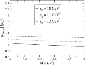
(a)

(b)

(c)

(d)

(e)

(f)

Figure 1: The dependence of the magnetic and quadrupole moments on the Borel parameter squared $M^{2}$ at different fixed values of the continuum threshold: (a) and (b) for the $Z_{sd\bar{u}\bar{c}}$ state, (c) and (d) for the $Z_{sd\bar{d}\bar{c}}$ state and, (e) and (f) for the $Z_{su\bar{u}\bar{c}}$ state.

(a)

(b)

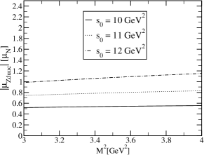
(c)

(d)

(e)

(f)

(g)

(h)

Figure 2: The dependence of the magnetic and quadrupole moments on the Borel parameter squared $M^{2}$ at different fixed values of the continuum threshold: (a) and (b) for the $Z_{dd\bar{u}\bar{c}}$ state, (c) and (d) for the $Z_{du\bar{u}\bar{c}}$ state, (e) and (f) for the $Z_{dd\bar{d}\bar{c}}$ state and, (g) and (h) for the $Z_{uu\bar{d}\bar{c}}$ state.

IV Acknowledgement

This work has been supported by the Scientific and Technological Research Council of Turkey (TÜBİTAK) under the Grant No. 115F183.

Appendix A: Explicit forms of the functions $\Pi_{i}^{QCD}$

In this appendix, we present the explicit expressions for the functions $\Pi_{1}^{QCD}$ and $\Pi_{2}^{QCD}$:

$$\Pi_{1}^{QCD} =\frac{1}{442368\pi^{2}}\Bigg{[}32P_{1}\Bigg{\{}eq_{3}mcP_{3}+144eq_{1}\pi^{2}P_{2}(m_{0}^{2}-m_{c}^{2})+3eq_{2}\Bigg{(}m_{q_{1}}P_{3}+12\Big{(}m_{c}^{2}m_{q_{1}}+8\pi^{2}m_{c}m_{q_{1}}P_{1}$$

$$+4\pi^{2}m_{0}^{2}P_{2}-8\pi^{2}m_{c}^{2}P_{2}\Big{)}\Bigg{)}\Bigg{\}}\mathbb{A}(u_{0})+64\chi P_{1}\Bigg{\{}8eq_{1}\pi^{2}P_{2}\Bigg{(}P_{3}+6m_{c}\Big{(}-3m_{c}m_{0}^{2}+2m_{c}^{3}+16\pi^{2}P_{1}\Big{)}\Bigg{)}$$

$$+eq_{2}\Bigg{(}P_{3}(3m_{c}^{2}m_{q_{1}}-8\pi^{2}P_{2})+48\pi^{2}m_{c}\Big{(}3m_{q_{1}}m_{0}^{2}P_{1}-3m_{c}m_{0}^{2}P_{2}+2m_{c}^{3}P_{2}+16\pi^{2}P_{1}P_{2}\Big{)}\Bigg{)}\Bigg{\}}\varphi_{\gamma}(u_{0})$$

$$+32f_{3\gamma}\Bigg{\{}-eq_{3}m_{c}^{2}P_{3}+3eq_{1}m_{c}\Big{(}m_{c}P_{3}+96\pi^{2}P_{1}(m_{0}^{2}-m_{c}^{2})\Big{)}+3eq_{2}\Bigg{(}-m_{c}^{2}P_{3}-48\pi^{2}\Big{(}m_{0}^{2}(2m_{c}P_{1}+m_{q_{1}}P_{2})$$

$$-m_{c}^{2}(2m_{c}P_{1}+3m_{q_{1}}P_{2})\Big{)}\Bigg{)}\Bigg{\}}\psi^{a}(u_{0})-1536\pi^{2}f_{3\gamma}\Bigg{\{}3eq_{1}m_{c}m_{0}^{2}P_{1}+eq_{2}\Big{(}-3m_{c}^{2}m_{q_{1}}P_{1}+m_{0}^{2}(3m_{c}P_{1}$$

$$+3m_{q_{1}}P_{2})\Big{)}\Bigg{\}}\Bigg{(}\psi^{\nu}(u_{0})+2I_{6}[\psi^{\nu}]\Bigg{)}+192P_{1}\Bigg{\{}24eq_{1}\pi^{2}P_{2}(m_{0}^{2}-2m_{c}^{2})+eq_{2}\Bigg{(}m_{q_{1}}P_{3}+24\pi^{2}\Big{(}4m_{c}m_{q_{1}}P_{1}$$

$$+m_{0}^{2}P_{2}-2m_{c}^{2}P_{2}\Big{)}\Bigg{)}\Bigg{\}}I_{6}[h_{\gamma}]+11eq_{3}m_{c}^{2}f_{3\gamma}P_{3}I_{2}[\mathcal{A}]+(eq_{1}-eq_{2})m_{c}f_{3\gamma}\Big{(}23m_{c}P_{3}+576\pi^{2}P_{1}(m_{0}^{2}-2m_{c}^{2})\Big{)}I_{1}[\mathcal{A}]$$

$$+576eq_{3}\pi^{2}m_{c}m_{q_{1}}P_{1}P_{2}\Big{(}2I_{5}[\mathcal{S}]+I_{2}[\mathcal{S}]\Big{)}-44eq_{3}m_{c}P_{1}P_{3}\Big{(}I_{4}[\mathcal{T}_{1}]+I_{5}[\mathcal{T}_{1}]\Big{)}$$

$$-240eq_{3}\pi^{2}m_{q_{1}}f_{3\gamma}P_{2}(m_{0}^{2}-3m_{c}^{2})I_{2}[\mathcal{V}]+(eq_{1}+eq_{2})m_{c}f_{3\gamma}\Big{(}-23m_{c}P_{3}-576\pi^{2}P_{1}(m_{0}^{2}-2m_{c}^{2})\Big{)}I_{1}[\mathcal{V}]\Bigg{]}I_{7}[0]$$

$$+\frac{1}{221184m_{c}^{2}\pi^{4}}\Bigg{[}-16m_{c}P_{1}\Bigg{\{}eq_{3}P_{3}+36m_{c}\Big{(}3eq_{2}m_{c}^{2}m_{q_{1}}-8(eq_{1}+eq_{2})\pi^{2}P_{2}\Big{)}\Bigg{\}}\mathbb{A}(u_{0})$$

$$+192m_{c}^{2}\chi P_{1}\Big{\{}-eq_{2}m_{q_{1}}P_{3}+96eq_{2}\pi^{2}m_{c}m_{q_{1}}P_{1}+24(eq_{1}+eq_{2})\pi^{2}P_{1}(m_{0}^{2}-2m_{c}^{2})\Bigg{\}}\varphi_{\gamma}(u_{0})$$

$$+32m_{c}f_{3\gamma}\Bigg{\{}(eq_{3}-3eq_{1})m_{c}P_{3}-72eq_{1}\pi^{2}P_{1}(m_{0}^{2}-4m_{c}^{2})+3eq_{2}\Bigg{(}m_{c}P_{3}+24\pi^{2}\Big{(}m_{0}^{2}P_{1}-4m_{c}(m_{c}P_{1}$$

$$+m_{q_{1}}P_{2})\Big{)}\Bigg{)}\Bigg{\}}\psi^{a}(u_{0})+2304\pi^{2}m_{c}f_{3\gamma}\Bigg{\{}(eq_{1}+eq_{2})m_{0}^{2}P_{1}-2eq_{2}m_{c}m_{q_{1}}P_{1}\Bigg{\}}\Bigg{(}\psi^{\nu}(u_{0})+2I_{6}[\psi^{\nu}]\Bigg{)}$$

$$+96P_{1}\Bigg{\{}96(eq_{1}+eq_{2})\pi^{2}m_{c}^{2}P_{2}+eq_{2}m_{q_{1}}\Big{(}P_{3}+96\pi^{2}m_{c}P_{1}\Big{)}\Bigg{\}}I_{6}[h_{\gamma}]+22eq_{3}m_{c}P_{1}P_{3}\Bigg{(}I_{5}[\mathcal{T}_{1}]+I_{5}[\mathcal{T}_{2}]\Bigg{)}$$

$$-288eq_{3}\pi^{2}m_{c}m_{q_{1}}P_{1}P_{2}I_{2}[\mathcal{S}]-11eq_{3}m_{c}^{2}f_{3\gamma}P_{3}I_{2}[\mathcal{A}]+(eq_{1}-eq_{2})m_{c}^{2}f_{3\gamma}\Big{(}-23P_{3}+1152\pi^{2}m_{c}P_{1}\Big{)}I_{1}[\mathcal{A}]$$

$$-432eq_{3}\pi^{2}m_{c}^{2}m_{q_{1}}f_{3\gamma}P_{2}I_{2}[\mathcal{V}]-(eq_{1}+eq_{2})m_{c}^{2}f_{3\gamma}\Big{(}-23P_{3}+1152\pi^{2}m_{c}P_{1}\Big{)}I_{1}[\mathcal{V}]\Bigg{]}I_{7}[1]$$

$$+\frac{1}{442368m_{c}^{2}\pi^{4}}\Bigg{[}3456eq_{2}m_{c}^{2}m_{q_{1}}P_{1}\mathbb{A}(u_{0})+192\chi P_{1}\Bigg{\{}96(eq_{1}+eq_{2})\pi^{2}m_{c}^{2}P_{2}+eq_{2}m_{q_{1}}\Big{(}P_{3}+96\pi^{2}m_{c}P_{1}\Big{)}\Bigg{\}}\varphi_{\gamma}(u_{0})$$

$$-32f_{3\gamma}\Bigg{\{}eq_{3}P_{3}+288eq_{1}\pi^{2}m_{c}P_{1}+3eq_{2}\Big{(}P_{3}+48\pi^{2}(2m_{c}P_{1}+msP_{2})\Big{)}\Bigg{\}}\psi^{a}(u_{0})+11eq_{3}f_{3\gamma}P_{3}I_{2}[\mathcal{A}]$$

$$-9216(eq_{1}+eq_{2})\pi^{2}P_{1}P_{2}I_{6}[h_{\gamma}]+2304eq_{2}\pi^{2}m_{q_{1}}f_{3\gamma}P_{2}I_{3}[\psi^{a}]+4608eq_{2}\pi^{2}m_{q_{1}}f_{3\gamma}P_{2}\Big{(}\psi^{\nu}(u_{0})+2I_{6}[\psi^{\nu}]\Big{)}$$

$$+(eq_{1}+eq_{2})f_{3\gamma}\Big{(}23P_{3}+1152\pi^{2}m_{c}P_{1}\Big{)}I_{1}[\mathcal{A}]+(eq_{1}+eq_{2})f_{3\gamma}\Big{(}-23P_{3}+1152\pi^{2}m_{c}P_{1}\Big{)}I_{1}[\mathcal{V}]$$

$$+144eq_{3}\pi^{2}m_{q_{1}}f_{3\gamma}P_{2}I_{2}[\mathcal{V}]\Bigg{]}I_{7}[2]$$

$$-\frac{eq_{3}m_{c}m_{q_{1}}P_{1}P_{2}P_{3}}{20736\pi^{4}}\Bigg{[}2\varphi_{\gamma}(u_{0})+I_{3}[\varphi_{\gamma}]\Bigg{]}I_{7}[-1]-\frac{P_{1}}{1152m_{c}^{2}\pi^{4}}\Bigg{[}16(eq_{1}+eq_{2})\pi^{2}\chi P_{2}\varphi_{\gamma}(u_{0})+3eq_{2}m_{q_{1}}\mathbb{A}(u_{0})\Bigg{]}I_{7}[3]$$

$$-\frac{m_{c}^{4}}{442368\pi^{4}}\Bigg{[}64eq_{3}m_{c}\chi P_{1}P_{3}\varphi_{\gamma}(u_{0})+64f_{3\gamma}\Bigg{\{}-eq3P_{3}+3eq_{1}\Big{(}P_{3}+96\pi^{2}m_{c}P_{1}\Big{)}+3eq_{2}\Big{(}-P_{3}+48\pi^{2}\big{(}2m_{c}P_{1}$$

$$-m_{q_{1}}P_{2}\big{)}\Big{)}\Bigg{\}}\Big{(}2\psi^{a}(u_{0})+I_{3}[\psi^{a}]\Big{)}-192f_{3\gamma}\Bigg{\{}(eq_{1}+eq_{2})\Big{(}P_{3}+96\pi^{2}m_{c}P_{1}\Big{)}-48eq_{2}\pi^{2}m_{q_{1}}P_{2}\Bigg{\}}\Big{(}\psi^{\nu}(u_{0})+2I_{6}[\psi^{\nu}]\Big{)}$$

$$+18432(eq_{1}+eq_{2})\pi^{2}P_{1}P_{2}I_{6}[h_{\gamma}]+32eq_{3}m_{c}\chi P_{3}P_{1}I_{3}[h_{\gamma}]-11eq_{3}f_{3\gamma}P_{3}I_{2}[\mathcal{A}]-288eq_{3}\pi^{2}m_{q_{1}}f_{3\gamma}P_{2}I_{2}[\mathcal{V}]\Bigg{]}I_{8}[-3,1]$$

$$+\frac{m_{c}^{2}}{442368\pi^{2}}\Bigg{[}-384eq_{2}m_{q_{1}}\chi P_{1}\Big{(}P_{3}+96\pi^{2}m_{c}P_{1}\Big{)}\varphi_{\gamma}(u_{0})-64eq_{3}m_{c}\chi P_{1}P_{3}I_{3}[\varphi_{\gamma}]-192(eq_{1}+eq_{2})f_{3\gamma}\Big{(}P_{3}$$

$$+96\pi^{2}m_{c}P_{1}\Big{)}\Big{(}\psi^{\nu}(u_{0})+2I_{6}[\psi^{\nu}]\Big{)}+32f_{3\gamma}\Bigg{\{}(3eq_{1}-3eq_{2}-eq_{3})P_{3}+288(eq_{1}-eq_{2})\pi^{2}m_{c}P_{1}\Bigg{\}}I_{3}[\psi^{a}]$$

$$-2(eq_{1}-eq_{2})f_{3\gamma}\Big{(}23P_{3}+1152\pi^{2}m_{c}P_{1}\Big{)}I_{1}[\mathcal{A}]+2(eq_{1}+eq_{2})f_{3\gamma}\Big{(}23P_{3}+1152\pi^{2}m_{c}P_{1}\Big{)}I_{1}[\mathcal{V}]$$

$$-33eq_{3}f_{3\gamma}P_{3}I_{2}[\mathcal{A}]\Bigg{]}I_{8}[-2,1]$$

$$+\frac{P_{1}}{110592m_{c}^{2}\pi^{4}}\Bigg{[}8eq_{3}m_{c}P_{3}A(u_{0})+576(eq_{1}-eq_{2})\pi^{2}m_{c}f_{3\gamma}m_{0}^{2}\Big{(}2\psi^{a}(u_{0})+I_{3}[\psi^{a}]\Big{)}+144eq_{3}\pi^{2}m_{c}m_{q_{1}}P_{2}I_{2}[\mathcal{S}]$$

$$-1152(eq_{1}+eq_{2})\pi^{2}m_{c}f_{3\gamma}m_{0}^{2}\Big{(}\psi^{\nu}(u_{0})+2I_{6}[\psi^{\nu}]\Big{)}+48eq_{2}m_{q_{1}}\Big{(}-P_{3}+96\pi^{2}m_{c}P_{1}\Big{)}I_{6}[h_{\gamma}]$$

$$-11eq_{3}m_{c}P_{3}\Big{(}I_{5}[\mathcal{T}_{1}]-I_{5}[\mathcal{T}_{2}]\Big{)}\Bigg{]}I_{8}[0,0]$$

$$-\frac{1}{221184m_{c}^{2}\pi^{4}}\Bigg{[}64\chi P_{1}\Bigg{\{}P_{3}(2eq_{3}m_{c}-3eq_{2}m_{q_{1}})+288\pi^{2}m_{c}m_{q_{1}}P_{1}\Bigg{\}}\varphi_{\gamma}(u_{0})+32f_{3\gamma}\Bigg{\{}3eq_{1}\Big{(}96\pi^{2}m_{c}P_{1}-P_{3}\Big{)}+eq_{3}P_{3}$$

$$+3eq_{2}\Big{(}P_{3}+48\pi^{2}(2m_{c}P_{1}+m_{q_{1}}P_{2})\Big{)}\Bigg{\}}\Big{(}\psi^{a}(u_{0})-2I_{3}[\psi^{a}]\Big{)}-4608eq_{2}\pi^{2}m_{q_{1}}f_{3\gamma}P_{2}\Big{(}\psi^{\nu}(u_{0})+2I_{6}[\psi^{\nu}]\Big{)}$$

$$-9216eq_{2}\pi^{2}P_{1}P_{2}I_{6}[h_{\gamma}]\Bigg{]}I_{8}[0,1]$$

$$+\frac{1}{1536m_{c}^{2}\pi^{4}}\Bigg{[}32eq_{2}m_{q_{1}}\chi P_{1}\varphi_{\gamma}(u_{0})+16(eq_{1}+eq_{2})f_{3\gamma}\Big{(}\psi^{\nu}(u_{0})+2I_{6}[\psi^{\nu}]\Big{)}-8(eq_{1}-eq_{2})f_{3\gamma}I_{3}[\psi^{a}]$$

$$+f{3\gamma}\Big{\{}2(eq_{1}-eq_{2})I_{1}[\mathcal{A}]-eq_{3}I_{2}[\mathcal{V}]-2(eq_{1}+eq_{2})I_{1}[\mathcal{V}]\Big{\}}\Bigg{]}I_{8}[0,3]$$

$$+\frac{m_{c}^{4}}{6144\pi^{4}}\Bigg{[}64eq_{2}m_{q_{1}}\chi P_{1}\Big{(}m_{c}^{2}F[-4,3]+I_{8}[-3,3]\Big{)}\varphi_{\gamma}(u_{0})-16(eq_{1}-eq_{2})f_{3\gamma}\Big{(}m_{c}^{4}F[-5,3]+I_{8}[-3,3]\Big{)}\psi^{a}(u_{0})$$

$$+f_{3\gamma}\Bigg{\{}4(eq_{1}-eq_{2})\Big{(}m_{c}^{2}F[-4,3]+I_{8}[-3,3]\Big{)}\Big{(}I_{4}[\mathcal{A}]-I_{4}[\mathcal{V}]\Big{)}+eq_{3}\Big{(}m_{c}^{4}F[-5,3]-2m_{c}^{2}F[-4,3]+I_{8}[-3,3]\Big{)}I_{2}[\mathcal{V}]$$

$$+16(eq_{1}+eq_{2})f_{3\gamma}\Big{(}m_{c}^{4}F[-5,3]+2m_{c}^{2}F[-4,3]+I_{8}[-3,3]\Big{)}\Big{(}\psi^{\nu}(u_{0})+2I_{6}[\psi^{\nu}]\Big{)}-8(eq_{1}-eq2)\Big{(}m_{c}^{4}I_{8}[-5,3]$$

$$+2m_{c}^{2}I_{8}[-4,3]+I_{8}[-3,3]\Big{)}I_{3}[\psi^{a}]\Bigg{\}}\Bigg{]}$$

$$-\frac{eq_{3}m_{c}\chi P_{1}P_{3}}{1382\pi^{4}}\Bigg{[}2\varphi_{\gamma}(u_{0})+I_{3}[\varphi_{\gamma}]\Bigg{]}I_{8}[-1,1]+\frac{eq_{3}m_{c}P_{1}P_{3}}{27648\pi^{4}}I_{3}[\mathbb{A}]I_{8}[1,0]+\frac{eq_{3}m_{c}P_{1}}{1024\pi^{4}}\Big{(}4I_{5}[\mathcal{S}]-I_{2}[\mathcal{S}]\Big{)}I_{8}[-2,2]$$

$$-\frac{m_{c}^{6}P_{1}}{1024\pi^{4}}\Bigg{[}16eq_{2}m_{q_{1}}I_{6}[h_{\gamma}]+eq_{3}m_{c}I_{1}[\mathcal{S}]\Bigg{]}I_{8}[-4,2]+\frac{P_{1}}{384m_{c}^{2}\pi^{4}}\Bigg{[}3eq_{2}m_{q_{1}}\mathbb{A}(u_{0})+16(eq_{1}+eq_{2})\pi^{2}\chi P_{2}\varphi_{\gamma}(u_{0})\Bigg{]}I_{8}[0,2]$$

$$-\frac{m_{c}^{6}m_{q_{1}}P_{1}}{512\pi^{4}}\Bigg{[}4eq_{2}\Big{(}\mathbb{A}(u_{0})-2I_{6}[h_{\gamma}]\Big{)}-eq_{3}\Big{(}I_{2}[\mathcal{S}]-2I_{5}[\mathcal{S}]\Big{)}\Bigg{]}I_{8}[-3,2].$$ (17)

and

$$\Pi_{2}^{QCD} =-\frac{m_{c}^{3}P_{1}}{55296\pi^{4}}\Bigg{[}11eq_{3}P_{3}\Big{(}I_{5}[\mathcal{T}_{1}]+I_{5}[\mathcal{T}_{2}]\Big{)}-4608(eq_{1}+eq_{2})\pi^{2}f_{3\gamma}m_{0}^{2}I_{6}[\psi^{\nu}]\Bigg{]}I_{7}[-2]$$

$$-\frac{f_{3\gamma}}{55296\pi^{4}}\Bigg{[}11eq_{3}P_{3}I_{5}[\mathcal{A}]+9216eq_{2}\pi^{2}m_{q_{1}}P_{2}I_{6}[\psi^{\nu}]+(eq_{1}+eq_{2})\Big{(}23P_{3}+1152m_{c}P_{1}\Big{)}I_{4}[\mathcal{A}]\Bigg{]}\Big{(}I_{7}[0]-m_{c}^{2}I_{7}[1]\Big{)}$$

$$-\frac{f_{3\gamma}}{55296m_{c}^{4}\pi^{4}}\Bigg{[}11eq_{3}P_{3}I_{5}[\mathcal{A}]+(eq_{1}-eq_{2})\Big{(}23P_{3}+1152m_{c}P_{1}\Big{)}I_{4}[\mathcal{A}]+9216eq_{2}\pi^{2}m_{q_{1}}P_{2}I_{6}[\psi^{\nu}]\Bigg{]}I_{8}[0,0]$$

$$+\frac{f_{3\gamma}m_{c}^{4}}{128\pi^{4}}\Bigg{[}(eq_{1}-eq_{2})\Big{(}m_{c}^{2}I_{8}[-4,2]-I_{8}[-3,2]\Big{)}I_{4}[\mathcal{A}]+8(eq_{1}+eq_{2})\Big{(}m_{c}^{4}I_{8}[-5,2]-2m_{c}^{2}I_{8}[-4,2]$$

$$-I_{8}[-3,2]\Big{)}I_{6}[\psi^{\nu}]\Bigg{]}+\frac{11eq_{3}P_{1}P_{3}}{18432\pi^{4}}\Bigg{(}I_{5}[\mathcal{T}_{1}]+I_{5}[\mathcal{T}_{2}]\Bigg{)}I_{7}[-1],$$ (18)

where the values of $e_{q_{1}}$, $e_{q_{2}}$, $e_{q_{3}}$, $m_{q_{1}}$, $P_{1}$, $P_{2}$ and $P_{3}$ corresponding to different states are given in Table II.

${Z_{\bar{c}q}}$	$e_{q_{1}}$	$e_{q_{2}}$	$e_{q_{3}}$	$m_{q_{1}}$	$P_{1}$	$P_{2}$	$P_{3}$
$[sd][\overline{uc}]$	$e_{s}$	$e_{d}$	$e_{u}$	$m_{s}$	$\langle\bar{q}q\rangle$	$\langle\bar{s}s\rangle$	$\langle g_{s}^{2}G^{2}\rangle$
$[sd][\overline{dc}]$	$e_{s}$	$e_{d}$	$e_{d}$	$m_{s}$	$\langle\bar{q}q\rangle$	$\langle\bar{s}s\rangle$	$\langle g_{s}^{2}G^{2}\rangle$
$[su][\overline{uc}]$	$e_{s}$	$e_{u}$	$e_{u}$	$m_{s}$	$\langle\bar{q}q\rangle$	$\langle\bar{s}s\rangle$	$\langle g_{s}^{2}G^{2}\rangle$
$[dd][\overline{uc}]$	$e_{d}$	$e_{d}$	$e_{u}$	0	$\langle\bar{q}q\rangle$	$\langle\bar{q}q\rangle$	$\langle g_{s}^{2}G^{2}\rangle$
$[du][\overline{uc}]$	$e_{d}$	$e_{u}$	$e_{u}$	0	$\langle\bar{q}q\rangle$	$\langle\bar{q}q\rangle$	$\langle g_{s}^{2}G^{2}\rangle$
$[dd][\overline{dc}]$	$e_{d}$	$e_{d}$	$e_{d}$	0	$\langle\bar{q}q\rangle$	$\langle\bar{q}q\rangle$	$\langle g_{s}^{2}G^{2}\rangle$
$[uu][\overline{dc}]$	$e_{u}$	$e_{u}$	$e_{d}$	0	$\langle\bar{q}q\rangle$	$\langle\bar{q}q\rangle$	$\langle g_{s}^{2}G^{2}\rangle$

Table 2: The values of $e_{q_{1}}$, $e_{q_{2}}$, $e_{q_{3}}$, $m_{q_{1}}$, $P_{1}$, $P_{2}$ and $P_{3}$ related to the expressions of the magnetic and quadrupole moments in Eqs.(17) and (18).

The functions $I_{1}[\mathcal{A}]$, $I_{2}[\mathcal{A}]$, $I_{3}[\mathcal{A}]$, $I_{4}[\mathcal{A}]$, $I_{5}[\mathcal{A}]$, $I_{6}[\mathcal{A}]$, $I_{7}[n]$ and $I_{8}[n,m]$ are defined as:

$$I_{1}[\mathcal{A}] =\int D_{\alpha_{i}}\int_{0}^{1}dv~{}\mathcal{A}(\alpha_{\bar{q}},\alpha_{q},\alpha_{g})\delta^{\prime}(\alpha_{q}+\bar{v}\alpha_{g}-u_{0}),$$

$$I_{2}[\mathcal{A}] =\int D_{\alpha_{i}}\int_{0}^{1}dv~{}\mathcal{A}(\alpha_{\bar{q}},\alpha_{q},\alpha_{g})\delta^{\prime}(\alpha_{\bar{q}}+v\alpha_{g}-u_{0}),$$

$$I_{3}[\mathcal{A}] =\int_{0}^{1}du~{}A(u)\delta^{\prime}(u-u_{0}),$$

$$I_{4}[\mathcal{A}] =\int D_{\alpha_{i}}\int_{0}^{1}dv~{}\mathcal{A}(\alpha_{\bar{q}},\alpha_{q},\alpha_{g})\delta(\alpha_{q}+\bar{v}\alpha_{g}-u_{0}),$$

$$I_{5}[\mathcal{A}] =\int D_{\alpha_{i}}\int_{0}^{1}dv~{}\mathcal{A}(\alpha_{\bar{q}},\alpha_{q},\alpha_{g})\delta(\alpha_{\bar{q}}+v\alpha_{g}-u_{0}),$$

$$I_{6}[\mathcal{A}] =\int_{0}^{1}du~{}A(u),$$

$$I_{7}[n] =\int_{m_{c}^{2}}^{s_{0}}ds~{}e^{-s/M^{2}}~{}s^{n}~{},$$

$$I_{8}[n,m] =\int_{m_{c}^{2}}^{s_{0}}ds\int_{m_{c}^{2}}^{s}dl~{}e^{-s/M^{2}}~{}\frac{(s-l)^{m}}{l^{n}}.$$