Homoclinic Bifurcations of the Merging Strange Attractors in the Lorenz-like System

Abstract

In this article we construct the parameter region where the existence of a homoclinic orbit to a zero equilibrium state of saddle type in the Lorenz-like system will be analytically proved in the case of a nonnegative saddle value. Then, for a qualitative description of the different types of homoclinic bifurcations, a numerical analysis of the detected parameter region is carried out to discover several new interesting bifurcation scenarios.

1 Introduction

In 1963, E. Lorenz Lorenz [1963] discovered a strange attractor and described a homoclinic bifurcation of the change in attraction of separatrices of a saddle in a three-mode model of two-dimensional convection

$$\begin{cases}\dot{x}=-\sigma(x-y),\\ \dot{y}=rx-dy-xz,\\ \dot{z}=-bz+xy,\end{cases}$$ (1)

where $d=1$, $\sigma>0$ is a Prandtl number, $r>0$ is a Rayleigh number, $b>0$ is a parameter that determines the ratio of the vertical and horizontal dimensions of the convection cell. Equations (4) are also encountered in other mechanical and physical problems, for example, in the problem of fluid convection in a closed annular tube Rubenfeld & Siegmann [1977], for describing the mechanical model of a chaotic water wheel Tel & Gruiz [2006], the model of a dissipative oscillator with an inertial nonlinearity Neimark & Landa [1992], and the dynamics of a single-mode laser Oraevsky [1981].

Later on, for $d\neq 1$ it was suggested various Lorenz-like systems, such as Chen system Chen & Ueta [1999] ($d=-c$, $c>\tfrac{\sigma}{2}$, $r=c-\sigma$), Lu system Lu & Chen [2002] ($d=-c$, $c>0$, $r=0$), and Tigan-Yang systems Tigan & Opris [2008]; Yang & Chen [2008] ($d=0$), which have interesting non-regular dynamics differing in certain aspect form the Lorenz system dynamics Leonov & Kuznetsov [2015].

Using the following smooth change of variables (see, e.g. Leonov [2016]; Leonov et al. [2017]):

$$\eta:=\sigma(y-x),\quad\xi:=z-\tfrac{x^{2}}{b}$$ (2)

one can reduce system (1) to the form

$$\begin{cases}\dot{x}=\eta,\\ \dot{\eta}=-(\sigma+d)\eta+\sigma\xi x+\sigma(r-d)x-\tfrac{\sigma}{b}x^{3},\\ \dot{\xi}=-b\xi-\tfrac{(2\sigma-b)}{b\sigma}x\eta,\end{cases}$$ (3)

Then, by changing

$$t:=\sqrt{\sigma(r-d)}t,\quad x:=\frac{x}{\sqrt{b(r-d)}}, \vartheta:=\frac{\eta}{\sqrt{b\sigma}(r-d)},\quad u:=\frac{\xi}{r-d}$$

system (3) can be reduced to the form

$$\begin{cases}\dot{x}=\vartheta,\\ \dot{\vartheta}=-\lambda\vartheta-xu+x-x^{3},\\ \dot{u}=-\alpha u-\beta x\vartheta,\end{cases}$$ (4)

$$\lambda=\frac{(\sigma+d)}{\sqrt{\sigma(r-d)}},\quad\alpha=\frac{b}{\sqrt{\sigma(r-d)}},\quad\beta=\frac{2\sigma-b}{\sigma}.$$

Using the following change of variables (see, e.g. Leonov [2012c, 2013b, 2014b, 2014a])

$$\nu:=y,\quad u:=z-x^{2}$$

the well-known Shimizu-Morioka system Shimizu & Morioka [1980]; Leonov et al. [2015a]

$$\begin{cases}\dot{x}=y,\\ \dot{y}=(1-z)x-\lambda y,\\ \dot{z}=-\alpha(z-x^{2})\end{cases}$$ (5)

with $\beta=2$ can be also transformed to the form (4).

The following Lorenz-like system from Ovsyannikov & Turaev [2017]

$$\begin{cases}\dot{X}=Y,\\ \dot{Y}=X-\lambda Y-XZ-X^{3},\\ \dot{Z}=-\alpha Z+BX^{2}.\end{cases}$$ (6)

can be also reduced to the system of form (4) using by changing the variables

$$X:=\sqrt{\frac{\alpha}{B+\alpha}}\,x,\quad Y:=\sqrt{\frac{\alpha}{B+\alpha}}\,y,\quad Z:=z+\frac{B}{B+\alpha}x^{2},$$ (7)

and if $\beta=\frac{2B}{B+\alpha}<2$.

Thus, in this article it is convenient for us to consider and study system (4). Its equilibria have the following form:

$$S_{0}=(0,\,0,\,0),\quad S_{\pm}=(\pm 1,\,0,\,0).$$ (8)

It is easy to show that for positive $\alpha$, $\beta$, $\lambda$ the equilibrium state $S_{0}$ is always a saddle, and $S_{\pm}$ are stable equilibria if $\beta<\frac{\lambda(\lambda\alpha+\alpha^{2}+2)}{(\lambda+\alpha)}$.

The seminal work Lorenz [1963] initiated the development of chaotic dynamics and, in particular, the description of scenarios of transition to chaos. An important role in such scenarios plays a homoclinic bifurcation. They are associated with global changes in dynamics in the phase space of the system such as changes in attractors basins of attraction and the emergence of chaotic dynamics Wiggins [1988]; Shilnikov et al. [1998, 2001]; Homburg & Sandstede [2010]; Afraimovich et al. [2014] and are applied in mechanics, theory of population and chemistry (see, e.g, Kuznetsov et al. [1992]; Champneys [1998]; Argoul et al. [1987]). The high complexity of studying the motions in the vicinity of a homoclinic trajectory and the homoclinic trajectory itself was noted by Poincaré Poincare [1892, 1893, 1899]. In this paper for the Lorenz-like system (4) we analytically prove the existence of a homoclinic trajectory and make an attempt to study the various scenarios of homoclinic bifurcation numerically.

2 Existence problem of homoclinic orbit. Analytical method.

Definition 2.1.

The homoclinic trajectory ${\rm x}(t)$ of an autonomous system of differential equations

$$\dot{{\rm x}}=f({\bf\rm x},q),\quad t\in\mathbb{R},\quad{\bf\rm x}\in\mathbb{R}^{n}$$ (9)

for a given value of parameter $q\in\mathbb{R}^{m}$ is a phase trajectory that is doubly asymptotic to a saddle equilibrium ${\rm x}_{0}\in\mathbb{R}^{n}$, i.e.

$$\lim_{t\to+\infty}{\rm x}(t)=\lim_{t\to-\infty}{\rm x}(t)={\rm x}_{0}.$$

Here $f({\bf\rm x},q)$ is a smooth vector-function, $\mathbb{R}^{n}=\{{\rm x}\}$ is a phase space of system (9). Let $\gamma(s),s\in[0,1]$ be a smooth path in the space of the parameter $\{q\}=\mathbb{R}^{m}$. Consider the following Tricomi problem Tricomi [1933]; Leonov [2014b] for system (9) and the path $\gamma(s)$: is there a point $q_{0}\in\gamma(s)$ for which system (9) with $q_{0}$ has a homoclinic trajectory?

Consider system (9) with $q=\gamma(s)$ and introduce the following notions. Let ${\rm x}(t,s)^{+}$ be an outgoing separatrix of the saddle point ${\rm x}_{0}$ (i.e. $\lim\limits_{t\to-\infty}{\rm x}(t,s)^{+}={\rm x}_{0}$) with a one-dimensional unstable manifold. Define by ${\rm x}_{\Omega}(s)^{+}$ the point of the first crossing of separatrix ${\rm x}(t,s)^{+}$ with the closed set $\Omega$:

$${\rm x}(t,s)^{+}\,\not\in\,\Omega,\quad t\in(-\infty,T),$$

$${\rm x}(T,s)^{+}={\rm x}_{\Omega}(s)^{+}\in\Omega.$$

If there is no such crossing, we assume that ${\rm x}_{\Omega}(s)^{+}=\emptyset$ (the empty set).

Now let us formulate a general method for proving the existence of homoclinic trajectories for systems (9) called the Fishing principle Leonov [2012a, 2013b, 2014a]; Leonov et al. [2015c].

Theorem 2.2.

Suppose that for the path $\gamma(s)$ there is an $(n-1)$-dimensional bounded manifold $\Omega$ with a piecewise-smooth edge $\partial\Omega$ that possesses the following properties:

1. for any ${\rm x}\in\Omega\setminus\partial\Omega$ and $s\in[0,1]$, the vector $f({\rm x},\gamma(s))$ is transversal to the manifold $\Omega\setminus\partial\Omega$;

2. for any $s\in[0,1]$, $f({\rm x}_{0},\gamma(s))=0$, the point ${\rm x}_{0}\in\partial\Omega$ is a saddle;

3. for $s=0$ the inclusion ${\rm x}_{\Omega}(0)^{+}\in\Omega\setminus\partial\Omega$ is valid;

4. for $s=1$ the relation ${\rm x}_{\Omega}(1)^{+}=\emptyset$ is valid (i.e. ${\rm x}_{\Omega}(1)^{+}$ is an empty set);

5. for any $s\in[0,1]$ and ${\rm y}\in\partial\Omega\setminus{\rm x}_{0}$ there exists a neighborhood $U({\rm y},\,\delta)=\{{\rm x}\in\mathbb{R}^{n}\leavevmode\nobreak\ |\leavevmode\nobreak\ \,|{\rm x}-{\rm y}|<\delta\}$ such that ${\rm x}_{\Omega}(s)^{+}\,\not\in\,U({\rm y},\delta)$.

If conditions (i)–(v) are satisfied, then there exists $s_{0}\in[0,1]$ such that ${\rm x}(t,s_{0})^{+}$ is a homoclinic trajectory of the saddle point ${\rm x}_{0}$.

The proof and a geometric interpretation of Theorem 2.2 are given, e.g. in Leonov [2012a].

For the further investigation of system (4) we prove several auxiliary statements using the Lyapunov function

$$V(x,\vartheta,u)=\vartheta^{2}-\frac{u^{2}}{\beta}-x^{2}+\frac{x^{4}}{2}$$ (10)

which has the following derivative along the solutions of system (4)

$$\frac{dV}{dt}=({\rm grad}V,f)=2\left(-\lambda\vartheta(t)^{2}+\frac{\alpha}{\beta}u(t)^{2}\right).$$ (11)

Lemma 2.3.

Let $\lambda=0$ and $\beta>0$. Then the separatrix

$$\lim\limits_{t\to-\infty}x(t)=\lim\limits_{t\to-\infty}\vartheta(t)=\lim\limits_{t\to-\infty}u(t)=0$$

starting from the saddle $x=\vartheta=u=0$ tends to infinity as $t\to+\infty$.

Proof 2.4.

Assume the contrary. Then in this case the separatrix has an $\omega$-limit point $x_{0},\vartheta_{0},u_{0}$. From (11) we can obtain that the arc of trajectory $\tilde{x}(t)$, $\tilde{\vartheta}(t)$, $\tilde{u}(t)$, $t\in[0,T]$ with initial data $\tilde{x}(0)=x_{0}$, $\tilde{\vartheta}(0)=\vartheta_{0}$, $\tilde{u}(0)=u_{0}$ also consists of $\omega$-limit points and satisfies the relation $\tilde{u}(t)=0$, $\forall\,t\in[0,T]$. Then from the third equation of (4) we can obtain that $\tilde{\vartheta}(t)\tilde{x}(t)=0$, $\forall t\in[0,T]$. This implies

$$(\tilde{x}(t)^{2})^{\bullet}=2\,\tilde{x}(t)\,\tilde{\vartheta}(t)=0,\quad\forall t\in[0,T].$$

Thus, $\tilde{x}(t)=\rm{const}$, $\tilde{\vartheta}(t)=0$, $\tilde{u}(t)=0$, $\forall\,t\in[0,T]$. Then it is easy to see that $\tilde{x}(t)$, $\tilde{\vartheta}(t)$, $\tilde{u}(t)$ are an equilibrium point. From (11) and the relation $V(0,0,0)=0>-1/2=V(\pm 1,0,0)$ it follow that $\tilde{x}(t)=\tilde{\vartheta}(t)=\tilde{u}(t)\equiv 0$. But in this case the trajectory $x(t),\vartheta(t),u(t)$ is a homoclinic one and $V(x(t),\vartheta(t),u(t))\equiv 0$.

Then from (11) it follows that $u(t)\equiv 0$. Repeating the arguments that we held earlier for $\tilde{x}(t),\tilde{\vartheta}(t),\tilde{u}(t)$, we get that $x(t)=\vartheta(t)=u(t)\equiv 0$. The latter contradicts the assumption that $x(t),\vartheta(t),u(t)$ is a separatrix of the saddle $x=\vartheta=u=0$.

Thus, the separatrix $x(t),\vartheta(t),u(t)$ has no $\omega$-limit points and tends to infinity as $t\to+\infty$.

Consider system (4) with $\lambda\geq 0$, $\beta>0$, and assume that

$$\alpha(\sqrt{\lambda^{2}+4}+\lambda)>2(\beta-2).$$ (12)

Inequality (12) implies that there exists a number $L>0$, such that

$$L>\frac{\sqrt{\lambda^{2}+4}-\lambda}{2},\qquad\frac{\beta L}{\alpha+2L}<1.$$ (13)

Introduce the notions $K=\frac{\beta L}{\alpha+2L}<1$ and $M=1-K$.

Consider the separatrix $x^{+}(t)$, $\vartheta^{+}(t)$, $u^{+}(t)$ of the zero saddle point of system (4), where $x(t)^{+}>0$, $\forall t\in(-\infty,\tau)$, $\tau$ is a number, and $\lim\limits_{t\to-\infty}x(t)^{+}=0$ (i.e. positive outgoing separatrix is considered).

Lemma 2.5.

Let the following inequality holds

$$x^{+}(t)\geq 0,\qquad\forall\,t\in(-\infty,\tau]$$ (14)

and $M>0$. Then there exists a number $R>0$ (independent of parameter $\tau$) such that $x^{+}(t)\leq R$, $|\vartheta^{+}(t)|\leq R$, $|u^{+}(t)|\leq R$ for all $t\in(-\infty,\tau]$.

Proof 2.6.

Define the manifold $\Phi$ as

$$\Phi=\left\{x\in[0,\,x_{0}],\,\vartheta\leq\min\left\{Lx,\,\sqrt{\vartheta_{0}^{2}+x^{2}-\tfrac{M}{2}x^{4}}\right\},\,u\geq-Kx^{2}\right\}.$$

Here $\vartheta_{0}$ is an arbitrary positive number (e.g., $\vartheta_{0}=1$), and $x_{0}$ is a positive root of the equation

$$\vartheta_{0}^{2}+x^{2}-\frac{M}{2}x^{4}=0.$$ (15)

Inequalities (13), $K>0$ and $\vartheta\leq Lx$ in a small vicinity of $x=\vartheta=0$ implies that at a certain time interval $(-\infty,\tau_{1})$, $\tau_{1}<\tau$ the separatrix $x^{+}(t)$, $\vartheta^{+}(t)$, $u^{+}(t)$ belongs to $\Phi$. In order to prove that the separatrix belongs to $\Phi$ for all $t\in(-\infty,\,\tau]$ consider the parts of the boundary of $\Phi\cap\{x>0\}$ and show that they transversal. These boundaries are the following surfaces or the parts of surfaces

$$\delta_{1}\Phi=\left\{(x,\vartheta,u)\in\mathbb{R}^{3}\leavevmode\nobreak\ \big{|}\leavevmode\nobreak\ x\in(0,\,x_{0}),\,\vartheta=Lx,\,u\geq-Kx^{2}\right\},$$

$$\delta_{2}\Phi=\left\{(x,\vartheta,u)\in\mathbb{R}^{3}\leavevmode\nobreak\ \big{|}\leavevmode\nobreak\ x\in(0,\,x_{0}),\,\vartheta^{2}=\vartheta_{0}^{2}+x^{2}-\tfrac{M}{2}x^{4},\,u\geq-Kx^{2}\right\},$$

$$\delta_{3}\Phi=\left\{(x,\vartheta,u)\in\mathbb{R}^{3}\leavevmode\nobreak\ \big{|}\leavevmode\nobreak\ x\in(0,\,x_{0}),\,\vartheta<Lx,\,u=-Kx^{2}\right\},$$

$$\delta_{4}\Phi=\left\{(x,\vartheta,u)\in\mathbb{R}^{3}\leavevmode\nobreak\ \big{|}\leavevmode\nobreak\ x=x_{0},\,\,\vartheta<0\right\}.$$

Consider a solution $x(t)$, $\vartheta(t)$, $u(t)$ of system (4), which at the point $t$ is on the surface $\delta_{1}\Phi$. From (13) it follows that

$$\frac{d\vartheta}{dx}=-\lambda+\frac{1-x^{2}-u}{L}<-\lambda+\frac{1-Mx^{2}}{L}<-\lambda+\frac{1}{L},\qquad\forall\,x\in(0,\,x_{0}].$$

It follows that

$$\frac{d\vartheta}{dx}<L,\qquad\forall\,x\in(0,\,x_{0}],\quad v=Lx,\quad u\geq-Kx^{2}.$$

Thus the surface $\delta_{1}\Phi$ is transversal and if $x(t)$, $\vartheta(t)$, $u(t)$ is on the surface $\delta_{1}\Phi$, then for this solution there exists a number $\varepsilon(t)$ such that $\vartheta(\tau)-Lx(\tau)<0$, $\forall\tau\in(t,t+\varepsilon(t))$.

Now consider a solution $x(t)$, $\vartheta(t)$, $u(t)$ of system (4), which at the point $t$ is on the surface $\delta_{2}\Phi$ and consider the function $V(x,\vartheta)=\vartheta^{2}-x^{2}+\frac{M}{2}x^{4}$. On the set $\delta_{2}\Phi$ the following relations hold

$$V=0,\qquad\dot{V}(x,\vartheta)=-2\lambda\vartheta^{2}(t)-2\vartheta(t)x(t)\big{(}u(t)+Kx^{2}(t)\big{)}<0.$$

This implies transversality of $\delta_{2}\Phi$ and if $x(t)$, $\vartheta(t)$, $u(t)$ is on the surface $\delta_{2}\Omega$, then for this solution there exists a number $\varepsilon(t)$ such that $V(x(\tau),\vartheta(\tau))<0$, $\forall\tau\in(t,t+\varepsilon(t))$.

Consider a solution $x(t)$, $\vartheta(t)$, $u(t)$ of system (4), which at the point $t$ is on the surface $\delta_{3}\Phi$. Then

$$(u+Kx^{2})^{\bullet}=-\alpha u-\beta x\vartheta+2Kx\vartheta=x((-\beta+2K)v+\alpha Kx)\,=\,\frac{\alpha\beta x}{\alpha+2L}(Lx-v)>0.$$

This implies transversality of $\delta_{3}\Phi$ and if $x(t)$, $\vartheta(t)$, $u(t)$ is on the surface $\delta_{2}\Phi$, then for this solution there exists a number $\varepsilon(t)$ such that $u(\tau)+Kx^{2}(\tau)>0$, $\forall\tau\in(t,t+\varepsilon(t))$. Transversality of $\delta_{4}\Phi$ is obvious.

From the relations proved above and the obvious inequality $\dot{x}(t)<0$ for $x(t)=x_{0}$, $\vartheta(t)<0$ it follows that the separatrix $\left(x^{+}(t),\,\vartheta^{+}(t),\,u^{+}(t)\right)$ belongs to $\Phi$ for all $t\in(-\infty,\,\tau]$.

Notice that the third equation of system (4) yields the relations

$$(u+\frac{\beta}{2}x^{2})^{\bullet}+\alpha(u+\frac{\beta}{2}x^{2})\,=\,\frac{\alpha\beta}{2}x^{2}.$$

Taking into account the boundedness of $x^{+}(t)$, i.e. $x^{+}(t)\in(0,\,x_{0})$ for all $t\in(-\infty,\,\tau]$, it follows the boundedness of $u^{+}(t)$ on $(-\infty,\,\tau]$:

$$u^{+}(t)+\frac{\beta}{2}(x^{+}(t))^{2}\leq\frac{\beta}{2}x_{0}^{2},\quad\forall t\in(-\infty,\,\tau].$$

Hence, we have the estimate

$$u^{+}(t)\leq\frac{\beta}{2}x_{0}^{2},\quad\forall t\in(-\infty,\,\tau].$$ (16)

The second equation of system (4) and boundedness of $x^{+}(t)$ and $u^{+}(t)$ on $(-\infty,\,\tau]$ yields the boundedness of $\vartheta^{+}(t)$ for $\lambda>0$ and boundedness of $\dot{\vartheta}^{+}(t)$ for $\lambda=0$. From the first equation of the system (4) and from the boundedness of $x^{+}(t)$ and $\dot{\vartheta}^{+}(t)$ it follows the boundedness of $\vartheta^{+}(t)$ on $(-\infty,\,\tau]$. This implies the assertion of the lemma.

Lemma 2.7.

Suppose inequality (12) and the following inequality

$$\lambda^{2}>4\left[\left(1+\frac{\beta}{2}\right)\,x_{0}^{2}-1\right]$$ (17)

hold, where $x_{0}$ – is the positive root of equation (15). Then $x^{+}(t)>0$, $\forall\,t\in(-\infty,+\infty)$.

Proof 2.8.

Here the conditions of Lemma 2.5. Therefore, if $x^{+}(t)>0$, $\forall\,t\in(-\infty,\tau)$, then $x^{+}(t)\in\Omega$, $\forall\,t\in(-\infty,\tau)$ and relation (16) is satisfies. If $x^{+}(\tau)=0$, then there exists a time moment $T<\tau$ such that for any $P>0$

$$\vartheta^{+}(T)=-Px^{+}(T),\quad\vartheta^{+}(t)>-Px^{+}(t),\quad\forall\,t\in(-\infty,\,T).$$ (18)

For the relation $\vartheta(T)=-Px(T)$ we have the following

$$\frac{d\vartheta}{dx}\,>\,-\lambda+\frac{D}{P},\qquad D=\left(1+\frac{\beta}{2}\right)\,x_{0}^{2}-1.$$

It is clear that if $P\,=\,\frac{\lambda}{2}+\sqrt{\frac{\lambda^{2}}{4}-D}$, then

$$\frac{d}{dx}(\vartheta+Px)>P-\lambda+\frac{D}{P}=0$$ (19)

on $\Omega$. Here we use condition (17).

From (19) it follows that

$$(\vartheta(T)^{+})^{\bullet}+P(x(T)^{+})^{\bullet}>0.$$

It follows that there is no $T<\tau$, such that $v^{+}(T)=-P\,x^{+}(T)$, which contradicts relations (18). This implies Lemma 2.7.

The obtained lemmas and the Fishing principle (see Theorem 2.2) allows us to formulate for system (4) the main analytical result of the article.

Theorem 2.9.

Consider a smooth path $\lambda(s)$, $\alpha(s)$, $\beta(s)$, $s\in[0,\leavevmode\nobreak\ 1)$ in the parameter space of system (4). Let

$$\lambda(0)=0, \quad\lim\limits_{s\to 1}\lambda(s)=+\infty,$$ (20)

$$\limsup\limits_{s\to 1}\alpha(s)<+\infty, \quad\limsup\limits_{s\to 1}\beta(s)<+\infty$$

and the following condition holds

$$\alpha(s)(\sqrt{\lambda(s)^{2}+4}+\lambda(s))>2(\beta(s)-2),\,\,\,\forall s\in[0,1].$$ (21)

Then there exists $s_{0}\in(0,1)$ such that system (4) with $\alpha(s_{0})$, $\beta(s_{0})$, $\lambda(s_{0})$ has a homoclinic trajectory.

Proof 2.10.

Here we present the sketch of the proof using the Fishing principle (Theorem 2.2), and Lemmas 2.3, 2.5, 2.7. We choose the set $\Omega$ as follows

$$\Omega=\left\{(x,\vartheta,u)\in\mathbb{R}^{3}\leavevmode\nobreak\ \big{|}\leavevmode\nobreak\ x=0,\vartheta\leq 0,\vartheta^{2}+u^{2}\leq R^{2}\right\},$$

where $R$ is a sufficiently large positive number. Conditions (i) and (ii) in Theorem 2.2 are satisfied for any $s\in[0,1)$.

Lemmas 2.3 and 2.5 imply that, for $s=0$ condition (iii) in Theorem 2.2 holds, while Lemmas 2.3 and 2.7 imply that, for $s=s_{1}$ sufficiently close to $1$ condition (iv) in Theorem 2.2 is satisfied.

Condition (v) holds, since system (4) has the solution

$$x(t)\equiv\vartheta(t)\equiv 0,\quad u(t)=u(0)\exp(-\alpha t),$$

which satisfies

$$\lim_{t\to-\infty}u(t)=\infty.$$

Consequently, for large $|t|$, $t<0$, the solutions with initial data from a small neighborhood of the point $x=\vartheta=0$, $u=u_{0}$ leave the cylinder $\left\{(x,\vartheta,u)\in\mathbb{R}^{3}\leavevmode\nobreak\ \big{|}\leavevmode\nobreak\ \vartheta^{2}+u^{2}\leq R^{2}\right\}$, where $R$ is a sufficiently large positive number. Therefore, by Lemma 2.3, condition (v) in Theorem 2.2 holds.

Hence, a path with $s\in[0,s_{1}]$ satisfies the conditions of Theorem 2.2, and therefore there exists $s_{0}$, for which the assertion of the Theorem 2.9 holds.

Corollary 2.11.

If $\beta(s)\in(0,2]$ and conditions (20) for any $s\in[0,1]$ then there exists $s_{0}\in(0,1)$ such that system (4) with $\alpha(s_{0})$, $\beta(s_{0})$, $\lambda(s_{0})$ has a homoclinic trajectory.

This result was obtained and proved previously in Leonov [2016].

Corollary 2.12.

Of particular interest to this study is the following path

$$\lambda(s)=\frac{s}{\sqrt{1-s}},\qquad\alpha(s)=\delta\,\sqrt{1-s},\qquad\beta(s)\equiv\beta\in(0,\leavevmode\nobreak\ 2+\delta),\qquad s\in[0,\leavevmode\nobreak\ 1),\qquad\delta\in(0,\leavevmode\nobreak\ 1].$$ (22)

This path satisfies all conditions of Theorem 2.9, and therefore there exists a number $s_{0}\in(0,\leavevmode\nobreak\ 1)$ such that system (4) with parameters (22) and $s=s_{0}$ has a homoclinic orbit.

In this case, conditions (22) describe the region of the parameters $\mathcal{B}_{\delta,\beta}=\{\leavevmode\nobreak\ (\delta,\beta)\leavevmode\nobreak\ \big{|}\leavevmode\nobreak\ \delta\in(0,\,1.1],\leavevmode\nobreak\ \beta\in(0,2+\delta)\}$ in the parameter plane $(\delta,\beta)$ (see Fig. 1).

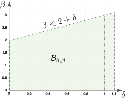
Figure 1: Region of parameters $\mathcal{B}_{\delta,\beta}$ (light green) in the plane $(\delta,\beta)$, for which there exists a homoclinic trajectory in system (4).

The eigenvalues and eigenvectors of the matrix of the linear part of (4) at the saddle $S_{0}$ have the following form:

$$\lambda^{\rm s}=-\alpha=-\delta\sqrt{1-s}, {\rm v}^{\rm s}=(0,\ 0,\ 1),$$ (23)

$$\lambda^{\rm ss}=\tfrac{1}{2}\big{(}-\sqrt{\lambda^{2}+4}-\lambda\big{)}=-\tfrac{1}{\sqrt{1-s}}, {\rm v}^{\rm ss}=\big{(}-\!\sqrt{1-s},\ 1,\ 0\big{)},$$

$$\lambda^{\rm u}=\tfrac{1}{2}\big{(}\sqrt{\lambda^{2}+4}-\lambda\big{)}=\sqrt{1-s}, {\rm v}^{\rm u}=\big{(}\tfrac{1}{\sqrt{1-s}},\ 1,\ 0\big{)},$$

where ${\rm v}^{\rm s}$, ${\rm v}^{\rm ss}$, ${\rm v}^{\rm u}$ are mutually perpendicular and the saddle value $\sigma_{0}=\lambda^{\rm u}+\lambda^{\rm s}=(1-\delta)\sqrt{1-s}\geq 0$ is zero if $\delta=1$ and positive if $\delta\in(0,1)$. The equilibrium $S_{0}$ has stable and unstable local invariant manifolds $W_{\rm loc}^{\rm s}$ и $W_{\rm loc}^{\rm u}$ of dimension $\dim W_{\rm loc}^{\rm s}=2$ and $\dim W_{\rm loc}^{\rm u}=1$, respectively, intersecting at $S_{0}$.

Remark 2.13.

The result of Corollary 2.12 for path (22) with $\beta\in(0,2)$ and $\delta=1$ was proved in Leonov [2015, 2016] and repeated in Ovsyannikov & Turaev [2017] taking into account transformation (7).

All the homoclinic bifurcations considered in Leonov [2012a, b, c, 2013a, 2013b, 2015, 2016] are described by the following two scenarios: either the change of attracting equilibria for separatrices of the saddle, or the merging of two stable limit cycles into one stable limit cycle. Here, using numerical simulations, we describe for $\delta<1$ several new homoclinic bifurcations.

3 Numerical analysis of stability/instability of homoclinic butterfly in the Lorentz-like system

Homoclinic bifurcation phenomena is related to the mathematical description of the transition to chaos know in literature as Shilnikov chaos. Numerical analysis and visualization of Shilnikov chaos is a difficult task, since it requires the study of unstable structures that are sensitive to errors in numerical methods.

In this article, to analyze the scenarios of homoclinic bifurcations and possible onset of chaotic behavior we perform a simple numerical scanning of the parameter region $\mathcal{B}_{\delta,\beta}=\{(\delta,\beta)\,\big{|}\,\delta\in(0,\,1.1],\,\beta\in(0,2+\delta)\}$ (see Fig. 1) and for a fixed pair $(\delta,\beta)\in\mathcal{B}_{\delta,\beta}$ we calculate the approximate interval $[\underline{s}\,,\overline{s}]\subset(0,1)$, such that for $s_{0}\in[\underline{s}\,,\overline{s}]$ there exist a homoclinic orbit. We select the grid of points $B_{\rm grid}\subset\mathcal{B}_{\delta,\beta}$ with the predefined step $\delta_{\rm grid}$ and for each point $(\delta_{\rm curr},\beta_{\rm curr})\in B_{\rm grid}$ we choose the partition $0<s_{\rm step}^{0}<2s_{\rm step}^{0}<3s_{\rm step}^{0}<\dots,(N-1)s_{\rm step}^{0}<1$ of the interval $(0,1)$ with step $s_{\rm step}^{0}=\tfrac{1}{N}$. For the system (4) with parameters $\delta_{\rm curr},\beta_{\rm curr},\lambda(s_{\rm curr}),\alpha(s_{\rm curr})$ we will simulate separatrix $(x_{\rm sepa}(t),\vartheta_{\rm sepa}(t),u_{\rm sepa}(t))$ of the saddle $S_{0}$ of the system (4) by integrating them numerically on the chosen time interval $t\in[0,T_{\rm trans}]$ using the implementation of the numerical procedure ode45 for solving differential equations in MATLAB.

To determine possible existence of limit sets (stable limit cycles and attractors) we will also numerically integrate trajectories $x_{\rm lim}(t),\vartheta_{\rm lim}(t),u_{\rm lim}(t)$ with initial data $\left(x_{\rm lim}(0),\vartheta_{\rm lim}(0),u_{\rm lim}(0)\right)=\left(x_{\rm sepa}(T_{\rm trans}),\vartheta_{\rm sepa}(T_{\rm trans}),u_{\rm sepa}(T_{\rm trans})\right)$ on the chosen interval $t\in[0,T_{\rm lim}]$. Resulting trajectories $(x_{\rm sepa}(t),\vartheta_{\rm sepa}(t),u_{\rm sepa}(t))$ and $(x_{\rm lim}(t),\vartheta_{\rm lim}(t),u_{\rm lim}(t))$ will be colored according to the color scale from blue to red, corresponding to the integration time interval (this will help us to determine the twisting / untwisting of the trajectory). Note that due to symmetry of the system (4) it is enough to integrate only one separatrix $\Gamma^{+}(t)=(x_{\rm sepa}(t),\vartheta_{\rm sepa}(t),u_{\rm sepa}(t))$ and the second one can be expressed as $\Gamma^{-}(t):=(-x_{\rm sepa}(t),-\vartheta_{\rm sepa}(t),u_{\rm sepa}(t))$. When equilibria $S_{\pm}$ are saddle-foci, we also simulate the separatrix of the $S_{+}$ in the described above manner.

In numerical integration of trajectories via ode45 we use the event handler ODE Event Location and handle the following events:

• separatrix $\Gamma^{+}(t)$ tends to infinity. For the values of parameter $s$ close to $0$ system (4) is not dissipative in the sense of Levinson, and the separatrix of the saddle $S_{0}$ will slowly untwist to ”infinity”. Therefore, the procedure will be terminated if the separatrix leaves the sphere with a big enough radius $R_{\rm inf}$.

• separatrix $\Gamma^{+}(t)$ tends to equilibrium $S_{+}$ (or $\Gamma^{-}(t)$ to $S_{-}$), towards which it was released. If for some $s=s_{\rm cr}$ the separatrix tends to nearest equilibrium state, then for $s>s_{\rm cr}$ there will be no other bifurcations. At this point it is possible to terminate the scanning by parameter $s$ and start modeling of the next pair $(\delta,\beta)$. To examine the attraction to the equilibrium state it was detected the event of falling into its small neighborhood of the radius $\varepsilon_{\rm eq}$.

If for a fixed pair $(\delta,\beta)$ during the scanning of the interval $(0,1)$ with the step $s_{\rm step}^{0}$ there are two consecutive values $\underline{s},\overline{s}\in(0,1)$ such that the behavior of the separatrices $\Gamma^{\pm}(t)$ changes as we go from the parameters $\lambda(\underline{s})$, $\alpha(\underline{s})$ to the parameters $\lambda(\overline{s})$, $\alpha(\overline{s})$, then the segment $[\underline{s}\,,\overline{s}]$ is also scanned with the $s_{\rm step}^{1}=0.1s_{\rm step}^{0}$. This gradual reduction in the partitioning step allows us to find the boundary values $\underline{s}$, $\overline{s}$ which specify a bifurcation with a certain accuracy $\overline{s}-\underline{s}>\varepsilon_{\rm threshold}$.

Values of the parameters of the numerical procedure for scanning the region $\mathcal{B}_{\delta,\beta}$. $\delta_{\rm grid}$ $s_{\rm step}^{0}$ $\varepsilon_{\rm threshold}$ $T_{\rm trans}$ $T_{\rm lim}$ $R_{\rm inf}$ $\varepsilon_{\rm eq}$ RelTol AbsTol $10^{-2}$ $10^{-3}$ $10^{-12}$ $4\cdot 10^{3}$ $10^{3}$ $100$ $10^{-1}$ $10^{-15}$ $10^{-15}$

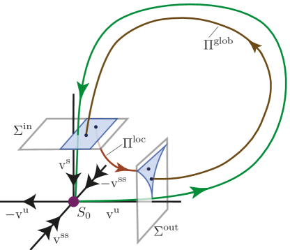
Figure 2: Poincaré sections $\Sigma^{\rm in}$ and $\Sigma^{\rm out}$ in the neighborhood of the saddle $S_{0}=(0,0,0)$ of the system (4).

After the described scanning of the region $\mathcal{B}_{\delta,\beta}$ for each grid point $(\delta,\beta)\in B_{\rm grid}$ the values $\underline{s},\overline{s}\in(0,1)$ are found numerically, such that the change of the parameter $s$ on the interval $[\underline{s}\,,\overline{s}]\subset(0,1)$ specifies a homoclinic bifurcation. Further, the type of homoclinic bifurcation was refined by numerical analysis of the behavior of the Poincaré map on the corresponding sections $\Sigma^{\rm in}$, $\Sigma^{\rm out}$, chosen in the neighborhood of the saddle $S_{0}$ (Fig. 2). The section $\Sigma^{\rm in}$ is chosen perpendicular to the vector ${\rm v^{s}}$ at a distance of $\varepsilon^{\rm in}$ from $S_{0}$, the section $\Sigma^{\rm out}$ – is perpendicular to the vector ${\rm v^{u}}$ and is located at a distance of $\varepsilon^{\rm out}$ from $S_{0}$. On the section $\Sigma^{\rm in}$ a rectangular grid of points $\Sigma^{\rm in}_{\rm grid}$ with sides collinear to the vectors ${\rm v^{u}}$ and ${\rm v^{ss}}$ is chosen. We match the color according to the color scale (from blue to red) to each row of grid points, starting with the row that lies at the intersection of $\Sigma^{\rm in}$ and the plane $\{{\rm v^{s}},{\rm v^{ss}}\}$, and paint the grid in this way (Fig. 3). Next, the evolution of the Poincare map $\Pi=\Pi^{\rm glob}\circ\Pi^{\rm loc}:\Sigma^{\rm in}\to\Sigma^{\rm in}$ of the given grid of points $\Sigma^{\rm in}_{\rm grid}$ is numerically studied. In our experiment, the maps $\Pi^{\rm loc}:\Sigma^{\rm in}\to\Sigma^{\rm out}$ and $\Pi^{\rm glob}:\Sigma^{\rm out}\to\Sigma^{\rm in}$ are simulated in MATLAB using numerical procedure ode45 and built-in event handler ODE Event Location to determine the moment of hitting on the corresponding section.

As a result of numerical experiments it was found that for a sufficiently small rectangle after the first Poincaré map its image falls inside its domain. Therefore, from the rectangular grid of points it is possible to cut out the middle part and to consider the half frame in the experiment. The size of the cutted-out part is chosen in such a way that the intersection point of the separatrix $\Gamma^{+}(t)$ released from the saddle $S_{0}$ with the section $\Sigma^{\rm in}$ belongs to it along with its small neighborhood. This approach allows us to avoid the simulation of the separatrices close to the homoclinic loop that requires calculations over large time intervals, since during the refinement of the bifurcation parameter, the separatrix becomes close to the homoclinic trajectory.

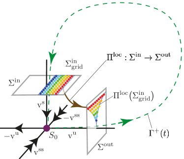
(a) $\Pi^{\rm loc}:\Sigma^{\rm in}\to\Sigma^{\rm out}$ maps rectangular grid of points $\Sigma^{\rm in}_{\rm grid}$ to a ”half bowtie” shape grid $\Pi^{\rm loc}\big{(}\Sigma^{\rm in}_{\rm grid}\big{)}$.

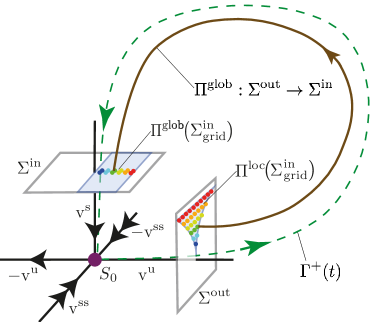
(b) $\Pi^{\rm glob}:\Sigma^{\rm out}\to\Sigma^{\rm in}$ shrinks $\Pi^{\rm loc}\big{(}\Sigma^{\rm in}_{\rm grid}\big{)}$ into a ”stick” shape grid $\Pi^{\rm glob}\big{(}\Sigma^{\rm in}_{\rm grid}\big{)}$.

Figure 3: Rectangular grid of points $\Sigma^{\rm in}_{\rm grid}$ and its image $\Pi^{\rm glob}\big{(}\Sigma^{\rm in}_{\rm grid}\big{)}$ on the Poincare section $\Sigma^{\rm in}$.

Numerical studies have shown that in the region covered by the given grid points, there are $4$ regions with different homoclinic bifurcations (Fig. 4). In the green region marked with ($\circ$) before bifurcation separatrices $\Gamma^{\pm}(t)$ were attracted to the opposite equilibria $S_{\mp}$ and after bifurcation – to the nearest ones, i.e. to $S_{\pm}$. In this case, during the inverse bifurcation (i.e. while moving in the direction from $s=1$ to $s=0$), two unstable limit cycles are born from the homoclinic butterfly. This scenario corresponds to the case of the homoclinic bifurcation in classical Lorenz system Lorenz [1963] with parameters $\sigma=10$, $b=8/3$, $r\in[13.9265574075,13.9265574076]$ (see e.g. Shilnikov et al. [2001]).

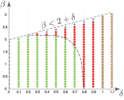
Figure 4: Different types of homoclinic bifurcations in the system (4).

In the orange region marked with ($\times$) during the bifurcation, one large stable ”eight”-type limit cycle splits into two stable limit cycles around $S_{\pm}$. Numerical analysis of the separatrices behavior for all $\beta\in(0,2+\delta)$ within the chosen partition and the dynamics analysis of the grid points $\Sigma^{\rm in}_{\rm grid}$ on the Poincaré section $\Sigma^{\rm in}$ under the successive action of Poincaré map $\Pi:\Sigma^{\rm in}\to\Sigma^{\rm in}$ give us a reason to state that there is no chaotic dynamics in the vicinity of the homoclinic bifurcation in the case of zero and negative saddle values.

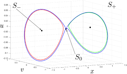
(a) $\text{\text@underline{s}}=0.060131460578$

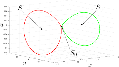
(b) $\overline{s}=0.060131460581$

Figure 5: Homoclinic bifurcation for $\delta=0.9$, $\beta=0.2$.

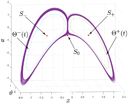
(a) $\text{\text@underline{s}}^{\prime}=0.7979407438278198$

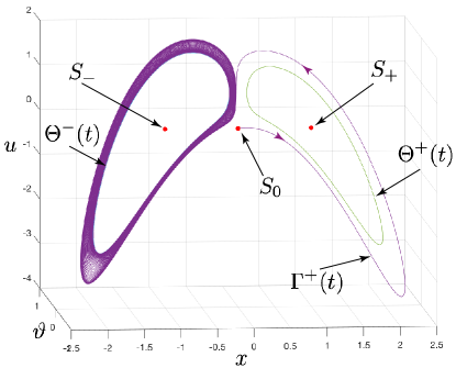
(b) $\text{\text@underline{s}}\in{[0.7979407447814941,0.8059291805341841]}$

Figure 6: Behavior of separatrix $\Gamma^{+}(t)$ of saddle $S_{0}$ and separatrices of saddle-foci $S_{\pm}$ before homoclinic bifurcation for $\delta=0.5$, $\beta=2.2$. Homoclinic bifurcation occurs on the interval $s\in[\underline{s},\overline{s}]$, where $\overline{s}=0.8059291805416346$.

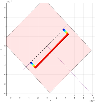
(a) $i=0$

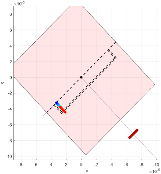
(b) $i=1$

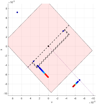
(c) $i=25$

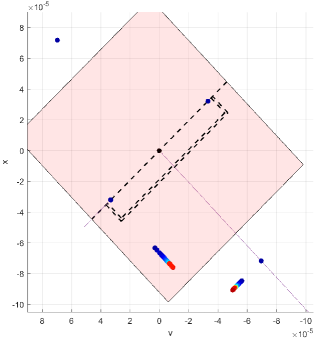
(d) $i=50$

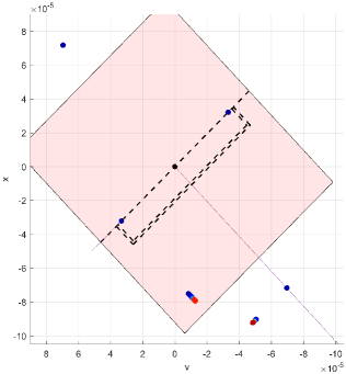
(e) $i=75$

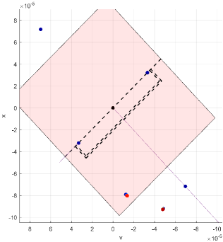
(f) $i=100$

Figure 9: Dynamics of the half-frame of points $\Sigma^{\rm in}_{\rm grid}$ on the section $\Sigma^{\rm in}$ under repeated applications of the Poincaré map $\Pi^{i}:\Sigma^{\rm in}\to\Sigma^{\rm in}$, $i=1,2,\dots$, for $\delta=0.9$, $\beta=0.2$, $\text{\text@underline{s}}=0.060131460578$ (before bifurcation).

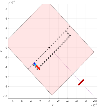
(b) $i=1$

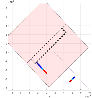
(c) $i=25$

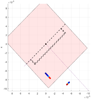
(d) $i=50$

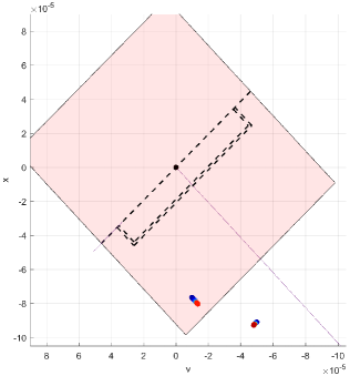
(e) $i=75$

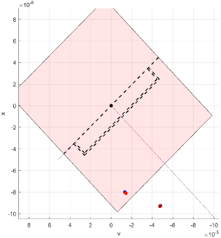
(f) $i=100$

Figure 10: Dynamics of the half-frame of points $\Sigma^{\rm in}_{\rm grid}$ on the section $\Sigma^{\rm in}$ under repeated applications of the Poincaré map $\Pi^{i}:\Sigma^{\rm in}\to\Sigma^{\rm in}$, $i=1,2,\dots$, for $\delta=0.9$, $\beta=0.2$, $\overline{s}=0.060131460581$ (after bifurcation).

Also, two new scenarios of homoclinic bifurcation were found. In the red area marked with ($\bullet$), depending on values of parameters $\delta$, $\beta$, two symmetric limit cycles $\Theta^{\pm}$ around $S_{\pm}$ coexist with either one stable ”eight”-type limit cycle, or a strange attractor which attract the separatrices $\Gamma^{\pm}(t)$. Then this attractor (periodic or strange) loses stability and separatrices $\Gamma^{\pm}(t)$ are attracted to the opposite limit cycles $\Theta^{\mp}$. After the bifurcation the separatrices $\Gamma^{\pm}(t)$ are attracted to the nearest limit cycles $\Theta^{\pm}$. As in the case of Lorenz system, in this case during the inverse bifurcation, two unstable limit cycles are born from the homoclinic butterfly, but here they separetes two stable cycles $\Theta^{\pm}$. For example, for parameter values $\delta=0.9$, $\beta=0.2$, the dynamics of separatrices in the phase space is shown in Fig. 5 and the dynamics of the grid of points $\Sigma^{\rm in}_{\rm grid}$ before and after bifurcation is presented in Fig. 9 and Fig. 10), respectively. For parameter values $\delta=0.5$, $\beta=2.2$ the case of coexistence of two symmetric limit cycles $\Theta^{\pm}$ around $S_{\pm}$ with a strange attractor defined by the separatrix $\Gamma^{+}(t)$ is presented in Fig. 6. Note that here one could consider two types of vicinities of the bifurcation point in the parameter space: $[\underline{s},\overline{s}]$ and $[\underline{s}^{\prime},\overline{s}]$, where $[\underline{s},\overline{s}]\subset[\underline{s}^{\prime},\overline{s}]$. In the vicinity $[\underline{s},\overline{s}]$ a simple bifurcation is observed in which, as described just above, there is a change in attracting limit cycles $\Theta^{\pm}$ for the separatrices $\Gamma^{\pm}(t)$ of the saddle $S_{0}$. At the same time, on the interval $[\underline{s}^{\prime},\underline{s})$ the chaotic behavior of the separatrices $\Gamma^{\pm}(t)$ can be observed, which can make one to think that the homoclinic bifurcation is embedded in the strange attractor.

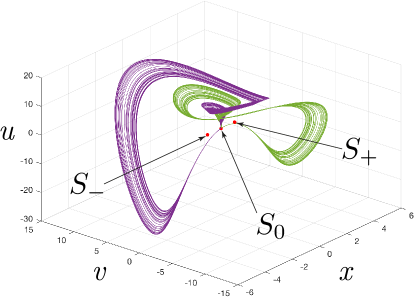
(a) $\overline{s}=0.7957...$

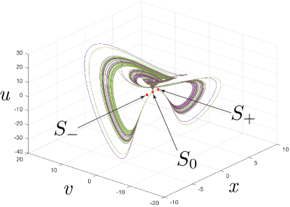
(b) $\text{\text@underline{s}}=0.7955...$

Figure 7: Homoclinic bifurcation of the two merging attractors at $\delta=0.9$, $\beta=2.899$.

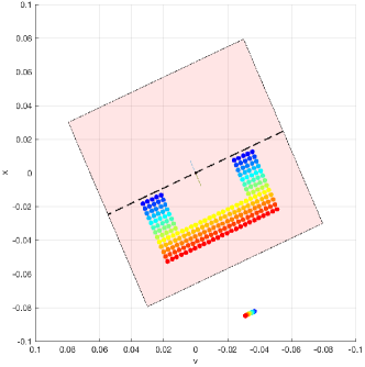
(a) $i=0$

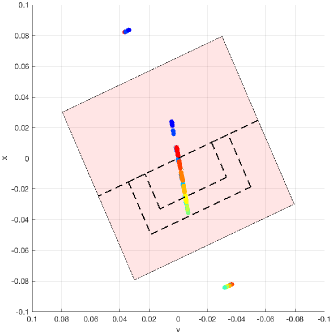
(b) $i=1$

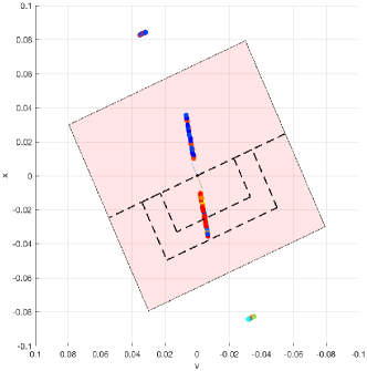
(c) $i=25$

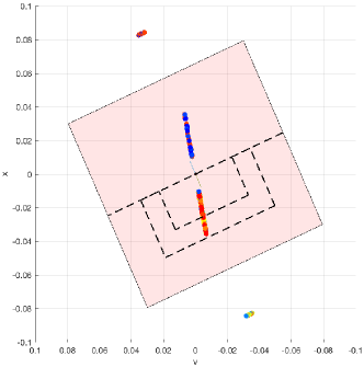
(d) $i=50$

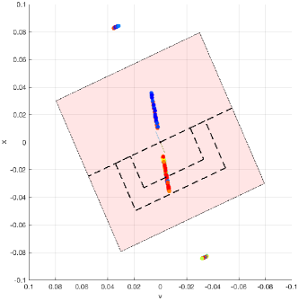
(e) $i=75$

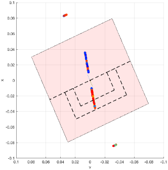
(f) $i=100$

Figure 11: Dynamics of the half-frame of points $\Sigma^{\rm in}_{\rm grid}$ on the section $\Sigma^{\rm in}$ under repeated applications of the Poincaré map $\Pi^{i}:\Sigma^{\rm in}\to\Sigma^{\rm in}$, $i=1,2,\dots$, for $\delta=0.9$, $\beta=2.899$, $\text{\text@underline{s}}=0.7955$ (before bifurcation).

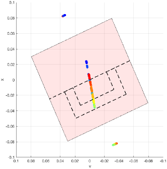
(b) $i=1$

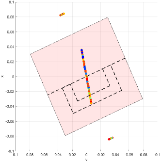
(c) $i=25$

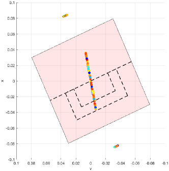
(d) $i=50$

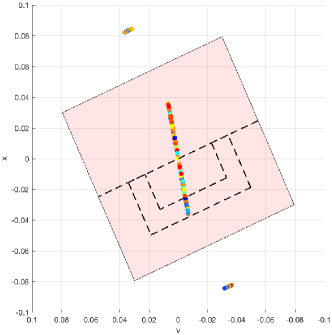
(e) $i=75$

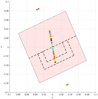
(f) $i=100$

Figure 12: Dynamics of the half-frame of points $\Sigma^{\rm in}_{\rm grid}$ on the section $\Sigma^{\rm in}$ under repeated applications of the Poincaré map $\Pi^{i}:\Sigma^{\rm in}\to\Sigma^{\rm in}$, $i=1,2,\dots$, for $\delta=0.9$, $\beta=2.899$, $\overline{s}=0.7958$ (after bifurcation).

In the blue region marked with ($\ast$) when an unstable homoclinic trajectory occurs, one strange attractor split into two (or, if we track the change in the parameter $s$ from $1$ to $0$, then we can say that two strange attractors merge into one strange attractor). For example, for parameter values $\delta=0.9$, $\beta=2.899$, the dynamics of separatrices in the phase space is shown in Fig. 7 and the dynamics of the grid of points $\Sigma^{\rm in}_{\rm grid}$ before and after bifurcation is presented in Fig. 11 and Fig. 12), respectively.

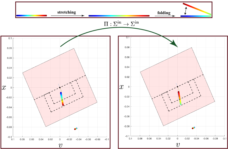
Figure 8: Behavior of the Poincaré map $\Pi:\Sigma^{\rm in}\to\Sigma^{\rm in}$ in the case of two splitting attractors of system (4) with $\delta=0.9$, $\beta=2.899$.

For numerical verification of the behavior of the Poincaré map $\Pi:\Sigma^{\rm in}\to\Sigma^{\rm in}$ for the case of splitting attractors we perform the following test. Consider the grid of points $\Sigma^{\rm attr}_{\rm grid}$ corresponding to the intersection between one of the attractors and the Poincaré section $\Sigma^{\rm in}$ and color it according to the scale (from blue to red). We save the coordinates of grid points assuming that approximately this grid represents the line segment. Next, we calculate the image of $\Sigma^{\rm attr}_{\rm grid}$ under the action of the Poincaré and after that for each point ${\rm x}_{0}\in\Sigma^{\rm attr}_{\rm grid}$ we compare its coordinate with the coordinate of $\Pi({\rm x}_{0})$. As a result of this experiment, we have obtained that, under the indicated assumptions, the Poincaré map behaves approximately the same way as the know one-dimensional tent map with parameter $\approx 2$ (Fig. 8). Using special methods for finite-time Lyapunov exponents and finite-time Lyapunov dimension estimations (see e.g. Leonov et al. [2015c, b, 2016]; Kuznetsov et al. [2018]), we calculate the corresponding values of the largest finite-time Lyapunov exponent, ${\rm LE}_{1}(t_{\rm end}{\rm x}_{0})=0.0316>0$, and local finite-time Lyapunov dimension, ${\rm LD}(t_{\rm end},{\rm x}_{0})=2.0131$ for one of the attractors along the trajectory with initial data ${\rm x}_{0}=(-0.0479075467563750,8.41428910156156,13.7220943173008)$ and time interval $[0,t_{\rm end}]$, $t_{\rm end}=1000$. These numerical experiments give us a reason to think that the considered attractor (and the symmetric one) is strange.

Numerical simulations of separatrices outside the region $\mathcal{B}_{\delta,\beta}$ (i.e. for the case $\beta>2+\delta$) show that system (4) in this region is not dissipative in the sense of Levinson and separatrices tend to infinity. Thus, numerically we obtain that outside the region $\mathcal{B}_{\delta,\beta}$ there are no homoclinic bifurcations. Later on we are going to prove it analytically.

This article is the beginning of a study of this type of homoclinic bifurcation. Further studies in this direction may require the introduction of the new mathematical concepts into consideration, and the development of the new numerical methods with a high performance computing. Also, the authors plan to take into consideration recently developed new reliable numerical methods for studying trajectories of the Lorenz-like systems (see e.g. Tucker [1999]; Liao & Wang [2014]; Lozi & Pchelintsev [2015]; Kehlet & Logg [2017]) and the existing approaches for the analysis of homoclinic bifurcations (see e.g. Wiggins [1988]; Champneys et al. [1996]; Doedel & et. al [2007]; Homburg & Sandstede [2010]).

4 Conclusion

In papers Leonov [2012a, 2013b]; Leonov et al. [2015c], effective analytical and analytical-numerical methods for studying homoclinic bifurcations and Shilnikov scenarios of system’s behavior in its vicinity were developed. However, subsequent studies Leonov & Mokaev [2018a, b]; Leonov [2018] have shown the practical difficulties of the numerical implementation of these methods related to the calculations with finite accuracy and round-off errors. In this paper we have tried to overcome these difficulties as much as possible while remaining within the framework of standard calculations in Matlab. Thus, in this paper the following results were obtained. We prove analytically the existence of homoclinic orbit to a saddle zero equilibrium in the Lorenz-like system (4) and perform a numerical scanning of the corresponding parameter region where the homoclinic bifurcations occur. As a result, numerical confirmation of possible Shilnikov scenarios and new scenarios of homoclinic bifurcations in system (4) were found numerically, e.g., the unstable homoclinic bifurcation of two merging strange attractors.

Numerical results on the merging attractors bifurcation emphasize the fact that when studying homoclinic bifurcations it is not sufficient to investigate the local behavior of the system in a neighborhood of a saddle equilibrium. The effects of stretching and compression in the vicinity of the homoclinic trajectory could be influenced greatly by the global behavior of the system outside the saddle.

5 Acknowledgment

This publication was supported by the grant of the President of Russian Federation for the Leading Scientific Schools of Russia [NSh-2858.2018.1] (namely, in Section 2: analytical proof of the existence of homoclinic orbits in system (4), and in Section 3: initial numerical study of the region $\mathcal{B}_{\delta,\beta}$ of existence of homoclinic orbits), and by the grant of the Russian Science Foundation [project 14-21-00041] (namely, in Section 3: clarification of homoclinic bifurcation scenarios using standard Matlab framework, numerical confirmation of possible Shilnikov scenarios, and numerical analysis of chaotic attractors arising from the merge bifurcation).

(a) $i=0$

(a) $i=0$

References

- Afraimovich et al. [2014] Afraimovich, V. S., Gonchenko, S. V., Lerman, L. M., Shilnikov, A. L. & Turaev, D. V. [2014] “Scientific heritage of LP Shilnikov,” Regular and Chaotic Dynamics 19, 435–460.
- Argoul et al. [1987] Argoul, F., Arneodo, A. & Richetti, P. [1987] “Experimental evidence for homoclinic chaos in the belousov-zhabotinskii reaction,” Physics Letters A 120, 269–275.
- Champneys [1998] Champneys, A. [1998] “Homoclinic orbits in reversible systems and their applications in mechanics, fluids and optics,” Physica D: Nonlinear Phenomena 112, 158–186.
- Champneys et al. [1996] Champneys, A., Kuznetsov, Y. & Sandstede, B. [1996] “A numerical toolbox for homoclinic bifurcation analysis,” International Journal of Bifurcation and Chaos 6, 867–888.
- Chen et al. [2017] Chen, G., Kuznetsov, N., Leonov, G. & Mokaev, T. [2017] “Hidden attractors on one path: Glukhovsky-Dolzhansky, Lorenz, and Rabinovich systems,” International Journal of Bifurcation and Chaos 27, art. num. 1750115.
- Chen & Ueta [1999] Chen, G. & Ueta, T. [1999] “Yet another chaotic attractor,” International Journal of Bifurcation and Chaos 9, 1465–1466.
- Doedel & et. al [2007] Doedel, E. & et. al [2007] “AUTO-07P: Continuation and bifurcation software for ordinary differential equations,” URL http://www.dam.brown.edu/people/sandsted/auto/auto07p.pdf.
- Grebogi et al. [1983] Grebogi, C., Ott, E. & Yorke, J. [1983] “Fractal basin boundaries, long-lived chaotic transients, and unstable-unstable pair bifurcation,” Physical Review Letters 50, 935–938.
- Homburg & Sandstede [2010] Homburg, A. J. & Sandstede, B. [2010] “Homoclinic and heteroclinic bifurcations in vector fields,” Handbook of dynamical systems 3, 379–524.
- Kehlet & Logg [2017] Kehlet, B. & Logg, A. [2017] “A posteriori error analysis of round-off errors in the numerical solution of ordinary differential equations,” Numerical Algorithms 76, 191–210.
- Kuznetsov et al. [2018] Kuznetsov, N., Leonov, G., Mokaev, T., Prasad, A. & Shrimali, M. [2018] “Finite-time Lyapunov dimension and hidden attractor of the Rabinovich system,” Nonlinear Dynamics 92, 267–285, 10.1007/s11071-018-4054-z.
- Kuznetsov et al. [1992] Kuznetsov, Y., Muratori, S. & Rinaldi, S. [1992] “Bifurcations and chaos in a periodic predator-prey model,” International Journal of Bifurcation and Chaos 2, 117–128.
- Lai & Tel [2011] Lai, Y. & Tel, T. [2011] Transient Chaos: Complex Dynamics on Finite Time Scales (Springer, New York).
- Leonov [2012a] Leonov, G. [2012a] “General existence conditions of homoclinic trajectories in dissipative systems. Lorenz, Shimizu-Morioka, Lu and Chen systems,” Physics Letters A 376, 3045–3050.
- Leonov [2013a] Leonov, G. [2013a] “Criteria for the existence of homoclinic orbits of systems Lu and Chen,” Doklady Mathematics 87, 220–223.
- Leonov [2013b] Leonov, G. [2013b] “Shilnikov chaos in Lorenz-like systems,” International Journal of Bifurcation and Chaos 23, 10.1142/S0218127413500582, art. num. 1350058.
- Leonov [2014a] Leonov, G. [2014a] “Fishing principle for homoclinic and heteroclinic trajectories,” Nonlinear Dynamics 78, 2751–2758.
- Leonov [2014b] Leonov, G. [2014b] “Rössler systems: estimates for the dimension of attractors and homoclinic orbits,” Doklady Mathematics 89, 369–371.
- Leonov [2015] Leonov, G. [2015] “Cascade of bifurcations in Lorenz-like systems: Birth of a strange attractor, blue sky catastrophe bifurcation, and nine homoclinic bifurcations,” Doklady Mathematics 92, 563–567.
- Leonov [2016] Leonov, G. [2016] “Necessary and sufficient conditions of the existence of homoclinic trajectories and cascade of bifurcations in Lorenz-like systems: birth of strange attractor and 9 homoclinic bifurcations,” Nonlinear Dynamics 84, 1055–1062.
- Leonov [2018] Leonov, G. [2018] “Lyapunov functions in the global analysis of chaotic systems,” Ukrainian Mathematical Journal 70, 42–66.
- Leonov et al. [2015a] Leonov, G., Alexeeva, T. & Kuznetsov, N. [2015a] “Analytic exact upper bound for the Lyapunov dimension of the Shimizu-Morioka system,” Entropy 17, 5101–5116, 10.3390/e17075101.
- Leonov et al. [2017] Leonov, G., Andrievskiy, B. & Mokaev, R. [2017] “Asymptotic behavior of solutions of Lorenz-like systems: Analytical results and computer error structures,” Vestnik St. Petersburg University. Mathematics 50, 15–23.
- Leonov & Kuznetsov [2015] Leonov, G. & Kuznetsov, N. [2015] “On differences and similarities in the analysis of Lorenz, Chen, and Lu systems,” Applied Mathematics and Computation 256, 334–343, 10.1016/j.amc.2014.12.132.
- Leonov et al. [2016] Leonov, G., Kuznetsov, N., Korzhemanova, N. & Kusakin, D. [2016] “Lyapunov dimension formula for the global attractor of the Lorenz system,” Communications in Nonlinear Science and Numerical Simulation 41, 84–103, 10.1016/j.cnsns.2016.04.032.
- Leonov et al. [2015b] Leonov, G., Kuznetsov, N. & Mokaev, T. [2015b] “Hidden attractor and homoclinic orbit in Lorenz-like system describing convective fluid motion in rotating cavity,” Communications in Nonlinear Science and Numerical Simulation 28, 166–174, 10.1016/j.cnsns.2015.04.007.
- Leonov et al. [2015c] Leonov, G., Kuznetsov, N. & Mokaev, T. [2015c] “Homoclinic orbits, and self-excited and hidden attractors in a Lorenz-like system describing convective fluid motion,” The European Physical Journal Special Topics 224, 1421–1458, 10.1140/epjst/e2015-02470-3.
- Leonov & Mokaev [2018a] Leonov, G. & Mokaev, R. [2018a] “Homoclinic bifurcations of the merging strange attractors in the Lorenz-like system,” arXiv preprint arXiv:1802.07694v1 .
- Leonov & Mokaev [2018b] Leonov, G. & Mokaev, R. [2018b] “Numerical simulations of the Lorenz-like system: Asymptotic behavior of solutions, chaos and homoclinic bifurcations,” Abstracts of the International Scientific Conference on Mechanics ”The Eight Polyakhov’s Reading”, p. 264.
- Leonov [2012b] Leonov, G. A. [2012b] “Criteria for the existence of homoclinic orbits of systems Lu and Chen,” Doklady Mathematics 87, 220–223.
- Leonov [2012c] Leonov, G. A. [2012c] “Tricomi problem for Shimizu-Morioka dynamical system,” Doklady Mathematics 86, 850–853.
- Liao & Wang [2014] Liao, S. & Wang, P. [2014] “On the mathematically reliable long-term simulation of chaotic solutions of Lorenz equation in the interval [0,10000],” Science China Physics, Mechanics and Astronomy 57, 330–335.
- Lorenz [1963] Lorenz, E. [1963] “Deterministic nonperiodic flow,” J. Atmos. Sci. 20, 130–141.
- Lozi & Pchelintsev [2015] Lozi, R. & Pchelintsev, A. [2015] “A new reliable numerical method for computing chaotic solutions of dynamical systems: the Chen attractor case,” International Journal of Bifurcation and Chaos 25, 1550187.
- Lu & Chen [2002] Lu, J. & Chen, G. [2002] “A new chaotic attractor coined,” Int. J. Bifurcation and Chaos 12, 1789–1812.
- Neimark & Landa [1992] Neimark, Y. I. & Landa, P. S. [1992] Stochastic and Chaotic Oscillations (Kluwer Academic Publishers, Dordrecht, The Netherlands).
- Oraevsky [1981] Oraevsky, A. N. [1981] “Masers, lasers, and strange attractors,” Quantum Electronics 11, 71–78.
- Ovsyannikov & Turaev [2017] Ovsyannikov, I. & Turaev, D. [2017] “Analytic proof of the existence of the Lorenz attractor in the extended Lorenz model,” Nonlinearity 30, 115.
- Poincare [1892, 1893, 1899] Poincare, H. [1892, 1893, 1899] Les methodes nouvelles de la mecanique celeste. Vol. 1-3 (Gauthiers-Villars, Paris), [English transl. edited by D. Goroff: American Institute of Physics, NY, 1993].
- Rubenfeld & Siegmann [1977] Rubenfeld, L. A. & Siegmann, W. L. [1977] “Nonlinear dynamic theory for a double-diffusive convection model,” SIAM Journal on Applied Mathematics 32, 871–894.
- Shilnikov et al. [2001] Shilnikov, L., Shilnikov, A., Turaev, D. & Chua, L. [2001] Methods of Qualitative Theory in Nonlinear Dynamics: Part 2 (World Scientific).
- Shilnikov et al. [1998] Shilnikov, L. P., Shilnikov, A. L., Turaev, D. V. & Chua, L. [1998] Methods of Qualitative Theory in Nonlinear Dynamics: Part 1 (World Scientific).
- Shimizu & Morioka [1980] Shimizu, T. & Morioka, N. [1980] “On the bifurcation of a symmetric limit cycle to an asymmetric one in a simple model,” Physics Letters A 76, 201 – 204.
- Tel & Gruiz [2006] Tel, T. & Gruiz, M. [2006] Chaotic dynamics: An introduction based on classical mechanics (Cambridge University Press).
- Tigan & Opris [2008] Tigan, G. & Opris, D. [2008] “Analysis of a 3D chaotic system,” Chaos, Solitons & Fractals 36, 1315–1319.
- Tricomi [1933] Tricomi, F. [1933] “Integrazione di unequazione differenziale presentatasi in elettrotechnica,” Annali della R. Shcuola Normale Superiore di Pisa 2, 1–20.
- Tucker [1999] Tucker, W. [1999] “The Lorenz attractor exists,” Comptes Rendus de l’Academie des Sciences - Series I - Mathematics 328, 1197 – 1202.
- Wiggins [1988] Wiggins, S. [1988] Global bifurcations and chaos: analytical methods, Vol. 73 (Springer-Verlag).
- Yang & Chen [2008] Yang, Q. & Chen, G. [2008] “A chaotic system with one saddle and two stable node-foci,” International Journal of Bifurcation and Chaos 18, 1393–1414, 10.1142/S0218127408021063.