Stellar population of the superbubble N 206 in the LMC

Abstract

Context. Clusters or associations of early-type stars are often associated with a ‘superbubble’ of hot gas. The formation of such superbubbles is caused by the feedback from massive stars. The complex N 206 in the Large Magellanic Cloud exhibits a superbubble and a rich massive star population.

Aims. Our goal is to perform quantitative spectral analyses of all massive stars associated with the N 206 superbubble in order to determine their stellar and wind parameters. We compare the superbubble energy budget to the stellar energy input and discuss the star formation history of the region.

Methods. We observed the massive stars in the N 206 complex using the multi-object spectrograph FLAMES at ESO’s Very Large Telescope (VLT). Available ultra-violet (UV) spectra from archives are also used. The spectral analysis is performed with Potsdam Wolf-Rayet (PoWR) model atmospheres by reproducing the observations with the synthetic spectra.

Results. We present the stellar and wind parameters of the OB stars and the two Wolf-Rayet (WR) binaries in the N 206 complex. Twelve percent of the sample show Oe/Be type emission lines, although most of them appear to rotate far below critical. We found eight runaway stars based on their radial velocity. The wind-momentum luminosity relation of our OB sample is consistent with the expectations. The Hertzsprung-Russell diagram (HRD) of the OB stars reveals a large age spread ($1-30$ Myr), suggesting different episodes of star formation in the complex. The youngest stars are concentrated in the inner part of the complex, while the older OB stars are scattered over outer regions. We derived the present day mass function for the entire N 206 complex as well as for the cluster NGC 2018. The total ionizing photon flux produced by all massive stars in the N 206 complex is $Q_{0}\approx 5\times 10^{50}\,\rm{s^{-1}}$, and the mechanical luminosity of their stellar winds amounts to $L_{\rm{mec}}=1.7\times 10^{38}\,\rm{erg\,s^{-1}}$. Three very massive Of stars are found to dominate the feedback among 164 OB stars in the sample. The two WR winds alone release about as much mechanical luminosity as the whole OB star sample. The cumulative mechanical feedback from all massive stellar winds is comparable to the combined mechanical energy of the supernova explosions that likely occurred in the complex. Accounting also for the WR wind and supernovae, the mechanical input over the last five Myr is $\approx 2.3\times 10^{52}\,\rm{erg}$.

Conclusions. The N206 complex in the LMC has undergone star formation episodes since more than 30 Myr ago. From the spectral analyses of its massive star population, we derive a current star formation rate of $2.2\times 10^{-3}M_{\odot}\,\mathrm{yr}^{-1}$. From the combined input of mechanical energy from all stellar winds, only a minor fraction is emitted in the form of X-rays. The corresponding input accumulated over a long time also exceeds the current energy content of the complex by more than a factor of five. The morphology of the complex suggests a leakage of hot gas from the superbubble.

1 Introduction

Understanding the feedback of stars on their environment is one of the key problems in star and galaxy formation. Massive stars are the main feedback agents, altering the surrounding environment on local, global, and cosmic scales. They dynamically shape the interstellar medium (ISM) around them on timescales of a few Myr. With their winds, ionizing radiation, and supernova explosions, ensembles of massive stars cause the largest structures of the ISM such as giant or multiple H ii regions, superbubbles, and supergiant shells.

The interaction via winds and ionizing radiation of a single massive star with its surroundings is usually referred to as an interstellar bubble (Weaver et al. 1977). A massive star first forms an H ii region around itself through its strong ionizing radiation field, and its stellar wind interacts with this ionized gas. The supersonic stellar wind (typically 2000 km/s) drives a shock into the ambient medium, while the reverse shock decelerates the wind material, and the kinetic energy of the shocked stellar wind becomes thermal energy, leading to a hot ($T>10^{6}$ K), very low density bubble that emits soft X-rays. In a cluster, these hot bubbles around stars can interact with each other and form a superbubble (Tenorio-Tagle & Bodenheimer 1988; Oey et al. 2001; Chu 2008). Superbubbles are observed around many young massive star clusters with sizes of hundreds of parsecs (Tenorio-Tagle & Bodenheimer 1988; Sasaki et al. 2011).

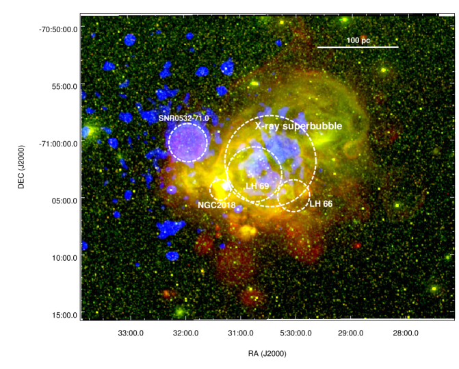
Figure 1: Location of the X-ray superbubble, SNR B0532-71.0, cluster NGC 2018, and OB associations LH 66 and LH 69 in the N 206 complex. The three-color composite image (H$\alpha$ (red) + [O iii] (green) + X-ray (blue)) shown in the background is from the Magellanic Cloud Emission-Line Survey (MCELS, Smith et al. 2005) and XMM-Newton ($0.3-1$ keV).

In a series of papers, we study the superbubble associated with the giant H ii region N 206 in the Large Magellanic Cloud (LMC). The LMC is one of the closest galaxies to the Milky Way with a distance modulus of only DM = 18.5 mag (Madore & Freedman 1998), allowing for detailed spectroscopy of its bright stars. Another advantage of the LMC is the marginal foreground reddening along the line of sight (Subramaniam 2005; Haschke et al. 2011). The LMC is chemically less evolved than the Milky Way with a metallicity around $Z=0.5\,Z_{\odot}$ (Rolleston et al. 2002). This allows us to study how stellar feedback works at sub-solar metallicity.

Our target of study is the high-mass star-forming complex N 206 (alias: Henize 206, LHA 120-N 206, and DEM L 221) in the outskirts of the LMC that surrounds the star forming cluster NGC 2018 (LHA 120-N 206A). This H ii region was first cataloged in an H$\alpha$ objective prism survey by Karl Henize in 1956 (Henize 1956). The N 206 complex also harbors a supernova remnant (SNR) B0532-71.0 (Mathewson & Clarke 1973; Williams et al. 2005) in the eastern part. The N 206 complex has been studied in multiwavelengths by various authors. Dunne et al. (2001) reported the expansion velocity of the H$\alpha$ shell to be $\sim$30 km/s. Since the superbubble has expanded to a diameter of $\sim$112 pc, this suggests an age of $\sim$2 Myr. More than one hundred young stellar object (YSO) candidates were identified in this region using infrared data from Spitzer, and a star formation rate (SFR) of $0.25\times 10^{-2}\,M_{\odot}$ yr^-1 has been estimated (Carlson et al. 2012; Romita et al. 2010; Gorjian et al. 2004).

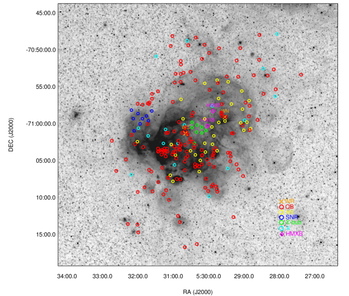
Figure 2: Position of all VLT-FLAMES MEDUSA fibers on the N 206 complex, including the OB-type stars (red circle), WR (orange cross), H ii region (yellow circle), SNR (blue circle), X-ray superbubble (green circle), A-type stars (cyan circle), and candidate HMXBs (magenta diamond). The background image shown is H$\alpha$ emission from the Magellanic Cloud Emission-Line Survey (MCELS, Smith et al. 2005).

The central part of the region is filled with hot gas and has been detected in X-rays. This X-ray superbubble is excited by the winds of the massive stars in the young cluster NGC 2018 as well as the LH 66 and LH 69 OB associations (Lucke & Hodge 1970) (see Sect. 2 for more details of the structure of the region). Dunne et al. (2001) concluded that current star formation is taking place around the X-ray superbubble. A detailed study of the complex in X-rays using the XMM-Newton telescope was published by Kavanagh et al. (2012). They compared the thermal energy stored in the X-ray emitting gas of the superbubble and the mechanical input supplied by the stellar population. Moreover, they found that the pressure of the hot gas drives the expansion of the shell into the surrounding H i cloud. They estimated the overall mass and thermal energy content of the superbubble and blowout region as 741$\pm$85 M_⊙ and (3.5$\pm 1.3)\times 10^{51}$ erg from soft diffuse X-ray emission and H$\alpha$ emission. However, this study was lacking information about the energetics of the complete massive star population in this region.

For a better understanding of a star-forming complex, we need to probe its stellar content in detail. In terms of brightness and youth, OB stars are excellent tracers of star formation. Their feedback effects can also lead to sequential star formation in these regions (Gouliermis et al. 2008; Smith et al. 2010; Chen et al. 2007). Therefore, the quantitative spectroscopy of OB star populations associated with superbubbles is essential to provide constraints on their fundamental parameters. By analyzing the massive star content of N 206 using sophisticated model atmospheres, we can derive the stellar and wind parameters of the individual stars as well as their ionizing fluxes. This, in turn, will enable us to compare the energy budget of the cluster with the energy stored in the X-ray superbubble.

This is the second paper in the series that presents the spectroscopic analysis of the entire massive star population in the N 206 superbubble. In the first paper of the series, we focused on the Of-type stars (Ramachandran et al. 2018, hereafter Paper I). Here we present the spectroscopic analysis of all remaining massive stars in this region, and finally discuss the total stellar feedback and the energy budget of the superbubble.

Section 2 briefly describes the spatial structure of the complex. The spectroscopic observations and spectral classifications are presented in Sections 3 and 4. In Sect. 5 and Sect. 6, we quantitatively analyze the OB star spectra and the Wolf-Rayet (WR) binary spectra using Potsdam Wolf-Rayet (PoWR) atmosphere models. In Sect. 7, the results are presented and discussed. The final Sect. 8 provides a summary and general conclusions. The Appendices encompass tables with all stellar parameters and figures with the spectral fits of the analyzed stars.

2 Spatial structure of the N 206 complex

A color composite image of the N 206 superbubble in H$\alpha$ (red), O iii (green), and in $0.3-1$ keV X-ray (blue) is shown in Fig. 1. The H$\alpha$ emission basically traces the H ii region in the complex. The entire structure is distributed over an approximately circular region with a diameter of $\approx$32$\arcmin$, corresponding to 465 pc. The complex encompasses an X-ray superbubble, a supernova remnant (SNR), the young cluster NGC 2018, and the OB associations LH 66 and LH 69.

The superbubble has been studied by many authors using Chandra and XMM-Newton data. It has a circular shell of diameter $\approx 8\arcmin$ (120 pc). The brightest H$\alpha$ emission originates in the eastern and southern sides of the bubble (Dunne et al. 2001). According to Dunne et al. (2001), the brightest X-ray emitting region of the superbubble is confined by an H$\alpha$ structure. A soft diffuse X-ray emission is detected across both the remnant and the superbubble. Kavanagh et al. (2012) noticed that no X-ray emission is detected from the major part of the superbubble region, and the hot X-ray emitting gas is distributed in a non-uniform manner.

The X-ray superbubble is surrounded by and overlaps with the young cluster NGC 2018 and the OB associations LH 66 and LH 69. This region contains 41 OB stars including four Of-type stars (N206-FS 111, 131, 162, and 178 analyzed in Paper I). Two WR binaries are present in the N 206 complex. The WC binary is located nearly at the center and the WN binary near the edge of the X-ray superbubble. The OB associations LH 66 and LH 69 occupy an approximately circular region of 3.3$\arcmin$ and 4.8$\arcmin$ in diameter. They harbor 12 and 29 OB stars, respectively. The entire LH 69 OB association is located within the boundaries of the X-ray superbubble region. The young cluster NGC 2018 is very bright in H$\alpha$. The emission spans over a region of $\approx 2\arcmin$ in diameter. This cluster encompasses 14 OB stars, mostly young O stars including three Of-type stars (N206-FS 180, 187, and 193).

The 30 pc$\times$30 pc SNR B0532-71.0 is located on the eastern side of the nebular complex and has a faint circular H$\alpha$ shell (Dunne et al. 2001). Williams et al. (2005) have done a detailed study of this SNR in X-ray and radio. Their estimate of the thermal energy would yield an initial explosion energy of $8\times 10^{50}$ erg. They estimated the age of the SNR to be in the range of 17 000-40 000 years.

3 Spectroscopy

The presented study is largely based on spectroscopic data obtained with the Fiber Large Array Multi-Element Spectrograph (FLAMES) at ESO-VLT. Accounting for a typical color excess of $E_{\rm B-V}\approx 0.1-0.2$ mag, implying an extinction of $A_{V}\approx 0.3-0.6$ mag, we targeted the blue hot stars (i.e., with spectral subtypes earlier than B2V) by selecting all sources with $B-V<0.20$ mag and $V<16$ mag. Therefore, for spectral types later than B2V our sample is incomplete. Apart from this, a few blue stars in the dense parts of the region were missed because the allocation of the Medusa fibers is constrained by the physical size of the fiber buttons. More details of the observations and the data reduction are given in Paper I. In total, 2918 spectra (including multiple exposures) were normalized, co-added, and cleaned for cosmic rays. The final spectra refer to 234 individual fiber positions as indicated in Fig. 2. The sample of spectra consists of:

• Nine Of stars (analyzed in Paper I)

• 155 other OB-type stars (see Sect. 5)

• 17 A-type stars (not considered in this work)

• Two WR binaries WN+O and WC+O, see Sect. 6

• Two candidate high mass X-ray binary (HMXB) positions (see Sect. 7.6.3)

• 32 fiber positions in the H ii region (not considered in this work)

• Eight fiber positions in the X-ray superbubble (not considered in this work)

• Nine fiber positions in the SNR (not considered in this work).

From the fibers that have been placed at the diffuse background, one can extract and analyze the nebular emission lines. This will be subject to a separate study.

All the objects observed in this survey are labeled by a prefix N206-FS (N 206 FLAMES Survey) along with a number corresponding to the ascending order of their right ascension (1–234). We identified and analyzed all the OB-type stars among them. Their coordinates and spectral types are listed in Table 1. More details on the spectral classification schemes are given Sect. 4.

Apart from the VLT optical spectra, eight of the OB stars in our sample have available UV spectra in the Mikulski Archive for Space Telescopes (MAST). The stars N206-FS 58, 60, 65, 93, and 134 have available Hubble Space Telescope (HST) /STIS (Space Telescope Imaging Spectrograph) spectra. These were taken with the far ultra-violet Multi-Anode Microchannel Array (FUV-MAMA) detector (G140L grating), with 25$\times$25 arcsecond square field of view (FOV), operating in the near ultraviolet from 1140 to 1730 Å. We retrieved an IUE (International Ultraviolet Explorer) short-wavelength spectrum in the wavelength range 1150–2000 Å from the archive for the star N206-FS 147, which is taken with a large aperture ($21\arcsec\times 9\arcsec$). We also used available far-UV FUSE (Far Ultraviolet Spectroscopic Explorer) spectra of the stars N206-FS 90 and 119 in the wavelength range 905–1187 Å, taken with a medium aperture ($4\arcsec\times 20\arcsec$). It should be noted that the UV spectra from the archive are flux-calibrated, while our VLT-FLAMES spectra are not.

The WR binary N206-FS 128 has available FUSE, IUE short, and IUE long (2000–3200 Å) spectra. Additionally, a FOcal Reducer/low dispersion Spectrograph 2 (FORS2) spectrum in the 4590–9290 Å wavelength range is available from the ESO archive.

In addition to the spectra, we used various photometric data from the VizieR archive to construct the spectral energy distribution (SED). UV and optical ($U,B,V,$ and $I$) photometry was taken from Massey (2002), Zaritsky et al. (2004), Girard et al. (2011), and Zacharias et al. (2012). The infrared magnitudes ($JHK_{s}$ and Spitzer-$IRAC$) of the sources are taken from the catalogs Kato et al. (2007), Bonanos et al. (2009), and Cutri et al. (2012).

Table 1: Coordinates and spectral types of OB stars in our sample

N206-FS	RA (J2000)	DEC (J2000)	Spectral type
#	(°)	(°)
1	81.861792	-70.896000	B1.5 V
3	82.036292	-70.929639	B2.5 IV
5	82.050750	-70.884806	B1 V
6	82.093167	-70.898833	B2.5 IV
7	82.120750	-70.940083	B0.5 V
9	82.151542	-70.807222	B1.5 (III)e
10	82.152417	-70.863194	B0.5 V
11	82.160250	-70.999139	B2 IV
12	82.188458	-70.898389	B2.5 IV
14	82.215750	-71.022361	B2 (IV)e
15	82.216792	-70.967389	B2.5 IV
17	82.221000	-70.990972	B2 IV
19	82.244750	-70.960083	B2.5 IV
22	82.259167	-71.126028	B2.5 V
23	82.263500	-71.011778	O8 V
27	82.282167	-70.837083	O9.5 IV
28	82.291167	-71.111111	B7 IV
29	82.296208	-70.901861	B5 IV
30	82.304833	-71.099583	B0.5 V

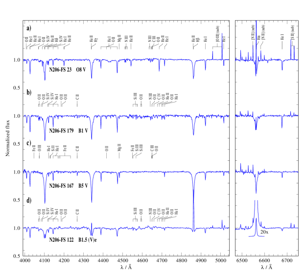
Figure 3: Example spectra of O, early B, late B, and Be stars in the N 206 superbubble. The [O iii], [N ii], and [S ii] lines are from nebular emission (neb).

4 Spectral classification

The spectral classification of OB stars is primarily based on the blue optical wavelength range. We mainly follow the classification schemes proposed in Sota et al. (2011), Sota et al. (2014), and Walborn et al. (2014).

4.1 O stars

We identified 31 O stars in the whole sample (excluding the nine Of stars described in Paper I). The main diagnostic line ratios used for their subtype classification are He i $\lambda 4388$/ He ii $\lambda 4542$, He i $\lambda 4144$/ He ii $\lambda 4200$ and He i $\lambda 4713$/ He ii $\lambda 4686$. An example of an O star spectrum is shown in Fig. 3 (a).

The luminosity-class criteria of O stars are mainly based on the strength of He ii 4686. Two O supergiants are identified in the sample, N206-FS 90 and N206-FS 134. Absent or very weak He ii $\lambda 4686$ absorption together with H$\alpha$ emission reveals their supergiant nature. The Si iv absorption lines are very strong in these spectra. Compared to these objects, N206-FS 62 and N206-FS 192 have stronger He ii $\lambda 4686$ absorption, and therefore are classified as giants. Additionally, these spectra are contaminated with disk emission, suggesting their Oe nature. Furthermore, two main sequence O stars are also identified with Oe features.

We found six stars that exhibit special characteristics typical for the Vz class, namely, N206-FS 64, 107, 145, 154, 184, and 198. According to Walborn (2006), these objects may be near or on the zero-age main sequence (ZAMS). As described in Walborn et al. (2014), the main characteristic of the Vz class is the prominent He ii $\lambda 4686$ absorption feature that is stronger than any other He line in the blue-violet region.

4.2 Early B stars

Stars with spectral subtype B0 to B2 are considered as early B stars in this paper. We identified 102 such stars in the whole sample. The main classification schemes for B stars are taken from Evans et al. (2015) and McEvoy et al. (2015). The classification is based on the ionization equilibrium of helium and silicon. The spectral subtypes are mainly determined from Si iii $\lambda$4553/ Si iv $\lambda$4089 line ratio and the strength of He ii $\lambda 4686$, He ii $\lambda 4542$, and Mg ii $\lambda 4481$. An example of an early B-type spectrum is shown in Fig. 3 (b). Here the Si iii lines are stronger and the He ii lines are weaker than in the O star spectrum in Fig. 3 (a).

For B stars, luminosity classes were mainly determined from the width of the Balmer lines and from the intensity of the silicon absorption lines (Si iv and Si iii). The B supergiants and bright giants show rich absorption-line spectra. For more details on the luminosity and subtype classification, we refer the reader to Table 1 and Table 2 of Evans et al. (2015).

4.3 Late B stars

Stars with spectral subtypes ranging from B2.5 to B9 are considered as late B stars in this paper. We identified a total of 22 such objects. It should be noted that this sample is not complete because of its color and magnitude cut-offs (see Sect. 3). The main diagnostic lines for late B stars are Si ii $\lambda\lambda$4128-4132. We used the line ratios of Si ii $\lambda\lambda$4128-4132 to He i $\lambda 4144$ and of Mg ii $\lambda 4481$ to He i $\lambda 4471$ for classifying their spectral subtypes. An example of a late B-type star (B5 V) is shown in Fig. 3 (c).

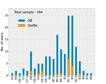
Figure 4: Spectral subtype distribution of all OB stars in our sample. For each spectral subtype, the number of included Oe/Be star is represented in a different color.

4.4 Oe/Be stars

The characteristic features of Oe/Be stars are the strong and broad emission of H$\alpha$ and other Balmer lines (see Fig. 3(d)), which are attributed to a circumstellar decretion disk (Struve 1931) fed by the ejected matter from the central star. We identified 19 such disk-originating emission-line stars in the whole sample, where five of them are classified as Oe stars (including the Oef star in Paper I). Among this Oe/Be sample, three stars are giants or bright giants, while the rest are dwarfs. Most of the Be stars have spectral subtype B1.5–B2.

Thus, the fraction of Oe/Be stars in this region is $\sim$12%. Since the Be stars have a transient nature and the emission line profiles are usually variable, this fraction is just a lower limit. According to McSwain et al. (2008), approximately 25 to 50% of the Be stars may go undetected in a single epoch spectroscopic observation.

The H$\alpha$ and H$\beta$ lines of these Be stars also show different profiles depending on the disk viewing angle (see Rivinius et al. 2013, for more details). Seven stars (N206-FS 9, 119, 121, 122, 181, 192, 233) show H$\alpha$ and H$\beta$ line profiles close to pole-on view. All the other twelve Oe/Be stars show line profiles that indicate higher inclinations because the H$\alpha$ and H$\beta$ emission lines are double-peaked. Four of these stars (N206-FS 62, 113, 186, 192) additionally show characteristics of B[e] stars, defined by Balmer lines in emission plus forbidden emission lines (Lamers et al. 1998).

A histogram of the spectral types of all investigated stars in the superbubble N 206 (including the Of stars from Paper I) is shown in Fig. 4. The number of stars gradually increases with spectral subtypes starting from O2, until B2. One exception is a local maximum at spectral subtype O8. The most populated spectral subtypes are B1.5 and B2. The sudden decrease in the number of stars towards later B subtypes is due to the incompleteness of the sample.

5 Analysis of OB stars

We performed spectral analyses of all OB stars in our sample, determining their physical parameters. This was achieved by reproducing the observed spectra with synthetic spectra, calculated with the Potsdam Wolf-Rayet (PoWR) model atmosphere code.

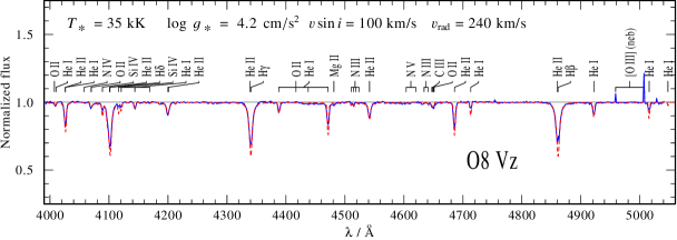
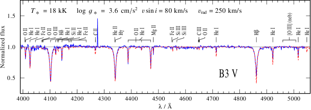
Figure 5: Normalized VLT-FLAMES blue optical spectra (blue solid) for the O star N206-FS 64 (upper panel) and the B star N206-FS 221 (lower panel), respectively. Over-plotted are the synthetic PoWR model spectra (red dashed). The stellar parameters of these best fitting models are given in each panel. The observed spectra are contaminated with nebular emission lines as indicated by “(neb)”.

5.1 The models

The PoWR code for expanding stellar atmospheres is an advanced non-local thermodynamic equilibrium (non-LTE) code that accounts for mass loss, line blanketing, and wind clumping. It can be employed for a wide range of hot stars at arbitrary metallicities (e.g. Hainich et al. 2014, 2015; Oskinova et al. 2011; Shenar et al. 2015), since the hydrostatic and wind regimes of the atmosphere are treated consistently (Sander et al. 2015). The non-LTE radiative transfer is calculated in the co-moving frame. Any model can be specified by its luminosity $L$, stellar temperature $T_{\ast}$, surface gravity $g_{\ast}$, and mass-loss rate $\dot{M}$ as main parameters.

In the subsonic region, the velocity field is defined such that a hydrostatic density stratification is approached (Sander et al. 2015). In the supersonic region, the wind velocity field $\varv(r)$ is pre-specified assuming the so-called $\beta$-law (Castor et al. 1975) with $\beta=0.8$ (Puls et al. 2008). For establishing the non-LTE population numbers, the Doppler broadening $\varv_{\mathrm{Dop}}$ is set to 30 km s^-1 throughout the atmosphere. In the formal integration that yields the synthetic spectra, the Doppler broadening varies with depth and consists of the thermal motion and a “microturbulence” $\xi(r)$. We adopt $\xi(r)=\rm max(\xi_{min},\,0.1\,\varv(r))$ for OB star models with $\rm\xi_{min}=20$ km s^-1 (Shenar et al. 2016). For all the OB stars in our study, we account for wind clumping assuming that clumping starts at the sonic point, increases outwards, and reaches a density contrast of $D=10$ at a radius of $R_{\mathrm{D}}=\,10\,R_{\ast}$. The models account for complex atomic data of H, He, C, N, O, Mg, Si, P, S, and Fe group elements. More details of the PoWR models used for the analysis of our program stars are described in Paper I.

5.2 Spectral fitting

We performed the spectral analysis by iteratively fitting the observed spectra with PoWR models. In order to do that, we constructed OB-star grids with the stellar temperature $T_{\ast}$ and the surface gravity $\log\,g_{\ast}$ as the main parameters. For the metallicity of the LMC, we adopted the values from Trundle et al. (2007). Since the model spectra of OB stars are mostly sensitive to $T_{\ast}$, $\log\,g_{\ast}$, and $L$, these parameters are varied to find the best-fit model systematically. The other parameters, namely the chemical composition and the mass-loss rate, are kept constant within the model grids. The stellar mass $M$ and luminosity $L$ in the grid models are chosen according to the evolutionary tracks calculated by Brott et al. (2011). The LMC OB star grid, which is also available online, spans from $T_{\ast}$ = 13 kK to 54 kK with a spacing of 1 kK, and $\log\,g_{\ast}$ = 2.2 to 4.4 with a spacing of 0.2 dex. For individual stars, we also calculated models with adjusted C, N, O, and Si abundances when necessary. More details about deriving the stellar and wind parameters are described in the following subsections.

5.2.1 Effective temperature

We constrain the stellar temperature mainly from the silicon and helium ionization balance. In the temperature range from 20 to 30 kK, the line ratio Si iii $\lambda$4553/ Si iv $\lambda$4089 decreases with an increase in temperature. In the case of hotter stars ($>$30 kK), the temperature determination is mainly based on the helium line ratios He i $\lambda 4388$/ He ii $\lambda 4542$, He i $\lambda 4144$/ He ii $\lambda 4200$ and He i $\lambda 4713$/ He ii $\lambda 4686$.

For the hottest O stars, where the He i lines are absent or very weak, the temperature diagnostic must rely on nitrogen line ratios (see Paper I). For late B subtypes (13-20 kK), He ii lines are absent. The main diagnostic line, in this case, is the multiplet Si ii $\lambda\lambda$4128-4132, which increases as the stellar temperature goes down from 20 kK to 10 kK. Furthermore, the line ratio Mg ii $\lambda 4481$ to He i $\lambda 4471$ increases with decreasing temperatures and is employed for an accurate determination of the stellar temperature in this range.

As examples, the FLAMES spectra of an O star and a B star are shown in Fig. 5 together with the corresponding PoWR model. The upper panel shows the spectrum of a typical O star with strong He ii lines. The Si iv lines are weak, Si iii lines are absent, and the He i/ He ii ratio is small indicating a high stellar temperature. The observation is reproduced best by a model with $T_{\ast}$ = 35 kK. The lower panel depicts a typical late B star spectrum fitted by a model with $T_{\ast}$= 18 kK. The main indicators are the presence of Si ii absorption lines, strong Mg ii lines, and weak Si iii lines. Here He ii is completely absent and the He i lines are prominent (see Fig. 5).

The fit procedure usually gives a clear preference for one specific grid model. Hence the uncertainty in the temperature determination is limited by the grid resolution of $\pm$1 kK. However, the uncertainty in $\log\,g_{\ast}$ (see below) also propagates to the temperature and leads to a total uncertainty of about $\pm$2 kK.

In the case of Oe/Be stars, the stellar temperature is not of the same precision, because He i, Si iii, and Si ii lines can be partially filled with emission. Furthermore, the Balmer wings are affected by the disk emission, so that a larger uncertainty in $\log\,g_{\ast}$ additionally affects the temperature estimates.

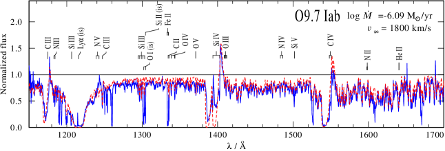
Figure 6: Normalized UV (HST/STIS) spectrum (blue solid line) of an O supergiant (N206-FS 134) is over-plotted with the PoWR model (red dashed line). The wind parameters of this best-fit model are given in the panel. The observed spectrum also contains interstellar absorption lines (is).

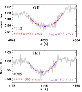
Figure 7: Rotation velocity $\varv$ sin $i$ from the line profile fitting of two fast rotating stars (N206-FS 112 and 209) in the sample using the iacob-broad tool. The gray curves show the observed line profile. The $\varv$ sin $i$ is calculated from line profile fitting based on the Fourier transform method (red dotted line) and goodness-of-fit analysis (violet dashed line). See text for more details.

5.2.2 Surface gravity

The Balmer lines are broadened by the Stark effect; we mainly use their wings to measure the surface gravity $\log\,g_{\ast}$. Since the H$\alpha$ line is often affected by wind emission, H$\gamma$ and H$\delta$ are better suited for this purpose. The typical uncertainty for $\log\,g_{\ast}$ is $\pm$0.2 dex. For example, the Balmer lines of the star shown in the upper panel of Fig. 5 are broad, and the best model fit gives $\log\,g_{\ast}$ = 4.2. The Balmer absorption lines in the observation are less deep than in the model because they are partially filled with nebular emission. Similarly, broad Balmer lines of the B-type star in the lower panel are fitted with a model for $\log\,g_{\ast}$= 3.6, since the stellar temperature is much lower for this object compared to an O star.

For the Oe/Be stars in our sample, the methods described above to measure stellar temperature and $\log\,g_{\ast}$ are not always successful because the equivalent widths of the Balmer lines may be reduced by disk emission. Therefore, the uncertainty in the surface gravity of these stars is relatively high.

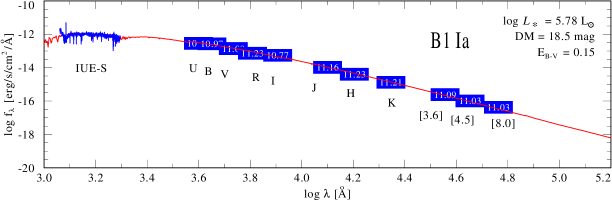
Figure 8: Spectral energy distribution fit of a sample B star (N206-FS 147). The model SED (red) is fitted to the available photometry from optical ($UBVRI$), near-infrared ($JHK_{s}$), and mid-infrared ($IRAC$ 3.6, 4.5, and 8.0 $\rm\mu m$) bands (blue boxes) as well as the flux calibrated UV spectra from the HST. The luminosity $L$ and the color excess $E_{\rm B-V}$ of the best-fitting model are given in the figure.

5.2.3 Mass-loss rate

We calculated two model grids: one with a “high” mass-loss rate of $10^{-7}M_{\odot}\,\mathrm{yr}^{-1}$ and another one with a “low” value of $10^{-8}$ $M_{\odot}\,\mathrm{yr}^{-1}$. The mass-loss rate can be estimated from the P-Cygni profiles of the UV resonance lines. For eight of our sample stars, UV spectra are available. The main diagnostic lines are the resonance doublets C iv $\lambda\lambda$1548–1551 and Si iv $\lambda\lambda$1393–1403 in the HST / IUE range. Useful wind lines in the FUSE range are P v $\lambda\lambda$1118–1128, C iv $\lambda$1169, and C iii $\lambda$1176.

As an example, the UV spectrum of the O supergiant N206-FS 134 is shown in Fig. 6. The normalized high-resolution HST/STIS data are fitted with a PoWR model. This spectrum was consistently normalized with the reddened model continuum. The mass-loss rate is estimated to be $\log\dot{M}$ = -6.1 [$M_{\odot}\,\mathrm{yr}^{-1}$], on the basis of the shown UV fit and in accordance with H$\alpha$.

Without UV spectra, the mass-loss rate estimates can only rely on wind emission in H$\alpha$ and He ii $\lambda 4686$. In case we have UV observations or, at least, the H$\alpha$ line is in emission, we calculate additional models with adjusted mass-loss rates for the individual stars and precisely determine $\dot{M}$. The error in $\log\dot{M}$ is approximately $\pm$0.1 dex if obtained with the help of UV spectra, and $\pm$0.2 dex if only based on H$\alpha$ and He ii$\lambda 4686$.

Most of the stars in our sample have neither H$\alpha$ in emission nor available UV spectra. In these cases, we adopt the “high” mass-loss rate of $10^{-7}M_{\odot}\,\mathrm{yr}^{-1}$ for the O stars and the“low” $\dot{M}=10^{-8}M_{\odot}\,\mathrm{yr}^{-1}$ for B stars and consider these values as upper limits.

5.2.4 Terminal velocity

For stars with available UV spectra, we measured the terminal velocities ($\varv_{\infty}$) from the blue edge of the absorption trough of the P-Cygni profiles and recalculated the models accordingly. The main diagnostic P-Cygni profiles are from the doublets C iv $\lambda\lambda$1548–1551, P v $\lambda\lambda$1118–1128, and S v $\lambda\lambda$1122–1134. The typical uncertainties in $\varv_{\infty}$ from these measurements are $\pm$ 100 km s^-1. Figure 6 shows an example UV spectrum, where $\varv_{\infty}$ is measured from the best fit of the blue edge of C iv $\lambda\lambda$1548–1551 as $1800\pm 50$ km s^-1. Since this line is saturated, it is not sensitive to clumping.

For those stars for which we have only optical spectra, the terminal velocities are estimated theoretically from the escape velocity $\varv_{\mathrm{esc}}$. The ratio between terminal and escape velocity has been studied for Galactic massive stars both theoretically and observationally and found to be $\varv_{\infty}$/$\varv_{\mathrm{esc}}\simeq$ 2.6 for stars with $T_{\ast}\geq$ 21 kK, while for stars with $T_{\ast}<$ 21 kK the ratio is $\approx$1.3 (Lamers et al. 1995; Kudritzki & Puls 2000). The terminal velocity is expected to depend slightly on metallicity, $\varv_{\infty}\,\propto(Z/Z_{\odot})^{q}$, where $q=0.13$ (Leitherer et al. 1992), and we adopted this scaling to account for the LMC metallicity.

5.2.5 Radial velocity

We measured the radial velocity of all sample stars based on the absorption lines in the VLT-FLAMES spectra. These measurements are performed manually by fitting a number of line centers of the synthetic spectra to the observation. Generally, hydrogen lines are poor indicators for radial velocity measurements, because they are broad, sensitive to wind effects, and possibly affected by nebular emission (Sana et al. 2013b). Metal lines, on the other hand, are very weak in O-star spectra. So, we can use Si and Mg lines to measure radial velocity only in B- star spectra . Mainly, we use the He i lines at 4026, 4387, 4471, and 4922 Å and the He ii lines at 4200 and 4541 Å for measuring the radial velocities. Examples can be seen in Fig. 5, where the radial velocity for the O star (upper panel) is estimated to be 240 km s^-1 and for the B star to be 250 km s^-1 (lower panel).

The typical uncertainty of $\varv_{\rm rad}$ is about $\pm$10 km s^-1. However, in a few cases, where stars have large rotational velocities or the spectra are noisy, the precise determination of the line centers is more difficult and the uncertainty can increase up to $\pm$20 km s^-1.

5.2.6 Projected rotational velocity

We constrain the projected rotation velocity $\varv\,\sin i$ of all OB stars from the line profile shapes, using the iacob-broad tool written in IDL (Simón-Díaz & Herrero 2014). The $\varv\,\sin i$ measurements are mainly based on absorption lines in the blue optical wavelengths. We used both implemented methods, the combined Fourier transform (FT) and the goodness-of-fit (GOF) analysis, as described in Paper I.

The primary lines selected for applying these methods are He i, Si iv and Si iii. The lines used for measuring $\varv\,\sin i$ of O-stars are He i lines at 4026, 4387, 4471, and 4922 Å, and Si iv lines at 4089 and 4116 Å. For B stars, we used He i lines at 4144, 4387, 4471 and 4922 Å, the C ii line at 4267 Å, the Mg ii line at 4481 Å, Si iii lines at 4552 to 4575 Å, the O ii line at 4649 Å, and the N iii line at 4641 Å.

Figure 7 shows rotationally broadened lines from two stars of our sample with the fastest rotation, N206-FS 112 and N206-FS 209 respectively. These stars are rotating close to their critical velocity (approximately $0.7\,\varv_{\rm critical}$). The typical uncertainty in $\varv\,\sin i$ is $\sim$ 10%. Finally, we adopt these measured velocities and convolve our model spectra to account for rotational and macroturbulent broadening. This leads to line profile fits consistent with the observations (e.g., Fig 5) in all cases.

5.2.7 Luminosity and reddening

The luminosity $L$ and the color excess $E_{\rm B-V}$ of the individual OB stars were determined by fitting the model SED to the photometry. The model flux is diluted with the LMC distance modulus of 18.5 mag (Pietrzyński et al. 2013). The uncertainty in the luminosity depends on the uncertainty in the color excess (which is typically small for LMC stars), the temperature, and the observed photometry. The total uncertainty is about 0.2 in $\log\,L$. If flux-calibrated UV spectra (HST, IUE, or FUSE) are available, this gives additional information on the SED, and the uncertainty in the luminosity is only $\approx$0.1 dex in these cases.

An example SED fit of a B supergiant is given in Fig. 8. The figure shows the theoretical SED fitted to multi-band photometry and flux calibrated UV spectra. We appropriately adjusted the reddening and the luminosity of the model’s SED to the observed data. Reddening includes the contribution from the Galactic foreground ($E_{\rm B-V}$ = 0.04 mag) adopting the reddening law from Seaton (1979), and from the LMC using the reddening law described in Howarth (1983) with $R_{V}=3.2$. The total $E_{\rm B-V}$ is a fitting parameter.

Table 2 summarizes the main diagnostic lines used for the different aspects of the fitting process. This iterative procedure yields the stellar and wind parameters of the O, early B and late B stars in our sample. In the course of this procedure, individual models with refined stellar parameters and abundances are calculated for each of these stars. The fitting process is iterated until no further improvement of the fit is possible.

Table 2: Main diagnostics used in our spectral fitting process.

Parameter	O stars	Early B stars	Late B stars
$T_{\ast}$	He i/He ii line ratios	Si iii/Si iv line ratios	Si ii/Si iii, Mg ii/He i line ratios
$\log\,g_{\ast}$	H$\gamma$ and H$\delta$ line wings	H$\gamma$ and H$\delta$ line wings	H$\gamma$ and H$\delta$ line wings
$\dot{M}$	H$\alpha$, He ii 4686, Si iv 1393–1403	H$\alpha$, He ii 4686, Si iv 1393–1403	H$\alpha$, He ii 4686, Si iv 1393–1403
	P v 1118–1128, C iv 1169, C iii 1176	C iv 1548–1551
	C iv 1548–1551
$\varv_{\infty}$	H$\alpha$, N v 1238–1242, C iv 1548–1551	H$\alpha$, C iv 1548–1551	H$\alpha$, Si iv 1393–1403
	Si iv 1393–1403, P v 1118–1128	Si iv 1393–1403
$\varv\,\sin i$	He i lines, N iii 4510–4525	He i lines, N iii 4641	He i lines, C ii 4267
	Si iv 4089–4116	Si iii 4552–4575, O ii 4649	Mg ii 4481
$\varv_{\rm rad}$	He i and He ii lines	He i lines, Si iii 4552–4575	He i lines, C ii 4267, Mg ii 4481

Table 3: Stellar parameters of OB stars in N 206

N206-FS	Spectral type	$T_{\ast}$	$\log\,L$	$\log\,g_{\ast}$	$\log\,\dot{M}$	$E_{\rm B-V}$	$M_{\mathrm{V}}$	$R_{\ast}$	$\varv_{\infty}$	$\varv$ sin $i$	$\varv_{\rm rad}$	$M_{\ast}$	$\log\,Q_{0}$	$L_{\mathrm{mec}}$
#		[kK]	[$L_{\odot}$]	[cm s-2]	[$M_{\odot}\,\mathrm{yr}^{-1}$]	[mag]	[mag]	[$R_{\odot}$]	[km s-1]	[km s-1]	[km s-1]	[$M_{\odot}$]	[s-1]	[$L_{\odot}$]
1	B1.5 V	20.0	4.23	3.6	-7.78	0.18	-3.96	10.9	800	100	280	17	45.7	0.9
3	B2.5 IV	18.0	3.93	3.6	-8.00	0.12	-3.29	9.5	800	130	250	13	45.4	0.5
5	B1 V	25.0	4.06	4.2	-7.78	0.12	-2.67	5.7	2500	100	270	19	46.3	8.7
6	B2.5 IV	20.0	4.13	3.6	-7.85	0.12	-3.50	9.7	800	180	280	14	45.6	0.7
7	B0.5 V	29.0	4.44	4.2	-6.78	0.08	-3.64	6.6	2500	229	240	25	47.2	86.6
9	B1.5 (III)e	20.0	4.48	3.2	-7.00	0.25	-4.20	14.5	600	130	290	12	46.5	3.0
10	B0.5 V	27.0	4.22	4.2	-6.80	0.05	-3.12	5.9	2400	90	250	20	46.6	74.5
11	B2 IV	21.0	4.20	3.8	-7.70	0.10	-3.61	9.5	2000	120	280	21	45.8	6.6
12	B2.5 IV	20.0	4.38	3.6	-7.66	0.24	-3.98	12.9	900	80	260	24	45.9	1.5
14	B2 (IV)e	20.0	4.43	3.6	-7.62	0.18	-4.03	13.7	1000	130	260	27	46.0	2.0
15	B2.5 IV	19.0	3.93	3.8	-8.00	0.13	-3.24	8.5	1000	90	250	17	45.3	0.8
17	B2 IV	20.0	4.33	3.6	-7.70	0.23	-3.71	12.2	900	160	260	22	45.8	1.3
19	B2.5 IV	18.0	4.03	3.4	-7.93	0.12	-3.42	10.7	700	160	280	10	45.4	0.5
22	B2.5 V	20.0	4.13	3.6	-7.85	0.08	-3.29	9.7	800	80	240	14	45.6	0.7
23	O8 V	35.0	4.86	4.2	-6.65	0.24	-3.79	7.3	2500	60	230	31	48.3	115.5
27	O9.5 IV	32.0	4.76	4.0	-6.93	0.20	-4.11	7.8	1900	21	280	22	47.9	35.4
28	B7 IV	14.0	3.86	3.4	-8.11	0.22	-3.47	14.5	800	90	240	19	44.9	0.4
29	B5 IV	17.0	3.60	3.6	-8.15	0.12	-2.78	7.3	700	120	280	8	45.0	0.3
30	B0.5 V	27.0	4.16	4.2	-6.85	0.08	-2.86	5.5	2300	75	250	18	46.6	61.7

6 Analysis of WR binaries

The two WR binaries present in this region are analyzed using PoWR models. The detailed analysis of the binary system N206-FS 45 (BAT99 49) with spectral type WN4:b+O will be given in Shenar et al. (in prep.), and we are adopting the derived parameters in this paper. The second binary, N206-FS 128 (BAT99 53), is classified as WC4+O (Bartzakos et al. 2001; Kavanagh et al. 2012). We perform the analysis of this WC star using our LMC-WC grid models. Most of the descriptions of PoWR models given in Sect. 5.1 are also applicable in the case of WR stars, with few special aspects as given below.

6.1 The model

In the case of WR models, the parameter $\log\,g_{\ast}$ is not as important as for OB star models, since the spectral lines originate primarily in the wind. The outer boundary is taken to be $R_{\rm max}$=1000 $R_{*}$ for WR models. Accounting for the very strong microturbulence in WR winds, the Doppler velocity is set to 100 km/s (e.g. Hamann et al. 2006). For the velocity law exponent (see Equation 2 in Paper I), we adopt $\beta$ = 1 as usual for WR winds.

For the chemical composition of the WC star, we assume mass fractions of 55% helium, 40% carbon, 5% oxygen, 0.1% neon, and 0.07% iron-group elements. For the published WC grid, the terminal wind velocity was set to 2000 km/s. For the WC star in N206-FS 128, we calculated models with higher terminal velocities to fit the spectrum.

Table 4: Stellar parameters of WR binaries in N 206

N206-FS	Spectral type	$T_{\ast}$	$\log\,L$	$\log\,g_{\ast}$	$\log\,\dot{M}$	$E_{\rm B-V}$	$D$	$R_{\ast}$	$\varv_{\infty}$	$\varv$ sin $i$	$\varv_{\rm rad}$	$M_{\ast}$	$\log\,Q_{0}$	$L_{\mathrm{mec}}$
#		[kK]	[$L_{\odot}$]	[cm s-2]	[$M_{\odot}\,\mathrm{yr}^{-1}$]	[mag]		[$R_{\odot}$]	[km s-1]	[km s-1]	[km s-1]	[$M_{\odot}$]	[s-1]	[$L_{\odot}$]
45	WN4:b	100	5.4	5	-5.4	0.1	10	1.6	1700	-	250	18	49.3	955
	O8 III	33	5.2	3.6	-7.0	0.1	10	12.2	2100	280	250	27	48.8	37
128	WC4	158	5.35	6.0	-4.67	0.1	40	0.6	3400	-	220	13	49.1	20400
	O9 V	33	5.22	3.8	-7.0	0.1	10	11.3	2400	200	220	29	48.5	27

Figure 9: Histograms of stellar temperature, surface gravity, color excess, projected rotational velocity, radial velocity, stellar mass, mass-loss rate, and mechanical luminosity of OB stars in N 206 superbubble. The number of stars in the y-axis are shown in logarithmic scale. We used the square root (of data size) estimator method to calculate the optimal bin width and consequently the number of bins.

6.2 Spectral fitting

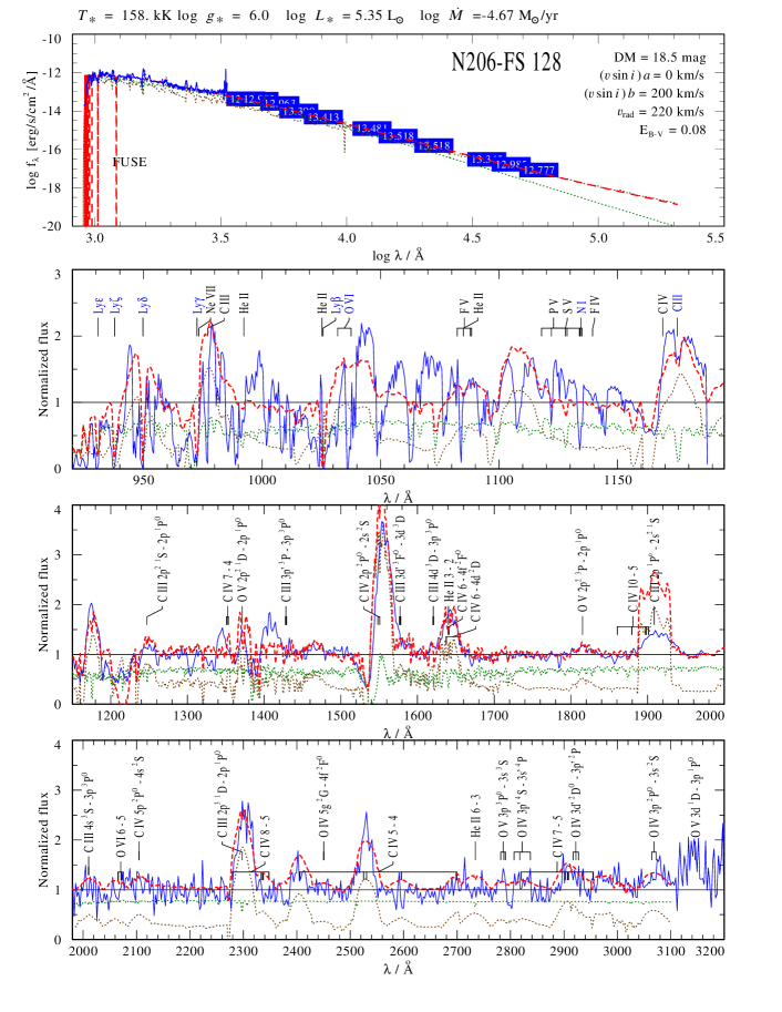
Figure 29: Spectral fit for N206-FS 128. The upper panel shows the spectral energy distribution with photometry from UV, optical, and infrared bands as well as the flux calibrated UV spectra. Lower panels show the normalized UV spectra from FUSE, IUE-short, and IUE-long (blue solid lines), fitted by composite model (red dashed lines). The WC and O star models are represented with brown and green dotted lines respectively.

The observed spectrum is a sum of a WC spectrum and an O star spectrum (see Fig. 29 and 30). In order to reproduce this, we add the fluxes of a WC and an O star model. The light ratio is mainly constrained by the strength of the He i absorption features which are clearly associated with the O star component (secondary), while the broad emission features are from the WC star (primary). For fitting the light ratio, we separately adjust the luminosities of both stars, under the constraint that the sum of the fluxes, after reddening, fits the observed SED (see Fig. 29).

The main diagnostic of the temperature of the WC star is the C iii to C iv line ratio. The C iv $\lambda$5808 emission is stronger than the C iii $\lambda$4648 emission. The strong O v line emission also indicates a very high stellar temperature ($>$100 kK). The best-fit model has a temperature of 158 kK. The terminal velocity is determined to be $\sim 3400$ km $\rm s^{-1}$, based on the width of the prominent C iii and C iv features in the UV and optical spectra. The clumping contrast $D$ must be chosen as high as 40. With the standard value of $D=10$ (Sander et al. 2012), the model predicts much stronger electron scattering wings of the blend complex at $\lambda\approx$4686 Å and the C iv line at 7721 Å. Most of the emission lines in the spectra are reproduced by a model with a mass-loss rate of $2\times 10^{-5}\,M_{\odot}\,\mathrm{yr}^{-1}$. The effective temperature of the O star, $T_{\ast}=33$ kK, is derived from the ratio between the He i and He ii absorption lines.

For the WC component, our final model has a luminosity of $\log\,L=5.35\,L_{\odot}$, which is relatively low compared to that of single WC stars in the LMC (Crowther et al. 2002). However, stars of the same spectral type in the Milky Way show such low luminosities (Sander et al. 2012). The O star component has a luminosity of $\log\,L=5.22\,L_{\odot}$, which corresponds to luminosity class V.

7 Results and discussions

7.1 Stellar parameters

The fundamental parameters for the individual stars are given in Table 3. The rate of hydrogen ionizing photons ($\log\,Q_{0}$) and the rate at which the kinetic energy is carried away by the stellar winds (mechanical luminosity $L_{\mathrm{mec}}\,=\,0.5\,\dot{M}\,\varv_{\infty}^{2}$) are also tabulated. The derived parameters of the WR binaries are compiled in Table 4.

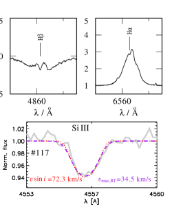
Figure 10: Upper panel shows the H$\beta$ and H$\alpha$ line profiles of one of the slow rotating Be stars, N206-FS 117. The lower panel shows $\varv$ sin $i$ from the profile fitting of the Si iii absorption line using the iacob-broad tool. The gray curves show the observed line profile. The $\varv$ sin $i$ is calculated from line profile fitting based on the Fourier transform method (red dotted line) and goodness-of-fit analysis (violet dashed line).

For the whole sample, we plot histograms for the distributions of stellar temperature, surface gravity, color excess, projected rotational velocity, radial velocity, stellar mass, mass-loss rate, and mechanical luminosity (Fig. 9). The stellar temperature of the OB stars (including the Of stars) ranges from 14 to 50 kK. In the surface gravity histogram (Fig. 9), most of the stars are found at surface gravities $\log\,g_{\ast}$ between 4.0 and 4.2. Only 15% of the stars have log g $\leq$ 3.4 cm s^-2, indicating giants or supergiants. The color excess histogram reveals that most of the stars in the N 206 superbubble have a very low color excess of $E_{\rm B-V}\approx 0.1$. Stars that belong to the young cluster NGC 2018 are found to have comparatively higher extinction, with five cluster members showing $E_{\rm B-V}>0.25$. These young stars in the cluster are still surrounded by the reminder of their parental cloud. This is consistent with the far infrared Herschel images and CO intensity maps that reveal a distribution of cold dense gas around this cluster (see Fig. 28).

The histogram of the stellar masses (Fig. 9) refers to spectroscopic masses, calculated from $\log\,g_{\ast}$ and $R_{\ast}$ ($g_{\ast}=G\,M_{\ast}\,R_{\ast}^{-2}$). These masses vary in the range of $7-150\,M_{\odot}$. The number of objects decreases with increasing mass. We note that the lowest mass bin is not complete.

From the mass-loss rate histogram, we can see that the OB stars in the sample have log $\dot{M}$ [$M_{\odot}\rm{yr^{-1}}$] in the range of $-8.5$ to $-4.8$. Stars with the highest mass-loss rates are either super-giants or bright giants. The statistics of the mechanical luminosity, $L_{\rm mec}=0.5\dot{M}\varv_{\infty}^{2}$, are also plotted as a histogram in Fig. 9. This distribution suggests that most of the OB stars in our sample release $L_{\rm mec}<20\,L_{\odot}$ to the surrounding ISM. This is $10-100$ times lower than the mechanical luminosities of any of the Of stars analyzed in Paper I. The mechanical luminosities of the WR stars are even larger (see below).

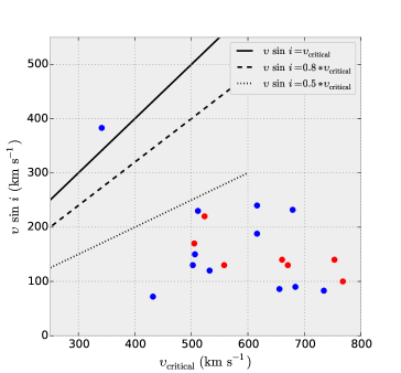
Figure 11: Projected rotational velocity ($\varv\sin i$) versus critical velocity ($\varv_{\rm critical}$) of Oe/Be stars. The red dots represent stars with a pole-on view as deduced from the H$\beta$ and H$\alpha$ line profiles, while the remaining stars are represented by blue dots. The solid, dashed, and dotted lines represent 100%, 80%, and 50% of $\varv_{\rm critical}$, respectively.

7.1.1 Stellar rotation

The distribution of projected rotational velocities ($\varv\sin i$) covers 30 to 400 km s^-1 (Fig. 9, bottom). Most of the stars have a $\varv\sin i$ of around $\sim$100 km s^-1. The presence of a low-velocity peak and a high-velocity tail is consistent with studies of other massive star forming regions (Ramírez-Agudelo et al. 2013; Penny 1996).

Fifteen OB stars of the sample are rotating faster than 200 km s^-1, and five of them (3%) exhibit very fast rotation with $\varv\sin i$ in the range 340-400 km s^-1. Interestingly, only the Oe star, N206-FS 62, is rotating very fast. All other 18 Oe/Be stars in our sample show only a moderately enhanced rotation with an average $\varv\sin i$ of about 160 km $\rm s^{-1}$, while the average for the other B stars is $\approx 120$ km $\rm s^{-1}$. As an example, the line profiles and projected rotational velocity measurements of one of the sample Be stars with slow rotation are shown in Fig. 10.

For the Oe/Be stars in our sample, we compared $\varv\sin i$ with the critical rotational velocity $\varv_{\rm critical}=(2GM_{\ast}/(3R_{\ast}))^{0.5}$ (see Fig. 11). Interestingly, most of the Oe/Be stars rotate significantly below their critical velocity with $\varv\sin i$ $\sim(0.1\ldots 0.5)\,\varv_{\rm critical}$. Here $\varv_{\rm critical}$ is calculated from the spectroscopic masses. For a comparison, we also calculated the critical velocities using evolutionary masses, which are generally lower (see Sect. 7.3). Even in this case, 75% of the Oe/Be stars are rotating with $\varv\sin i\,<0.5\,\varv_{\rm critical}$.

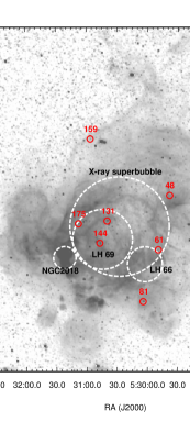
Figure 12: Eight candidate runaway OB stars in the sample. The underlying H$\alpha$ image is from the Magellanic Cloud Emission-Line Survey (MCELS, Smith et al. 2005).

Table 5: Candidate runaway OB stars in the N 206 superbubble

N206-FS	$\varv_{\rm rad}$	$\varv_{\rm rad}$ - $\bar{\varv}_{\rm rad}$	spectral type
#	(km s-1)	(km s-1)
9	300	52	B1.5 (IV)e
48	180	$-68$	B0.7 V
61	180	$-68$	B0.7 V
81	160	$-88$	B1 II
131	185	$-63$	O6.5 II (f)
144	320	72	B0 II Nwk
159	320	72	B2 V
175	330	82	B0 III

The Oe and Be stars in our sample in general rotate sub-critically. Our result is in line with the statistical study by Cranmer (2005) who concluded that this strongly constrains the physical models of angular momentum deposition in Be star disks. However, many observations of Be stars in the Galaxy and Magellanic Clouds suggest that most of them are rotating at almost their critical velocity (Rivinius et al. 2013; Martayan et al. 2006, 2010).

One possible reason for finding a low $\varv\sin i$ could be an accidental pole-on view ($\sin i\approx 0$). From inspecting the Balmer emission line profiles, we distinguish between double-peak disk emissions and single peaks. For the latter, one may suggest a low inclination angle. Typically, the disk emission of H$\alpha$ shows up by double peaks that are separated by up to 4 Å in the case of large inclination. Given the limited spectral resolution of our data, we cannot resolve double peaks with separations below 0.8 Å. Therefore, our category of pole-on stars (red dots in Fig. 11) comprises stars with $\sin i\leq 0.2$ corresponding to $i\leq 10\degr$.

However, the statistically probability of observing an inclination below the angle $i$ scales with $1-\cos i$. This implies that the chance of catching a star with an inclination $i\leq 10\degr$ is only about 2%. The likely reason that we find seven out of 19 Oe/Be stars with apparently low inclination is the contamination by nebular emission, so that the double peaks of the Balmer profiles cannot be recognized. Nevertheless, it is puzzling that nearly all Oe/Be stars of the sample with higher inclination also show $\varv\sin i<0.5\,\varv_{\rm critical}$. The only exception is N206-FS 62, which rotates close to its critical velocity.

7.1.2 Radial velocity and candidate runaway stars

The radial velocity of OB stars in our N 206 sample ranges from 160 to 330 km s^-1 (see Fig. 9), with a peak of the distribution at about $\sim$240-270 km s^-1. Runaway stars are usually defined by peculiar velocities in excess of 40 km/s (Blaauw 1961) compared to the systemic velocity. Their velocity is either a result of dynamical ejection from a young cluster or of ejection from a binary system due to a supernova.

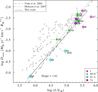
Figure 13: Modified wind momentum ($D_{\mathrm{mom}}$) in units of $M_{\odot}$/yr km s${}^{-1}\,R_{\odot}^{0.5}$ as a function of stellar luminosity for analyzed LMC OB stars. The filled and hatched symbols are wind momenta determined from H$\alpha$ or nitrogen emission lines and from UV P-Cygni profiles with individual error bars, while open triangles (up-side down) indicate upper limits. A power-law (solid line) fit to the observations yields a slope of 1.61. The theoretical WLR from Vink et al. (2000) (dashed line) and an empirical WLR from Mokiem et al. (2007) for LMC stars are also plotted. Luminosity classes are distinguished by different symbols as given in the legend.

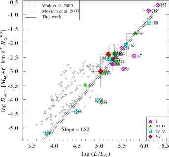
Figure 14: Same as Fig. 13, but including the Of stars from Paper I.

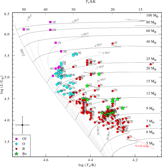
Figure 15: Hertzsprung-Russell diagram for OB stars in the N 206 superbubble in the LMC. The nine Of stars from Paper I are also included. The evolutionary tracks (thin solid lines) are labeled with their initial mass. Isochrones are represented by gray dotted lines. Tracks and isochrones are based on evolutionary models accounting for rotation with $\varv_{\mathrm{rot,init}}\,\sim$ 100 km s^-1 (Brott et al. 2011; Köhler et al. 2015). Different spectral types are distinguished by different colors and shapes of the symbols (see legend). The typical uncertainties of the stellar temperatures and luminosities are indicated by the error bars in the lower left of the HRD. The red dotted line represents the visual-magnitude cut-off of the observed sample.

To identify runaway candidates in our sample, we compared the radial velocity estimates for each star with the mean radial velocity of all program stars and the corresponding standard deviation. By accounting for a threshold of $|\delta\varv_{\rm rad}|>3\sigma$, we identify runaway candidates. Then we recalculate the mean velocity and standard deviation excluding these objects, continuing this process until no more stars with $|\delta\varv_{\rm rad}|>3\sigma$ remain. We find eight runaway candidates among the total sample. This includes the Of binary N206-FS 131 described in Paper I. All other runaways are early B-type stars. Their positions are marked in Fig. 12; their radial velocities as well as the deviation from the mean velocity are given in Table 5.

The mean radial velocity of the OB stars (excluding the runaway candidates) in this region is found to be $\approx$248$\pm$16 km s^-1. This dispersion of $\pm 16\,$km s^-1 includes the $\pm 10\,$km s^-1 uncertainty of the $\varv_{\rm rad}$ measurement, meaning that the actual velocity dispersion is smaller. The radial velocities do not show any obvious correlation with spatial structures in the complex.

7.2 The wind momentum-luminosity relationship

We quantitatively investigate the wind properties of our sample OB stars by plotting the modified wind momentum-luminosity relation (WLR) and compared our results to previous studies and theoretical predictions. Figure 13 depicts the modified stellar wind momentum, which is defined as $D_{\mathrm{mom}}\equiv\dot{M}\varv_{\infty}R_{\ast}$ (Kudritzki & Puls 2000), as a function of the stellar luminosity. The wind momentum of eight stars, which have available UV spectra, and nine OB stars with H$\alpha$ partially or completely in emission, are empirically determined and plotted in the figure. For all other stars, only an upper limit for the wind momentum can be estimated, as marked by upside-down triangles. A linear regression to the logarithmic values of the modified wind momenta obtained in this work, accounting for the individual error bars, gives a slope of $1.61\pm 0.22$, which is less steep than the theoretically predicted slope of 1.83 for LMC OB stars (Vink et al. 2000) given in Fig. 13 (dashed line). The empirical WLR obtained by Mokiem et al. (2007) for LMC OB stars with a slope of 1.81 is also marked in the figure (dotted line) for comparison. Figure 14 shows the WLR of the whole OB star sample including the Of stars from Paper I. This yields a linear regression of

$$\log\,D_{\mathrm{mom}}\,=\,(1.82\pm 0.18)\,\log\,(L_{\ast}/L_{\odot})\,+\,(-12.25\pm 0.95)$$ (1)

which is close to the theoretical and empirical relations shown.

However, this agreement might be just fortuitous. First of all, the empirical wind momenta show a large scatter. Moreover, they are based on different diagnostics, which have their specific issues. The Balmer line emission is fed by the recombination cascade and therefore subject to the microclumping effect. The empirical mass-loss rate derived from a given observed emission line scales roughly with the square root of the adopted clumping contrast (e.g. Hamann & Koesterke 1998). For our analyses, we adopted a clumping contrast of $D=10$, while the WLR from Mokiem et al. (2007) shown in Figs. 13 and 14 have been obtained with smooth-wind models.

On the other hand, part of our empirical mass-loss rates have been derived from fitting the P-Cygni profiles of UV lines (hatched symbol filling in Figs. 13 and 14). These resonance lines are not affected by microclumping, but here the usual neglect of macroclumping (“porosity”) can lead to an underestimation of mass-loss rates (Oskinova et al. 2007).

Another uncertainty refers to the actual metallicity of the individual stars. The theoretical prediction from Vink et al. (2000) has been calculated for a canonical LMC metallicity of 0.5 solar. Our young stars, and especially the two most luminous Of stars in our sample, might have formed already with higher metallicity. Our spectral data allow only very limited abundance measurements, and the total metallicity cannot be precisely determined. On the other hand, Vink mass-loss rates have been often found to over-predict $\dot{M}$ by about a factor of two for early OB-type stars (e.g. Šurlan et al. 2013) and by more than an order of magnitude for late OB-type stars (Martins et al. 2009; Shenar et al. 2017).

7.3 OB stars in the Hertzsprung-Russell diagram

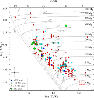
Figure 16: Same as Fig. 15 with symbol shapes and colors referring to the projected rotational velocity (see legend).

The evolutionary status of all hot OB stars in the N 206 complex are investigated using the Hertzsprung-Russell diagram (HRD). Figure 15 shows our sample of OB stars with the effective temperatures and luminosities as given in Table 3. The nine ‘Of stars’ from Paper I are also included.

The evolutionary tracks and isochrones are adapted from Brott et al. (2011) and Köhler et al. (2015), which were calculated for an initial rotational velocity of $\sim$ 100 km s^-1. This seems roughly adequate since the $\varv\sin i$ histogram in Fig. 9 revealed an average of $\sim$ 126 km s^-1. The evolutionary tracks are shown for stars with initial masses of 5 $-$ 100 $M_{\odot}$, while the isochrones are shown for ages of 0, 1, 2, 3, 4  5, 7, 10, 20, and 30 Myr, respectively.

Figure 15 shows that most of the O stars have ages between 1 and 7 Myr, with initial evolutionary masses ranging from 15 to 40 $M_{\odot}$. In the case of B stars, ages extend from 5 to 30 Myr. Interestingly, most of the Be stars are close to the terminal age main sequence as indicated by the loops in the evolutionary tracks.

The most massive stars in our sample (N206-FS180, 187, and 214) are the youngest ones. This supports a scenario described in Bouret et al. (2013), where the most massive stars of the cluster form last, and after their formation, they quench subsequent star formation. However, our finding could also be due to the V-magnitude ($V<16$ mag) cut-off of the sample, since we might miss very young B-type stars.

Figure 16 shows also the HRD of the OB stars, but now color-coded with their respective projected rotational velocity. Five fast rotators with $\varv\sin i>$300 km s^-1 (N206-FS 62, 112, 155, 190, and 209) are found to have initial evolutionary masses less than 20 $M_{\odot}$ (see dark-blue circles in the diagram). The most massive and youngest stars ($<$5 Myr) are found to be slower rotators than the rest of the sample. Interestingly, one slow rotator (N206-FS 52) with $\varv\sin i\approx$35 km s^-1 and the fastest rotator (N206-FS 112) with $\varv\sin i\approx$390 km s^-1 fall on nearly the same position in the HRD. However, both of these stars have similar spectral type and mass.

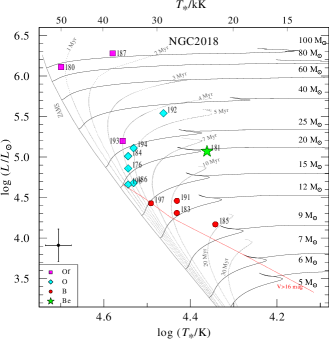
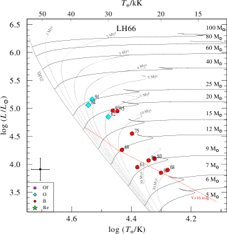
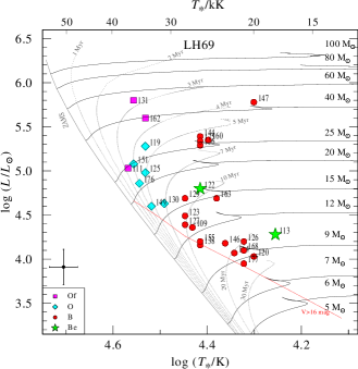
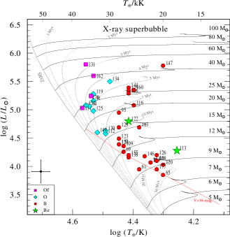
Figure 17: Hertzsprung-Russell diagram for stars in subregions of N 206 (circular regions shown for NGC 2018, LH 66, LH 69, and X-ray superbubble in Fig. 1). The evolutionary tracks, isochrones, and symbols have the same meaning as in Fig. 15.

7.3.1 HR diagram of substructures

As discussed above, the empirical HRD indicates a spread of stellar ages rather than a coeval population of OB stars. This raises the question of multiple or progressing star formation throughout this large region. Therefore, we split our sample into different spatial regions as given in Fig. 1, and plot their respective HRDs (Fig. 17).

The upper-left panel refers to the cluster NGC 2018, which contains mostly O stars and especially the three most massive stars of the whole sample. Most of the stars in this cluster fall in the age range of $2-4$ Myr. The cluster shows a large age dispersion from $\leq$1 Myr (N206-FS180) to $\sim$20 Myr (N206-FS185).

Most stars in the OB association LH 66 (Fig. 17, upper-right panel) have ages in the range $7-10$ Myr, with no star being younger than 5 Myr. The OB association LH 69 (lower-left panel) contains multiple populations with ages of 4, 5, 10, and 20 Myr. The youngest star in this association is $\leq$3 Myr old. Most of the stars in LH 69 are part of the somewhat larger X-ray superbubble region, which shows an age dispersion in the range $3-30$ Myr.

Summarizing this investigation revealed that each of the subregions of the N 206 complex had multiple episodes of star formation over the last 30 Myr. However, only the cluster NGC 2018 formed stars as recently as 1 Myr ago.

7.3.2 The evolutionary status of the WC+O binary N206-FS 128

We compare the HRD positions of the binary components of N206-FS 128 with evolutionary tracks from Eldridge et al. (2008), which account for binary interaction (see Fig. 18). These binary tracks are defined by three parameters : the initial mass of the primary $M_{i,1}$, the initial orbital period $P_{i}$, and the mass ratio $q_{i}=M_{i,2}/M_{i,1}$. Using the $\chi^{2}$ minimization algorithm described in Shenar et al. (2016), we found the best fitting parameters for the binary track to be $M_{i,1}=35M_{\odot}$, $P_{i}=10$ days, and $q_{i}=0.7$. After 6 Myr of evolution, this binary track reproduces not only the observed HRD positions but also the current surface hydrogen and carbon abundances of both components very well. The current period of the binary system predicted by the model is $\approx 5$ days, and thus slightly higher than the observed value of 3.23 days measured by Mowlavi et al. (2017).

According to the best-fitting binary track, the WC component N206-FS 128a started its evolution with an initial mass of $35M_{\odot}$ and stayed on the main sequence (pre WR phase) for 5.4 Myr. Before it entered into the WR phase, it had undergone a Roche lobe overflow (RLOF) phase (dashed magenta lines in Fig. 18) over $\sim$20,000 years. During this phase, the primary looses more than half of its mass, and the secondary accretes a few solar masses. After this, N206-FS 128a entered the WNL stage with a low hydrogen mass fraction $0<X_{\rm H}<0.2$ at the surface. The WNE phase is reached when the surface hydrogen has vanished. When the helium-burning products appear at the surface, the star proceeds to the WC/WO phase.

During the last 0.6 Myr, the primary experienced very high mass loss, which decreased its mass to about 10 $M_{\odot}$, while the mass of the secondary remained roughly constant. This is the current state of the system, at an estimated age of roughly 6 Myr.

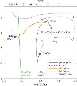
Figure 18: HRD positions of N206-FS 128a (WC4, blue asterisk) and N206-FS 128b (O9, red square). The solid lines represent binary evolutionary tracks from Eldridge et al. (2008) for the respective components. The circles denote the best-fitting positions along the tracks after 6 Myr of evolution. For comparison, the dashed lines show how the components would evolve without mutual interaction. See text for more details

Figure 19: Effect of adopted initial rotation velocity on age determination. The HRDs of N206-FS 52 ( $\varv\sin i\approx 35\rm{\,km\,s^{-1}}$), N206-FS 47 ($\varv\sin i\approx 264\rm{\,km\,s^{-1}}$), and N206-FS 112 ($\varv\sin i\approx 390\rm{\,km\,s^{-1}}$) are plotted from left to right. The black dashed lines represent the isochrones with $\varv\sin i$ corresponding to each star, and solid red lines are the isochrones with $\varv_{\rm rot}\sim$ 100 km s^-1.

If, hypothetically, the star N206-FS 128a had evolved without mutual interaction with its companion, it would have evolved as represented in Fig. 18 by the black dashed line. In that case, the star would end up as a WC star with a higher luminosity.

The secondary, N206-FS 128b, is an O9 star with an initial mass of $25M_{\odot}$, which is still in the hydrogen burning stage. The binary track of the secondary does not continue to further evolutionary stages, since the primary explodes as a supernova in a few ten thousand years. After this, the secondary may evolve like a single star of $M=25M_{\odot}$ (see black dashed line in Fig. 18).

7.3.3 Evidence for sequential star formation?

In the HRD (Fig. 15), we have included the isochrones for evolutionary tracks with an initial rotational velocity of $\sim$ 100 km s^-1(Brott et al. 2011; Köhler et al. 2015). The same models have been used to estimate the ages and evolutionary masses for most of our sample stars as given in Table A. However, the adopted initial rotation affects the isochrones and thus the age determination of the individual stars. In order to test this effect, we consider three stars with different measured $\varv\sin i$ = 35, 264, and 390 $\rm{\,km\,s^{-1}}$, respectively, but similar HRD positions. (Fig. 19). In each of the HRDs we show the matching isochrone for $\varv_{\rm rot}\sim$ 100 km s^-1. Additionally, we plot an isochrone that is selected from the set of tracks that is more suitable for the respective star according to its measured $\varv\sin i$. In the first two cases, the difference in the determined age is relatively small ($<0.4$ Myr). However, in the case of the rapidly rotating star N206-FS 112, the isochrone corresponding to $\varv_{\rm rot}=100$ km s^-1 yields an age that is higher by about 1 Myr. Therefore, we finally applied isochrones for an initial rotational velocity of $\geq$ 300 km s^-1 for those stars with measured $\varv\sin i>300$ km s^-1 for determining the age and evolutionary mass. The uncertainties in the age are approximately 20-40%, which are due to the uncertainties of the derived parameters (temperature, luminosity, $\varv\sin i$) as well as uncertainty in choosing the adequate isochrones.

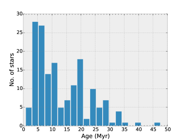
Figure 20: Histogram of ages of the OB stars in the N 206 complex, with bin width of $\sim$2 Myr.

The distribution of ages of all OB stars in our sample is displayed in Fig. 20. It clearly shows multiple peaks across stellar ages, with a maximum in the age range 3-7 Myr. From the HRD we can see that the stars in this age range are mostly O stars and B supergiants. So, massive star formation in the N 206 complex must have peaked in this time period. There are also local maxima at ages 10, 20, and 30 Myr populated by B stars.

We checked our results for correlations between stellar ages and location. Figure  21 shows the position of the OB stars, color-coded with their respective estimated age. For this purpose, we grouped the stars into four different age categories 0-4 Myr, 4-10 Myr, 10-20 Myr, and above 20 Myr, respectively. We can see that the youngest stars are concentrated in the central parts of the complex, especially in the NGC 2018 cluster. Most of the older OB stars are located in the periphery of the N 206 complex.

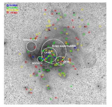
Figure 21: Distribution of the OB stars in the N 206 complex, color-coded with their age

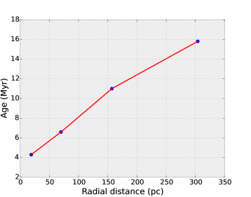
Figure 22: Median age of the OB stars as function of their radial distance from the cluster NGC 2018.

To investigating the variation of ages with location, we divided the region into four annuli with radii of 80, 300, 670, and 1300^′′, respectively, centered at the young cluster NGC 2018. The median of the ages of all OB stars inside each annulus is calculated and plotted in Fig. 22. The radial distances are converted from arc seconds to pc using the LMC distance. Interestingly, we can see a clear trend of the age increasing with distance from the cluster center throughout the whole complex.

We propose two possible explanations for this correlation. One is that the star formation process began in the outer parts. The massive OB stars formed at this time period must have already cleared out their surrounding molecular cloud, and the star formation propagated inwards, where dense molecular gas was left. Another possible scenario is that the star formation happened near the center of the complex, and these stars migrated outward during their lifetime. Given the average radial velocity dispersion of $16\,\rm{km\,s^{-1}}$, a star could travel a projected distance of 240 pc ($\sim$ radius of the complex) in 15 Myr. The dynamical ejection of massive stars from young clusters are also supported by Oh et al. (2015) and Oh & Kroupa (2016).

7.3.4 Mass discrepancy

In Paper I we discussed the mass discrepancy noticed for the Of stars. The same discrepancy is also found here for the whole OB sample. The evolutionary masses of the individual stars are derived from the HRD as described above (see Sect. 7.3). The evolutionary mass (see Table A) represents the current stellar mass of the star as predicted by the track, while the spectroscopic mass (see Table 3) is inferred from $\log\,g$.

In order to check for the discrepancy that we encountered in Paper I, we compared both masses for all OB stars (Fig. 23). We can see a systematic difference between evolutionary and spectroscopic masses, even though the uncertainties are quite high. This mass discrepancy is a well known problem in astrophysics, especially in the case of OB stars in the Magellanic Clouds (McEvoy et al. 2015; Bouret et al. 2013; Massey et al. 2009, 2013). In our sample, the evolutionary masses are systematically lower than the spectroscopic masses. Moreover, the evolved stars (giants and supergiants) show much smaller discrepancies than the main sequence stars. It should be noted that spectroscopic masses have a much higher uncertainty than the evolutionary masses. The one-to-one correlation of the masses falls within this error limit. The study of Galactic B stars by Nieva & Przybilla (2014) gives similar results, where the spectroscopic masses appear to be larger than corresponding evolutionary masses for $M_{\rm spec}>15M_{\odot}$.

Moreover, we cannot rule out the possibility of undetected companion(s) in the spectra, which would also affect the mass determinations. Also we know that a significant fraction of the OB stars in clusters or associations are binaries (Sana et al. 2013a, 2011). Some O stars studied by Bouret et al. (2013) also showed higher spectroscopic than evolutionary masses, and turned out to be binaries. They concluded that the bias toward higher spectroscopic masses is probably related to the binary status of the objects. However, it seems unlikely that all stars in our sample are biased this way.

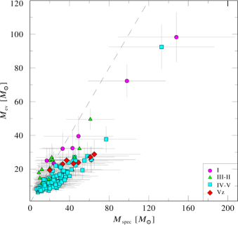
Figure 23: Spectroscopic versus evolutionary masses. The one-to-one correlation of spectroscopic and evolutionary masses is indicated by the dashed line. The sample also includes the Of stars from Paper I. Different luminosity classes are denoted using different shapes and colors as given in the legend.

7.4 Present day mass function

The spectral analysis of hot OB stars in the N 206 region gives a good sample to reveal the present day mass function. Figure 24 (upper panel) shows the present day mass function (PDMF) for the massive stars based on both spectroscopic and evolutionary masses. The corresponding power-law fits give a slope of $\Gamma\approx-2.0$ in both cases. Since the sample becomes incomplete at the lowest masses, the power-law fit is restricted to masses above 20 $M_{\odot}$ in the case of spectroscopic masses, and 10 $M_{\odot}$ for evolutionary masses. It should be noted that the PDMF plotted here might be biased due to unresolved binaries (Weidner et al. 2009). Moreover, the PDMF discussed here is distinct from the initial mass function (IMF), because stars lose mass over their lives, and some disappear after supernova explosions. Since multiple episodes of star formation have occurred in this region, the number of lower mass stars will increase over time and therefore lead to a steeper slope than in the IMF (Kroupa et al. 2013).

In Figure 24 (lower panel) we plot the PDMF only for the young cluster NGC 2018. For this subset of stars, the power-law fit gives a very shallow slope of $\approx 0.9$. This is substantially flatter than the Salpeter slope of the IMF $\Gamma$ = -1.35, and could indicate a top-heavy IMF for this young cluster. In a recent work, Schneider et al. (2018) found a similarly flat IMF for the 30 Doradus starburst in the LMC. Moreover, Marks et al. (2012) deduced a variation of the IMF as becoming top-heavy with decreasing metallicity.

Thus we find a substantial variation of the mass function for different parts of the N 206 complex. To quantify this, we calculate the slopes of the PDMF as a function of distance from NGC 1028. Similar to the analysis in Sect. 7.3.3, we divide the region into four annuli and determine the PDMF for each of the different areas. From the central young cluster to the outer parts of the complex, the slopes are -0.9, -1.4, -1.9, and -2.3, respectively. So, the slope of the PDMF gets gradually steeper with distance from the NGC 2018 cluster. This could indicate mass segregation in the complex. Similar trends are also observed in other clusters like NGC 346 (Sabbi et al. 2008), NGC 3603 (Harayama et al. 2008), and Westerlund 2 (Zeidler et al. 2017).

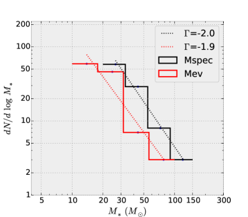
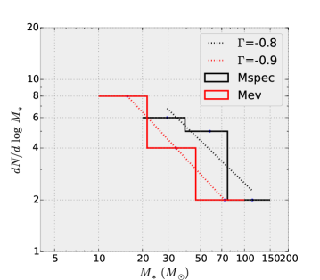
Figure 24: Present day mass function of the whole OB stars in the sample (upper panel) and only for the NGC 2018 cluster (lower panel). The histograms are for spectroscopic (black) and evolutionary (red) masses, respectively. Power laws are fitted to the mass functions (dashed lines) with their slopes $\Gamma$ as given in the legends.

7.5 Present star formation rate

The distribution of stellar ages (Fig. 20) indicates a phase of vivid star formation over the last 7.5 Myr. We extract from our results the spectroscopic masses of all OB stars younger than 7.5 Myr. Together with the two WR binaries, their total mass adds to $2600\,M_{\odot}$. Neglecting the mass lost by winds and SNe, the mass that has been assembled per year into massive stars is thus $2600\,M_{\odot}/7.5\,\mathrm{Myr}=3.6\times 10^{-4}\,M_{\odot}\mathrm{yr}^{-1}$.

Our sample contains the stars with spectroscopic masses above $20\,M_{\odot}$ (see  Fig. 24). For a rough estimate of the mass which went into any stars including those with masses lower than this limit, we adopt a Salpeter IMF and compare the integral from $20$ to $150\,M_{\odot}$ with the integral starting from a lower mass cut-off of $0.5\,M_{\odot}$ (e.g. Kroupa 2002). This calculation indicates a correction factor of about six. Thus, the total star formation rate we obtain is about $2.2\times 10^{-3}\,M_{\odot}\,\mathrm{yr}^{-1}$. This number compares very well with the estimate of $2.5\times 10^{-3}\,M_{\odot}\,\mathrm{yr}^{-1}$ derived from infrared data on young stellar objects, as reported in the Introduction (Sect. 1).

7.6 Stellar feedback in the N 206 complex

We quantify the total stellar feedback of the N 206 complex from our spectroscopic study of its massive star population. The interstellar environment consists roughly of three phases: the cold, neutral, or molecular gas, the ionized H ii regions, and the shock-heated plasma that emits X-rays. Neglecting mutual interactions, the H ii regions are powered by the ionizing radiation of stars, while the X-ray plasma is created by the shocked stellar wind and supernova explosions.

The ionizing photon fluxes generated by the massive stars in our sample will be discussed in Sect. 7.6.1. These ionizing fluxes could be used for constructing photoionization models, and their predictions could be compared with the diffuse emission observed in this complex. In fact, we have placed a number of FLAMES fibers on the diffuse background and plan to do such modeling in the future, but this is beyond the scope of the present paper.

In Sect. 7.6.2, we calculate the total mechanical luminosity produced by the stellar winds of all sample stars as well as the integrated kinetic energy of the winds over the life of the star. In Sect. 7.6.3, we discuss the possible supernova rate in the complex and estimate the input energy. Assuming no interaction between different phases of the ISM, we discuss the energy budget of the superbubble in Sect. 7.6.4 by comparing with the stored energy calculated by Kavanagh et al. (2012).

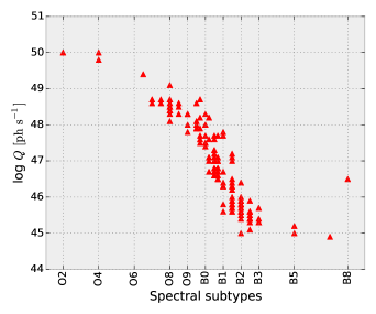
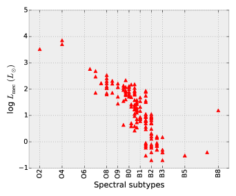
Figure 25: Ionizing photon flux (upper panel) and mechanical luminosity (lower panel) as a function of spectral subtypes.

7.6.1 Ionizing feedback from the WR and OB stars

The rate of hydrogen ionizing photons ($Q_{0}$) for each OB star predicted by their final model is given in the Table. 3. This ionizing photon flux strongly varies with the spectral subtypes of the OB stars as shown in Fig. 25 (upper panel). The present-day total ionizing photon flux produced by all the OB stars in our sample is $Q_{0}\approx 4\times 10^{50}\,\rm{s^{-1}}$. More than 65% of this total ionizing photon flux is contributed by the three very massive Of stars (N206-FS180, 187, and 214). The ionizing photon flux generated by the two WR binaries in the complex is $Q_{0}\approx 5\times 10^{49}\,\rm{s^{-1}}$, which contributes about twelve percent to the combined ionizing feedback from WR and OB stars.

The three Of stars are the only stars in our sample that produce a significant number of He ii ionizing photons. The number rate of such photons with $\lambda<228$ Å is about $\approx 6\times 10^{45}\,\rm{s^{-1}}$.

7.6.2 Mechanical feedback from stellar winds

The mechanical luminosities of the OB stars in the N 206 complex as a function of their spectral subtype are shown in Fig. 25 (lower panel). The total mechanical luminosity generated by all sample OB stars is estimated to be $L_{\rm mec}=\,0.5\,\dot{M}\,\varv_{\infty}^{2}\approx\,2.34\times 10^{4}\,L_{\odot}$. Similar to the ionizing photon flux, the total mechanical luminosity is also dominated ($\sim$62%) by the three very massive Of stars.

Since we know the ages (see Sect. 7.3.3) and the mechanical luminosity (see Table 3) of the individual OB stars, we can construct a diagram for the evolution of the mechanical luminosity in the entire complex with time (see Fig. 26). The red line illustrates the total mechanical luminosity of all OB stars at a particular time. Here we assume that all our sample OB stars had a constant mechanical output since their formation. Since most of our sample OB stars are still in their hydrogen burning phase (before reaching the terminal age main sequence) as evident from the HRD, this assumption is justified for a rough estimate. Therefore, if only accounting for those OB stars which still exist today, the total mechanical luminosity would have increased over the past five Myr. Of course, this curve might change a lot due to previous generations of massive stars which are no longer present today.

In order to calculate the total mechanical energy released by all presently existing OB stars via stellar winds throughout their life, we must integrate their mechanical luminosity over their age. We obtained a total mechanical feedback from our sample OB stars of $E_{\rm mec}=\,0.5\,\dot{M}\,\varv_{\infty}^{2}t\,\approx 1.1\times 10^{52}\,\rm{erg}$. Even if we are considering only the past five Myr, the accumulated mechanical feedback is $E_{\rm{mec}}\approx 9.5\times 10^{51}\,\rm{erg}$. However, these estimates of mechanical feedback only consider those massive stars that are still present in the N 206 complex today, and does not account for those massive stars which have already disappeared. Therefore, these estimates are only lower limits to the stellar wind feedback.

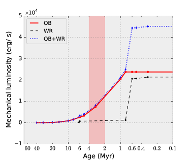
Figure 26: Evolution of the mechanical luminosity in the N206  complex, only considering the present stellar content. The mechanical luminosity from WR and OB stars is shown in black dashed and red solid lines, respectively. The combined mechanical luminosity is represented by the blue dotted line. The red shaded area indicates the time interval in which the superbubble formation has begun.

Table 6: Feedback from the WR binaries

		N206-FS45	N206-FS128
pre-WR phase	$\log\dot{M}$ [$M_{\odot}\,\mathrm{yr}^{-1}$]	-6.5	-6.1
	$\varv_{\infty}$ [km s-1]	2600	2800
	$L_{\rm mec}$ [$L_{\odot}$]	177	514
	$t$ [Myr]	6.2	5.4
	$E_{\rm mec}$ [$10^{50}$erg]	1.3	3.3
WR phase	$\log\dot{M}$ [$M_{\odot}\,\mathrm{yr}^{-1}$]	-5.4	-4.67
	$\varv_{\infty}$ [km s-1]	1700	3400
	$L_{\rm mec}$ [$L_{\odot}$]	950	20400
	$t$ [Myr]	0.3	0.6
	$E_{\rm mec}$ [$10^{50}$erg]	0.34	14.75

The WR stars make a significant contribution to the mechanical feedback of the region. Here we only discuss the feedback from the primary (WR) component, since the contribution from the secondary component (late O star) is comparatively much smaller. The details of the feedback parameters of the WR stars N206-FS 45 and 128 are given in Table 6.

The evolutionary tracks predict (see Sect. 7.3.2) the initial parameters of the star N206-FS 128a at the ZAMS as $T_{\ast}=39$ kK, $\log\,g_{\ast}=4.1$, $\log\,(L/L_{\odot})=5.2$, $\log\dot{M}\sim-6.1\,[M_{\odot}$ yr${}^{-1}]$, and $\varv_{\infty}\sim 2800$ km s^-1. Here, $\varv_{\infty}$ is calculated theoretically from $\varv_{\rm esc}$. The mechanical energy produced by this star is about $3.3\times 10^{50}\,\rm{erg}$ over the first 5.4 Myr. The star then stayed in the WR stage for the last 0.6 Myr, imparting a wind energy of approximately $1.5\times 10^{51}\,\rm{erg}$ to the surroundings. Thus, the mechanical feedback from N206-FS 128 throughout its life is $E_{\rm mec}\approx 1.8\times 10^{51}\,\rm{erg}$.

The feedback contribution from the WN component of the binary N206-FS 45 has been estimated by Shenar et al. (in prep.) on the basis of a spectral analysis. The current period of the system is 36.9 days (Foellmi et al. 2003). For the derived parameters (see Table 4), the binary evolutionary tracks by Eldridge & Stanway (2009) suggest an age of $\approx$ 6.5 Myr and an initial mass of the WN component of $30\,M_{\odot}$. The star spent $\approx$ 6.2 Myr in the hydrogen burning phase. The mechanical luminosity estimated for this time period is $\approx 177\,L_{\odot}$, and the integrated mechanical energy amounts to $E_{\rm{mec}}\approx 1.3\times 10^{50}\,\rm{erg}$. The star has stayed in the WR stage over the last 0.3 Myr. The mechanical energy released by the WR wind during this time period is $\approx 3.4\times 10^{49}\,\rm{erg}$. Therefore, the model predicts the accumulated mechanical energy output of this star in both stages to be $E_{\rm{mec}}\approx 1.6\times 10^{50}\,\rm{erg}$.

Table 6 summarizes the feedback from N206-FS 45 and N206-FS 128 in both the pre-WR and WR phase. Now we add these contributions to the mechanical luminosity over time plotted in (Fig. 26). From the diagram, we can see that the two WR stars contribute to the feedback about as much as the whole sample of hundreds of OB stars. The total mechanical luminosity is about $L_{\rm{mec}}=4.5\times 10^{4}\,L_{\odot}=1.7\times 10^{38}\,\rm{erg\,s^{-1}}$.

The integrated mechanical energy over the lifetime of both WR stars in our sample is $\approx 2\times 10^{51}\,\rm{erg}$. So, the total accumulated mechanical feedback over the lifetimes of the current WR and OB stars becomes $E_{\rm{mec}}\approx 1.3\times 10^{52}\,\rm{erg}$. Even if we consider only the past five Myr, the total integrated mechanical feedback is $\approx 1.2\times 10^{52}\,\rm{erg}$.

From the size and expansion velocity of the X-ray superbubble, Dunne et al. (2001) suggest an age of $\sim$2 Myr. According to Kavanagh et al. (2012), the expansion of the superbubble must have undergone induced acceleration in its history, and therefore it is likely to be older than 2 Myr. The HRD of the stars in the X-ray superbubble region (Fig. 17, lower right) reveals many O stars within the age range $4-5$ Myr. Therefore we speculate that the age of the superbubble is about $2-4$ Myr. This time interval is marked in Fig. 26 by a shaded area. As seen in Fig. 20, the star formation in the N 206 complex peaked $3-5$ Myr ago. In this period, the stellar winds from this population must have caused a rapid increase in the overall mechanical luminosity.

Regarding the times more than five Myr ago, it should be noted that we are not aware of the full star formation history. There might have been other time intervals of peak star formation. However, considering only the present stellar content, $L_{\rm{mec}}$ was negligible before 5 Myr, then it started to grow and led to the formation of the superbubble. The huge increase in $L_{\rm{mec}}$ over the last 0.6 Myr is due to the two WR stars.

7.6.3 Feedback from supernovae

A single supernova (SN) injects typically $10^{51}$ erg of mechanical energy into the ISM (Woosley & Weaver 1995). Therefore, for our study we need to estimate the number of supernovae that have already occurred in the N 206 complex.

Currently, there is only one SNR situated in this complex, which suggests that a SN that occurred within the last few ten thousand years. Older SNRs would have already faded below the observational limit.

Indirect evidence for previous SNe could come from the detection of X-ray binaries. The formation of their compact component, a black hole or neutron star, might have been accompanied by a SN explosion. Previous studies by Shtykovskiy & Gilfanov (2005) and Kavanagh et al. (2012) have identified two HMXB candidates, namely XMMU J052952.9-705850 and USNO-B1.0 0189-00079195, by the X-ray analysis of the region using XMM-Newton telescope data. In order to check the nature of these objects, we have taken VLT-FLAMES spectra at the positions of both X-ray sources (Fig. 27). In both cases, no stellar features can be detected, neither lines nor a continuum. The data show only nebular emission from the diffuse background in both cases. Hence we do not support the identification of these X-ray sources with HMXBs. Our conclusion is supported by the Million Optical - Radio/X-ray Associations (MORX) Catalog (Flesch 2016), which also suggests that these X-ray sources are most probably contaminations from background quasars or external galaxies.

Further indirect evidence for previous SN occurrences is given by OB runaways. These stars might have been ejected from a binary system, when the SN explosion of the primary disrupted the system. In Sect. 7.1 we identified eight runaway candidates with radial velocities in excess of $\pm$48 km s^-1. Interestingly, most of these stars are located inside or at the periphery of the X-ray superbubble as shown in Fig. 12.

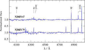
Figure 27: Normalized VLT-FLAMES LR02+LR03 spectra taken at the positions of the X-ray sources XMMU J052952.9-705850 (upper panel) and USNO-B1.0 0189-00079195 (lower panel)

Considering the evolutionary masses of the OB stars, there are about 36 stars in the $20-40\,M_{\odot}$ bins and five stars with masses $\geq 40\,M_{\odot}$, which must become SNe within the next ten and five Myr, respectively. Additionally, there are two WR binaries in the complex. These numbers are higher than predicted by Kavanagh et al. (2012) from the IMF. If the SFR was roughly constant in time, there should have been a similar number of massive stars in the past.

In Ferrand & Marcowith (2010), the rate of supernovae in massive clusters or OB associations is expressed to first approximation as

$$\frac{{\rm d}n}{{\rm d}t_{\rm SN}}\approx\frac{N_{*}}{\Delta t^{*}_{\rm OB}}.$$ (2)

Here $\Delta t^{*}_{\rm OB}=t_{\rm SN}(m_{\rm min})-t_{\rm SN}(m_{\rm max})$ is the active lifetime of the cluster, where $m_{\rm min}$ and $m_{\rm max}$ are the minimum and maximum initial mass of the stars in the region that explode as SNe. The symbol $N_{*}$ is the number of stars with masses between $m_{\rm min}$ and $m_{\rm max}$. Regarding the SN rate in the N 206 complex, we can take $m_{\rm min}=8\,M_{\odot}$ and $m_{\rm max}=100\,M_{\odot}$. This gives $t_{\rm SN}(m_{\rm min})\approx 37$ Myr and $t_{\rm SN}(m_{\rm max})\approx 3.5$ Myr. From the HRD, 162 stars have $M_{\rm ini}\geq 8\,M_{\odot}$ (including binary companions). So, the supernova rate is $\approx$ 4.8 per Myr or one SN per 210,000 years. Even if we consider only stars with initial masses below $40\,M_{\odot}$, because more massive stars might collapse silently (Heger et al. 2003), the rate is $\approx$ five supernovae per Myr. This number is in statistical agreement with the presence of just one SNR today.

If we do the same calculation only for massive stars within or close to the X-ray superbubble (including stars in NGC 2018, LH 66, and LH 69), the estimated SN rate is $\approx$2.2 per Myr. So, if we consider only the past five Myr and massive stars close to the X-ray superbubble, the accumulated mechanical input by supernova explosions is estimated to be $E_{\rm{mec}}\approx 1.1\times 10^{52}\,\rm{erg}$, and hence contributes approximately the same amount to the mechanical feedback as the massive star winds.

7.6.4 Superbubble energy budget

We compare our energy feedback results with the X-ray analysis of the superbubble by Kavanagh et al. (2012). Using XMM-Newton data, they estimated the X-ray luminosity of the N 206 superbubble as $\approx 7\times 10^{35}$ erg s^-1. In young star clusters, the unresolved X-ray emission from the population of active pre-main sequence stars could be significant (Nayakshin & Sunyaev 2005; Wang et al. 2006), also at sub-solar metallicities (Oskinova et al. 2013). Kavanagh et al. (2012) estimated the contribution from the unresolved low-mass population to the observed X-ray emission as $\sim 6$%. Moreover, the distribution of YSO candidates (Carlson et al. 2012) shows that they are not concentrated in the X-ray superbubble area.

To estimate the contribution of young active stars of low mass to the extended X-ray emission in N 206, we use the scaling provided in Oskinova (2005). Their figure 5 compares the relative contributions to the X-ray emission from the hot cluster wind with the emission from the unresolved population of low-mass stars. As can be seen in this figure, in clusters younger than $\sim 2.5$ Myr (assuming an instantaneous burst of star formation), the collective X-ray luminosity of low-mass stars dominates the cluster X-ray luminosity. However, for older clusters, the input of mechanical energy from massive stars dominantly powers the diffuse X-ray emission. We estimated the age of the X-ray superbubble in N 206 as higher than 2 Myr (see Fig. 26). Moreover, we found that star formation has been ongoing in this region for a longer time. Hence, it is most likely that the observed soft diffuse X-ray emission is dominated by the mechanical energy input from massive stars.

The observed X-ray luminosity is only 0.4% of the combined mechanical luminosity of the WR and OB stellar winds (see Sect. 7.6.2). The uncertainty in $L_{\rm{mec}}$ is about 30% reflecting the error margins of the stellar wind parameters ($\dot{M},\varv_{\infty}$). Previous studies on other massive star forming regions such as the Omega Nebula, the Rosette Nebula (Townsley et al. 2003), 30 Doradus (Lopez et al. 2010; Doran et al. 2013), and the Carina Nebula (Smith 2006; Townsley et al. 2011) also revealed similar trends, where only a small portion of the wind energy is converted into X-ray emission. Rosen et al. (2014) published a detailed study about missing stellar wind energy from massive star clusters. They suggest that turbulent mixing at the hot-cold interface or physical leakage of the shock heated gas can efficiently remove the kinetic energy injected by the massive star winds and supernovae.

Kavanagh et al. (2012) also estimated the total energy stored in the superbubble in the form of thermal energy of the shock-heated gas and the kinetic energies of the expanding H$\alpha$ and H i shells to be $(4.7\pm 1.3)\,\times 10^{51}$ erg. The feedback calculations discussed in the previous sections reveal a much higher mechanical energy input by the massive stars to the N 206 complex. Adding the mechanical energy input during the last five Myr from the OB and WR star winds (Sect. 7.6.2) and the SNe (Sect. 7.6.3), we obtain $\approx 2.3\times 10^{52}$ erg, which is almost five times higher than the stored energy content observed by Kavanagh et al. (2012). Even more, the feedback estimates are only a lower limit, as discussed in Sect. 7.6.2. With the SN rate estimated in Sect. 7.6.3, about 25 supernovae might have occurred in the entire complex during the past five Myr. Also, there would be a contribution from stellar winds of their progenitors. Considering these numbers, the total $E_{\rm{mec}}$ can increase by a factor of roughly two. However, this does not include the contribution from stars which already died as SNe between 5 to 50 Myr ago (Fig. 26). According to the SNe estimation given in Sect. 7.6.3, about 250 stars might have already exploded as SNe. Here we assumed a constant star formation rate over the past 50 Myr, as high as the current rate. During their evolutionary stages, stellar winds (OB/WR) of these stars would have provided a significant amount of mechanical feedback. Supernovae and stellar winds together might have released about 15 times more mechanical energy than our estimated value of $2.3\times 10^{52}$ erg. As we have seen above, the radiative cooling by X-ray emission is negligible. Hence, this comparison shows that most of the mechanical energy input has been consumed by other processes or escaped from the X-ray superbubble.

The hot X-ray emitting gas could not escape, if it were fully confined by surrounding cold and dense molecular material. Figure 28 shows a multiwavelength image of the N 206 complex at far-infrared, optical, and X-ray wavelengths, over-plotted with CO intensity contours. The CO intensity map taken from the Magellanic Mopra Assessment (MAGMA) (Wong et al. 2011) traces the dense molecular gas. This map reveals that the X-ray superbubble is only partially confined by the dense molecular cloud. In the 2D projection, it seems that the X-ray emitting gas leaks out in northern directions. Figure 28 also gives a general picture of ongoing star formation in this region. When comparing this with Fig. 21, we can see that now the star formation is presently progressing at the rim of the cloud. This could be an indication of a triggered star formation in the complex by the expansion of the superbubble when it hits the rim of the cloud. The young cluster NGC 2018 is also located in this dense part of the molecular cloud. At the other side of the superbubble, the cold molecular gas is already removed, which might be due to the energetic winds of massive stars or SNe that occurred in the past. So, mostly older stars are left there, and there is not enough material available for further star formation.

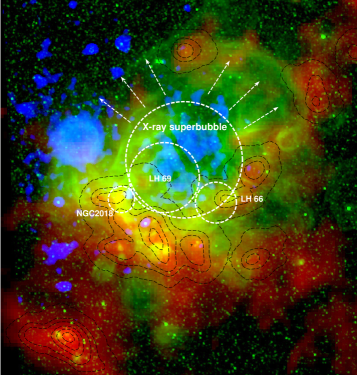
Figure 28: Color composite image of the N 206 complex, constructed from the Herschel spire data (red: 500 $\mu m$), H$\alpha$ (green: MCELS, Smith et al. 2005), and X-rays (blue: XMM-Newton $0.3-1$ keV). CO intensity contours taken from the MAGMA survey are over-plotted to the image. The arrows suggest the possible leakage of hot gas from the X-ray superbubble.

8 Summary and conclusions

We have identified and analyzed the OB stars and WR binaries in the N 206 complex located in the LMC. The stellar and wind parameters of the individual stars are determined using PoWR model atmospheres. We also present a detailed binary analysis of the WC4+O9 system, and discuss its evolutionary status. Our main conclusions are:

• Approximately 12% of the whole sample are found to be emission-line stars with a disk. However, our analysis shows that the projected rotational velocities of most of these Oe/Be stars are far below their critical velocity.

• From the radial velocity distribution of the OB stars, we suspect eight stars to be runaways.

• The wind momentum-luminosity relation of most of the sample OB stars is consistent with expectations within uncertainties.

• The HRD of our OB star sample in the complex reveals multiple populations of different ages. Moreover, each of the clusters and OB associations inside the region also shows large age dispersions, indicating multiple star formation events.

• The current stellar masses as derived from evolutionary tracks are systematically lower than the masses that we obtain from our spectroscopic analyses. This discrepancy is higher for main sequence stars than for evolved stars.

• We find indications of sequential star formation in the region. The youngest stars are mostly distributed inside the young clusters and the inner part of the complex, whereas outer parts contain slightly older populations.

• The current star formation is taking place at the rim of the superbubble, where it hits the molecular cloud.

• The present day mass function of the entire region shows a steeper slope than the Salpeter IMF. However, the cluster NGC 2018 shows a top-heavy mass function.

• We derive the current star formation rate of the complex as $2.2\times 10^{-3}M_{\odot}\,\mathrm{yr}^{-1}$.

• The total ionizing photon flux produced by all massive stars in the N 206 complex is $Q_{0}\approx 5\times 10^{50}\,\rm{s^{-1}}$.

• Three very massive Of stars out of 164 OB stars contribute $>$60% of the total ionizing photon flux and the stellar wind mechanical luminosity.

• The integrated mechanical energy feedback from all OB stars over the past five Myr is estimated to be $\approx 1.3\times 10^{52}\,\rm{erg}$. This is more than the energy that is found to be stored in the superbubble.

• The two WR binaries contribute about as much mechanical luminosity as all the 164 OB stars in the sample.

• The rate of supernova explosions in the complex is estimated to be about five per Myr.

• The X-ray luminosity of the N 206 superbubble is only 0.4% of the current mechanical luminosity from the stellar winds of the OB + WR stars.

• The energy input accumulated over time from the OB stars, WR stars, and SNe is found to be more than five times higher than the energy stored in the X-ray superbubble.

• The morphology of the complex, with the X-ray superbubble not being fully enclosed by the cold molecular gas, gives the impression that the hot gas has the possibility to escape from the complex.

• The fact that a few of the most massive stars dominate the energetics of the N 206 complex would not have been revealed without spectroscopic information.

Appendix A Additional tables

Table 7: Coordinates and spectral types of OB stars in our sample (continuation of Table 1)

N206-FS	RA (J2000)	DEC (J2000)	Spectral type
#	(°)	(°)
31	82.307375	-70.865306	B3 IV
32	82.325375	-71.218750	B0 V
33	82.331500	-71.029611	B8 Ia
34	82.337333	-71.029389	B1.5 III Nwk
36	82.346625	-71.082000	B2 IV
37	82.348583	-71.092639	B1.5 IV
38	82.350667	-71.074139	B2 V
39	82.365375	-71.073444	B1.5 V
42	82.374917	-70.901500	B2 IV
43	82.384500	-70.992333	B0.5 V
46	82.399375	-70.937000	B1.5 V
47	82.408458	-70.963778	O9.7 V
48	82.409125	-70.990472	B0.7 V
49	82.411208	-70.985083	B1.5 V
50	82.412125	-70.985778	B1 V
51	82.412458	-70.982944	B2 IV
52	82.429292	-70.837722	B0 V
55	82.436708	-70.916278	B0.2 IV
56	82.438917	-71.161500	B0.7 (IV)e
58	82.442250	-71.156111	B0.5 II
60	82.446917	-71.150111	B1.5 (IV)e
61	82.455208	-71.063139	B1.5 V
62	82.462500	-71.105500	O9.5 (III)e
64	82.464958	-71.075722	O8 Vz
65	82.465500	-71.068611	B2 IV
68	82.471250	-71.083889	B2.5 IV
69	82.471583	-71.079000	B0.2 V
73	82.479625	-71.149639	B0.7 IV
74	82.494250	-70.931778	B0.5 V
75	82.496542	-71.099333	B0.7 IV
77	82.497500	-70.848306	B0.5 V
78	82.503083	-71.160111	B1 V
80	82.510292	-71.088917	B1.5 V
81	82.517667	-71.132278	B1 II
84	82.523792	-71.152778	B1.5 IV
88	82.528583	-70.829889	B0 V
89	82.544917	-71.079056	B2 IV
90	82.546875	-70.861667	O9.7 Iab
91	82.546958	-71.079583	O8 IV
93	82.548625	-71.099917	B0.2 V
95	82.549083	-71.067472	B0.5 IV
98	82.567542	-71.104611	B0.7 IV
99	82.581125	-71.102000	O9.5 V
101	82.582333	-71.280056	B1.5 (IV)e
103	82.589083	-70.813639	B2 (IV)e
104	82.592167	-70.910028	B0.5 V
105	82.592250	-71.105389	B1.5 V
107	82.594583	-71.105417	O8 Vz
108	82.594708	-71.099611	B1.5 V
109	82.596000	-71.056639	B0.5 V
112	82.609125	-70.983639	O9.7 V
113	82.613167	-71.048917	B3 (V)e
116	82.617792	-70.989889	B0.7 III
117	82.625625	-70.890972	B2 (IV)e
119	82.627875	-71.042083	O8 (V)e
120	82.636708	-71.049361	B2 IV
121	82.640458	-70.831000	B1.5 (V)e
122	82.646792	-71.032472	B1.5 (IV)e
123	82.647833	-71.081194	B0.2 V
125	82.652583	-71.071000	O9 V
126	82.653000	-71.028583	B2 V
127	82.659750	-71.085278	B0.2 V
129	82.663083	-71.016611	B0.5 IV
130	82.664750	-71.055778	O9.7 V
132	82.666750	-71.286972	O9 IV
133	82.667125	-71.113139	O9 V
134	82.667250	-71.093611	O9.7 Iab
136	82.674125	-70.892889	B1 V
138	82.685458	-71.029000	B0.7 V
139	82.691667	-70.874306	B0.7 V
141	82.693083	-70.866500	B1.5 V
142	82.693750	-70.895667	B2 (V)e
143	82.694000	-70.913778	B1.5 V
144	82.696042	-71.054333	B0 II Nwk
145	82.697958	-71.133667	O8 Vz
146	82.697958	-71.058083	B1.5 IV
147	82.699083	-71.067278	B1 Ia Nwk
148	82.701792	-71.230222	O9.7 IV
149	82.703083	-71.065917	O9 IV
150	82.706750	-71.004278	B0.5 V
151	82.710958	-71.046639	O7.5 V
153	82.714833	-71.216167	B2 IV
154	82.723083	-71.132889	O7 Vz
155	82.724667	-71.064833	B0.7 V
156	82.726875	-71.086278	B0.2 I
157	82.728917	-70.895361	B2 V
159	82.734792	-70.915111	B2 V
160	82.734917	-71.072167	B0 II Nwk
163	82.740167	-71.025389	B0.5 III
164	82.747125	-71.072389	B1.5 V
165	82.748792	-70.958750	B3 V
167	82.750750	-70.810028	B5 V
168	82.753417	-71.077389	B2 V
170	82.762250	-70.832333	B1 IV
172	82.778292	-71.179861	O8.5 V
173	82.782458	-71.130361	O9.7 V
174	82.783083	-71.129889	O9.7 V
175	82.784208	-71.028500	B0 III
176	82.788292	-71.070694	O8.5 V
177	82.789958	-71.064306	B2 V
179	82.796833	-71.158167	B1 V
181	82.799750	-71.081639	B1.5 (III)e
183	82.804833	-71.073722	B0.5 V
184	82.807750	-71.064167	O8 Vz
185	82.810333	-71.068875	B2 V
186	82.813100	-71.069500	O9 (V)e
189	82.816125	-71.167472	B2.5 V
190	82.824708	-71.107389	B2 V
191	82.825125	-71.067111	B0.5 V
192	82.828458	-71.077500	O9.5 (III)e
194	82.848833	-71.070194	O8.5 V
195	82.851708	-70.934694	B0.7 V
196	82.852250	-71.139750	B0.2 IV
197	82.852792	-71.064139	B0 V
198	82.852833	-71.070889	O8 Vz
200	82.892125	-70.940389	B1.5 IV
201	82.892458	-71.160556	B0.5 V
202	82.892583	-70.951361	B2 V
204	82.900333	-71.115917	B2.5 V
205	82.910917	-70.959972	B1.5 V
206	82.915042	-70.963417	B2 V
207	82.916000	-71.111972	B2.5 V
209	82.921000	-70.961556	B0.7 V
211	82.925333	-71.008500	B1 V
213	82.948583	-71.151278	B3 V
215	82.957792	-70.964722	B0 IV
220	82.993000	-70.962694	B3 IV
221	82.994625	-71.253000	B3 V
222	82.996583	-71.161722	B1.5 IV
224	83.000167	-71.235472	B2 III
225	83.012833	-71.053778	B2.5 V
229	83.036750	-71.032778	O9.5 V
231	83.067583	-71.234000	B2 V
232	83.076792	-71.088139	B2.5 V
233	83.145083	-71.113722	B1.5 (V)e
234	83.174125	-71.045583	B0.5 (V)e

Table 8: Stellar parameters of all OB stars in the N 206 superbubble (continuation of Table 3)

N206-FS	Spectral type	$T_{\ast}$	log $L$	log $g_{\ast}$	log $\dot{M}$	$E_{B-V}$	$M_{\mathrm{V}}$	$R_{\ast}$	$\varv_{\infty}$	$\varv$ sin $i$	$\varv_{\rm rad}$	$M_{\ast}$	$\log Q_{0}$	$L_{\mathrm{mec}}$
#		[kK]	[$L_{\odot}$]	[cm s-2]	[$M_{\odot}\,\mathrm{yr}^{-1}$]	[mag]	[mag]	[$R_{\odot}$]	[km s-1]	[km s-1]	[km s-1]	[$M_{\odot}$]	[s-1]	[$L_{\odot}$]
31	B3 IV	18.0	3.83	3.6	-8.07	0.12	-3.03	8.5	800	90	290	10	45.3	0.4
32	B0 V	31.0	4.53	4.2	-6.85	0.15	-3.18	6.4	2400	150	260	24	47.5	67.1
33	B8 Ia	13.5	5.30	2.0	-6.28	0.12	-7.19	81.9	600	65	270	24	46.5	15.68
34	B1.5 III Nwk	23.0	4.80	3.4	-7.70	0.12	-5.08	15.9	1500	80	220	23	47.0	3.7
36	B2 IV	20.0	4.03	3.6	-7.93	0.15	-3.29	8.6	800	150	260	11	45.6	0.6
37	B1.5 IV	20.0	4.20	3.4	-8.00	0.12	-3.76	10.5	600	130	260	10	45.7	0.3
38	B2 V	19.0	4.00	3.8	-7.70	0.10	-3.47	9.3	1000	100	260	20	45.6	1.6
39	B1.5 V	22.0	4.17	4.0	-7.62	0.12	-3.16	8.4	2400	160	240	26	45.9	11.3
42	B2 IV	20.0	4.03	4.0	-7.35	0.12	-3.51	8.6	1200	180	250	27	45.9	5.3
43	B0.5 V	27.0	4.26	4.2	-6.78	0.10	-3.03	6.2	2500	75	240	22	46.7	86.6
46	B1.5 V	25.0	4.11	4.2	-7.24	0.11	-2.93	6.1	2600	100	260	21	46.3	32.3
47	O9.7 V	31.0	4.87	4.0	-6.78	0.07	-4.39	9.5	2200	264	240	33	47.9	67.0
48	B0.7 V	27.0	4.40	4.0	-7.45	0.10	-3.78	7.3	2100	100	180	19	47.0	12.9
49	B1.5 V	22.0	3.97	4.0	-7.78	0.08	-2.97	6.7	2100	80	240	16	45.6	6.1
50	B1 V	25.0	4.06	4.2	-7.78	0.08	-3.12	5.7	2500	100	250	19	46.3	8.7
51	B2 IV	21.0	4.20	3.8	-7.70	0.05	-3.71	9.5	2000	245	240	21	45.8	6.6
52	B0 V	31.0	4.53	4.2	-6.85	0.08	-3.68	6.4	2400	35	240	24	47.5	67.1
55	B0.2 IV	30.0	5.24	3.8	-6.43	0.12	-5.05	15.5	2200	110	270	55	48.2	150.1
56	B0.7 (IV)e	27.0	4.50	4.0	-7.38	0.22	-3.35	8.1	2200	188	260	24	47.1	16.8
58	B0.5 II	25.0	5.05	3.0	-7.95	0.20	-5.34	17.9	1700	100	240	12	47.7	2.69
60	B1.5 (IV)e	19.0	4.49	3.4	-7.90	0.23	-4.07	16.3	760	86	240	24	46.2	0.6
61	B1.5 V	24.0	3.95	4.2	-7.78	0.03	-2.82	5.5	2500	120	180	17	46.0	8.7
62	O9.5 (III)e	30.0	4.85	3.4	-7.07	0.18	-3.97	9.9	800	383	260	9	48.1	4.4
64	O8 Vz	35.0	5.06	4.2	-6.50	0.09	-4.65	9.2	2800	100	240	49	48.5	204.6
65	B2 IV	20.0	3.85	3.8	-8.54	0.10	-2.88	7.0	900	100	260	11	45.0	0.2
68	B2.5 IV	19.0	3.90	3.8	-7.78	0.10	-2.94	8.2	1000	80	230	16	45.5	1.4
69	B0.2 V	27.0	4.26	4.2	-7.38	0.09	-3.07	6.2	2500	150	210	22	46.7	21.7
73	B0.7 IV	27.0	4.60	4.0	-7.70	0.12	-3.89	9.1	2100	70	240	31	47.0	7.3
74	B0.5 V	29.0	4.64	4.2	-6.62	0.12	-3.80	8.3	2800	100	240	40	47.3	153.4
75	B0.7 IV	25.0	4.55	3.8	-7.78	0.15	-4.06	10.1	2000	150	250	23	46.8	5.5
77	B0.5 V	27.0	4.19	4.2	-7.43	0.07	-2.99	5.7	2400	150	240	19	46.6	17.8
78	B1 V	25.0	4.16	4.2	-7.20	0.08	-3.07	6.4	2600	80	240	24	46.3	35.2
80	B1.5 V	21.0	4.10	3.8	-7.78	0.12	-3.33	8.5	1900	100	220	17	45.7	5.0
81	B1 II	23.0	5.34	2.8	-5.95	0.12	-6.06	29.5	400	87	160	20	47.8	14.9
84	B1.5 IV	22.0	4.12	4.0	-7.66	0.14	-3.44	7.9	2300	218	230	23	45.8	9.5
88	B0 V	30.0	4.64	4.2	-6.70	0.06	-4.08	7.8	2700	70	260	35	47.5	120.0
89	B2 IV	22.0	4.07	4.0	-7.70	0.12	-3.07	7.5	2300	130	260	20	45.8	8.7
90	O9.7 Iab	30.0	5.53	3.4	-6.86	0.12	-5.86	21.6	1891	90	260	43	48.7	40.9
91	O8 IV	34.0	5.16	4.0	-6.75	0.26	-4.31	11.0	2200	274	260	44	48.5	70.6
93	B0.2 V	29.0	4.96	4.0	-7.78	0.21	-4.60	12.0	1700	80	240	53	47.6	3.98
95	B0.5 IV	28.0	4.95	3.8	-6.70	0.12	-4.80	12.7	2000	80	260	37	47.6	65.9
98	B0.7 IV	27.0	4.39	4.2	-7.28	0.03	-3.65	7.2	2700	100	250	30	46.8	31.7
99	O9.5 V	32.0	4.77	4.2	-6.73	0.20	-3.50	7.9	2700	150	240	36	47.9	112.0
101	B1.5 (IV)e	20.0	4.18	3.6	-7.81	0.24	-3.30	10.3	800	232	230	15	45.7	0.8
103	B2 (IV)e	21.0	4.10	3.8	-7.78	0.16	-3.41	8.5	1900	150	280	17	45.7	5.0
104	B0.5 V	27.0	4.50	4.0	-7.38	0.04	-3.72	8.1	2200	200	230	24	47.1	16.8
105	B1.5 V	22.0	4.07	4.0	-7.70	0.12	-3.00	7.5	2300	100	240	20	45.8	8.7
107	O8 Vz	34.0	5.03	4.0	-6.45	0.14	-4.39	9.5	2100	40	250	33	48.4	129.1
108	B1.5 V	22.0	3.97	4.0	-7.78	0.10	-2.99	6.7	2200	140	240	16	45.7	6.7
109	B0.5 V	27.0	4.36	4.2	-6.70	0.15	-3.10	6.9	2600	90	250	28	46.8	111.3
112	O9.7 V	31.0	4.58	4.2	-6.81	0.08	-3.68	6.8	2500	390	260	27	47.5	79.4
113	B3 (V)e	18.0	4.28	3.6	-7.74	0.20	-3.51	14.2	1000	230	240	29	45.7	1.5
116	B0.7 III	25.0	5.08	3.0	-6.78	0.12	-5.27	18.5	1200	252	260	13	47.7	19.83
117	B2 (IV)e	20.0	4.18	3.6	-7.81	0.16	-3.73	10.3	800	72	260	15	45.7	0.8
119	O8 (V)e	34.0	5.28	4.0	-6.66	0.17	-5.10	12.6	2470	100	240	58	48.7	110.78
120	B2 IV	20.0	4.03	3.6	-7.93	0.08	-3.32	8.6	800	110	250	11	45.6	0.6
121	B1.5 (V)e	21.0	4.16	3.8	-7.73	0.23	-3.42	9.1	2000	140	260	19	45.8	6.1
122	B1.5 (IV)e	26.0	4.80	3.8	-6.66	0.28	-4.44	12.4	2100	140	240	36	47.2	79.2
123	B0.2 V	28.0	4.49	4.0	-7.85	0.10	-3.49	7.5	2100	90	240	20	47.1	5.1
125	O9 V	34.0	4.98	4.2	-6.70	0.13	-4.38	8.9	2700	160	290	46	48.3	120.0
126	B2 V	21.0	4.20	3.8	-7.70	0.03	-3.76	9.5	2000	251	230	21	45.8	6.6
127	B0.2 V	28.0	4.39	4.0	-7.93	0.10	-3.23	6.7	2000	80	260	16	47.0	3.9
129	B0.5 IV	28.0	4.69	4.0	-7.70	0.10	-4.22	9.4	2400	110	200	32	47.3	9.5
130	O9.7 V	31.0	4.63	4.2	-6.78	0.07	-3.67	7.2	2500	80	260	30	47.6	86.6
132	O9 IV	32.0	5.03	3.8	-6.93	0.12	-4.61	10.7	1700	160	260	26	48.3	28.3
133	O9 V	34.0	4.98	4.2	-6.70	0.40	-3.91	8.9	2700	110	260	46	48.3	120.0
134	O9.7 Iab	30.0	5.50	3.4	-6.09	0.16	-6.22	20.9	1800	90	260	40	48.7	218.58
136	B1 V	23.0	4.07	4.0	-7.70	0.07	-2.84	6.8	2200	180	250	17	45.8	8.0
138	B0.7 V	26.0	4.16	4.2	-7.28	0.05	-2.75	5.9	2500	140	260	20	46.5	27.4
139	B0.7 V	26.0	4.16	4.2	-7.28	0.08	-3.02	5.9	2500	110	250	20	46.5	27.4
141	B1.5 V	23.0	3.94	4.2	-7.70	0.06	-2.74	5.9	2600	80	240	20	46.2	11.1
142	B2 (V)e	21.0	4.20	3.8	-7.70	0.14	-3.72	9.5	2000	120	240	21	45.8	6.6
143	B1.5 V	22.0	3.97	4.0	-7.78	0.10	-3.18	6.7	2200	120	270	16	45.7	6.7
144	B0 II Nwk	26.0	5.39	3.0	-6.55	0.25	-5.84	24.5	1585	75	320	22	48.3	58.76
145	O8 Vz	35.0	5.16	4.2	-6.43	0.18	-4.97	10.4	2900	120	250	62	48.6	260.8
146	B1.5 IV	23.0	4.18	3.8	-8.49	0.10	-3.36	7.8	1800	120	220	14	46.3	0.9
147	B1 Ia Nwk	20.0	5.78	2.5	-6.13	0.15	-7.88	64.8	588	40	260	49	47.7	21.2
148	O9.7 IV	31.0	5.03	3.8	-6.65	0.12	-4.66	11.4	1800	160	220	30	48.2	59.8
149	O9 IV	33.0	4.60	4.2	-6.93	0.12	-3.27	6.1	2300	70	260	22	47.8	51.9
150	B0.5 V	28.0	4.39	4.0	-7.93	0.08	-3.48	6.7	2000	90	250	16	47.0	3.9
151	O7.5 V	36.0	5.08	4.2	-6.55	0.10	-4.44	8.9	2700	30	240	46	48.6	168.6
153	B2 IV	21.0	4.25	3.8	-7.66	0.20	-3.79	10.1	2100	130	230	24	45.9	7.9
154	O7 Vz	34.0	5.33	4.0	-6.03	0.40	-4.91	13.4	2500	280	260	65	48.7	486.8
155	B0.7 V	26.0	4.20	4.0	-7.93	0.08	-2.91	6.2	1900	342	220	14	46.6	3.5
156	B0.2 I	26.0	5.29	3.0	-6.62	0.16	-5.57	21.8	1585	90	240	17	48.2	50.0
157	B2 V	21.0	4.25	3.8	-7.66	0.08	-3.89	10.1	2100	80	230	24	45.9	7.9
159	B2 V	21.0	4.20	3.8	-7.70	0.10	-3.93	9.5	2000	100	320	21	45.8	6.6
160	B0 II Nwk	25.0	5.35	3.0	-6.28	0.12	-5.97	25.3	1522	80	240	23	48.0	100.9
163	B0.5 III	24.0	4.69	3.2	-7.22	0.10	-4.18	12.8	1527	75	250	10	47.0	11.6
164	B1.5 V	22.0	4.07	4.0	-7.70	0.08	-3.19	7.5	2300	250	240	20	45.8	8.7
165	B3 V	18.0	3.83	3.6	-8.07	0.10	-2.93	8.5	800	80	280	10	45.3	0.4
167	B5 V	18.0	3.73	3.6	-8.15	0.10	-2.95	7.6	700	120	250	8	45.2	0.3
168	B2 V	21.0	4.10	3.8	-7.78	0.08	-3.53	8.5	1900	180	240	17	45.7	5.0
170	B1 IV	24.0	4.55	3.8	-7.70	0.06	-4.30	10.9	2100	80	240	28	46.7	7.3
172	O8.5 V	35.0	5.16	4.2	-6.53	0.12	-4.75	10.4	2900	60	230	62	48.6	207.2
173	O9.7 V	31.0	4.63	4.2	-6.78	0.23	-3.55	7.2	2500	90	240	30	47.6	86.6
174	O9.7 V	31.0	4.73	4.2	-6.70	0.15	-3.49	8.1	2700	120	250	38	47.7	120.0
175	B0 III	26.0	5.34	3.2	-6.22	0.12	-5.87	23.1	1624	90	330	31	48.0	131.9
176	O8.5 V	35.0	4.86	4.2	-6.85	0.12	-3.83	7.3	2500	31	260	31	48.3	72.8
177	B2 V	21.0	3.95	3.8	-7.89	0.10	-2.81	7.2	1700	160	200	12	45.6	3.1
179	B1 V	25.0	4.26	4.2	-7.12	0.08	-3.43	7.2	2800	80	240	30	46.4	48.5
181	B1.5 (III)e	23.0	5.07	3.4	-6.62	0.34	-5.06	21.6	1700	170	250	43	47.1	56.5
183	B0.5 V	27.0	4.31	4.2	-7.34	0.10	-3.44	6.5	2600	140	240	25	46.7	25.6
184	O8 Vz	35.0	5.01	4.2	-6.74	0.26	-3.99	8.7	2700	110	240	44	48.4	110.1
185	B2 V	22.0	4.17	4.0	-7.62	0.14	-3.57	8.4	2400	170	250	26	45.9	11.3
186	O9 (V)e	34.0	4.68	4.2	-6.43	0.10	-6.41	6.3	2300	90	240	23	48.0	164.0
189	B2.5 V	19.0	3.80	3.8	-7.85	0.12	-3.01	7.4	900	60	240	12	45.4	0.9
190	B2 V	20.0	4.03	3.6	-7.93	0.06	-3.11	8.6	800	351	250	11	45.5	0.6
191	B0.5 V	27.0	4.46	4.2	-7.22	0.28	-3.53	7.8	2800	90	250	35	46.8	38.5
192	O9.5 (III)e	29.0	5.54	3.4	-6.07	0.50	-5.64	23.4	1400	220	260	50	48.6	136.1
194	O8.5 V	34.0	5.11	4.0	-6.39	0.18	-4.62	10.4	2200	75	260	39	48.5	162.7
195	B0.7 V	26.0	4.36	4.2	-7.62	0.06	-3.69	7.5	2800	90	220	32	46.7	15.3
196	B0.2 IV	29.0	4.39	4.0	-7.00	0.12	-3.02	6.2	1800	180	240	14	47.1	26.7
197	B0 V	31.0	4.43	4.2	-6.93	0.12	-2.96	5.7	2300	75	250	19	47.4	51.9
198	O8 Vz	35.0	4.66	4.2	-6.80	0.12	-3.78	5.8	2200	150	200	20	48.1	63.3
200	B1.5 IV	22.0	4.43	3.6	-6.81	0.08	-4.31	11.3	1700	100	240	19	46.3	36.7
201	B0.5 V	27.0	4.26	4.2	-7.38	0.08	-3.11	6.2	2500	150	240	22	46.7	21.7
202	B2 V	22.0	4.12	4.0	-7.66	0.20	-3.47	7.9	2300	120	260	23	45.8	9.5
204	B2.5 V	18.0	3.93	3.6	-8.00	0.10	-3.39	9.5	800	140	240	13	45.4	0.5
205	B1.5 V	20.0	4.13	3.6	-7.85	0.16	-3.54	9.7	800	80	240	14	45.6	0.7
206	B2 V	21.0	3.80	3.8	-8.00	0.07	-3.01	6.0	1600	160	230	8	45.4	2.1
207	B2.5 V	18.0	3.93	3.6	-8.00	0.12	-3.06	9.5	800	110	240	13	45.4	0.5
209	B0.7 V	27.0	4.46	4.2	-7.22	0.10	-3.75	7.8	2800	366	260	35	46.8	38.5
211	B1 V	22.0	3.97	4.0	-7.78	0.12	-2.97	6.7	2100	90	240	16	45.6	6.1
213	B3 V	18.0	3.83	3.6	-8.07	0.10	-3.17	8.5	800	80	250	10	45.3	0.4
215	B0 IV	28.0	5.00	3.8	-6.66	0.10	-4.90	13.5	2100	110	260	42	47.7	79.2
220	B3 IV	17.0	3.95	3.2	-8.07	0.10	-3.39	10.9	500	233	240	7	45.3	0.2
221	B3 V	18.0	3.93	3.6	-8.00	0.08	-3.53	9.5	800	80	250	13	45.4	0.5
222	B1.5 IV	19.0	4.27	3.4	-7.85	0.12	-4.10	12.6	700	90	240	15	45.9	0.6
224	B2 III	20.0	4.68	3.2	-7.65	0.05	-4.76	18.3	600	70	250	19	46.4	0.7
225	B2.5 V	19.0	4.00	3.8	-7.70	0.10	-3.28	9.3	1000	150	240	20	45.6	1.6
229	O9.5 V	33.0	4.80	4.2	-6.78	0.08	-4.12	7.7	2600	150	230	34	48.0	93.6
231	B2 V	20.0	3.93	3.6	-8.00	0.10	-3.33	7.7	700	150	240	9	45.5	0.4
232	B2.5 V	19.0	3.73	3.8	-8.15	0.09	-2.92	6.8	900	130	240	11	45.1	0.5
233	B1.5 (V)e	21.0	4.30	3.8	-6.62	0.17	-3.61	10.7	2100	130	260	26	46.4	86.3
234	B0.5 (V)e	27.0	4.50	4.0	-7.38	0.14	-3.18	8.1	2200	240	260	24	47.1	16.8

Table 8: continued.

Table 9: Ages and evolutionary masses of the OB stars determined from isochrones. See Sect. 7.3 for details

N206-FS	Age	$M_{\rm ev}$
#	[Myr]	[$M_{\odot}$]
1	18.5	10
3	28.2	8.1
5	7.3	10.6
6	23.2	9.2
7	7.8	14.2
9	16.4	11.7
10	11.0	11.7
11	19.4	9.7
12	16.8	11.2
14	14.8	11.5
15	26.8	8.2
17	17.2	10.8
19	26.6	8.6
22	23.2	9.2
23	4.0	21.1
27	6.2	18.4
28	35.8	7.3
29	47.6	6.3
30	9.2	11.4
31	33.0	7.4
32	7.0	15.4
33	6.7	23.4
34	10.3	15.5
36	24.2	8.9
37	19.5	9.7
38	25.8	8.6
39	19.2	9.4
42	24.2	8.9
43	9.5	12.1
46	10.8	10.6
47	6.4	18.7
48	11.6	13.2
49	20.3	9
50	7.3	10.6
51	19.3	9.7
52	6.6	15.4
55	5.3	25.1
56	10.4	13.5
58	7.8	19.7
60	16.7	11.7
61	14.6	9.5
62	6.7	17.8
64	4.2	23.9
65	28.2	7.8
68	27.6	8
69	11.3	12.1
73	10.2	14.3
74	8.1	15.9
75	13.9	12.6
77	10.7	11.5
78	13.0	10.5
80	20.5	9.3
81	6.2	25
84	18.0	9.4
88	7.3	16.4
89	14.2	9.8
90	4.2	32.4
91	4.5	25
93	6.9	19.4
95	7.4	18.8
98	11.9	13.1
99	5.7	18.4
101	20.5	9.6
103	20.9	9.3
104	10.5	13.5
105	14.2	9.8
107	4.3	23
108	20.3	9
109	8.5	12.8
112	5.6	16.1
113	18.8	10.3
116	6.9	19.9
117	20.4	9.6
119	4.2	27.7
120	24.2	8.9
121	23.3	9.2
122	11.9	15.1
123	9.1	13.9
125	4.9	22.3
126	19.6	9.7
127	10.0	13.5
129	6.6	16.1
130	6.8	16.8
132	4.9	22
133	5.0	22.3
134	4.3	31.8
136	11.6	10.1
138	10.9	11
139	10.9	11
141	20.0	9.1
142	19.4	9.7
143	20.3	9
144	5.6	26.9
145	4.3	25.6
146	18.3	9.9
147	4.0	39.5
148	5.3	21.6
149	4.4	17.5
150	9.6	13.5
151	4.0	25
153	17.5	10.3
154	4.3	28.8
155	9.6	11.2
156	5.9	25
157	17.5	10.3
159	19.4	9.7
160	6.1	25.4
163	11.1	14.6
164	17.0	9.8
165	33.0	7.4
167	33.2	7.3
168	20.9	9.3
170	14.4	12.4
172	4.2	25.6
173	7.0	16.8
174	4.5	17.9
175	6.3	24.7
176	3.2	21.1
177	23.3	8.7
179	13.2	11.3
181	8.1	19.4
183	8.9	12.4
184	4.2	23.3
185	19.5	9.4
186	3.9	19
189	39.6	7
190	23.2	8.9
191	8.9	13.6
192	4.3	32.1
194	4.7	23.9
195	12.4	12.4
196	7.2	13.9
197	5.3	14.8
198	2.3	19.4
200	15.3	11.9
201	9.5	12.1
202	20.2	9.4
204	28.2	8.1
205	23.2	9.2
206	26.7	7.7
207	28.2	8.1
209	9.7	13.6
211	20.3	9
213	33.0	7.4
215	7.1	19.8
220	31.0	8.1
221	28.2	8.1
222	18.3	10.3
224	12.6	13.9
225	25.8	8.6
229	4.9	19
231	25.2	8.4
232	29.5	7.4
233	16.8	10.7
234	10.4	13.5

Appendix B Spectral fits of the WR binary N206-FS 128

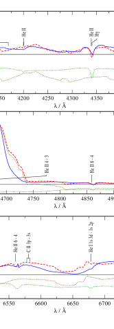
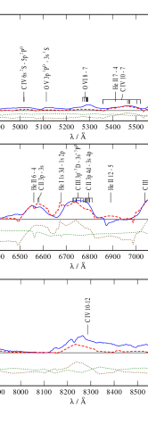
Figure 30: Same as Fig. 29, but shows the normalized FLAMES (panel 1-3) and FORS2 (panel 4-6) spectra.

Appendix C Spectral fits of the OB stars

We present the spectral fits of all the OB stars in the N 206 complex analyzed in this study. The upper panel shows the spectral energy distribution with photometry from UV, optical, and infra-red bands. Lower panels show the normalized VLT-FLAMES spectra depicted by blue solid lines. For a few stars the available UV spectra from HST, FUSE, IUE are also included in the lower panels. The observed spectra are over-plotted with PoWR model spectra (red dashed lines). The main parameters of the best-fit models are compiled in Table 3, continued in Table LABEL:table:App_stellarparameters

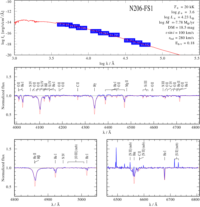
Figure 31: Spectral fit for N206-FS1

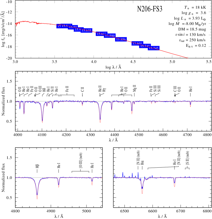
Figure 32: Spectral fit for N206-FS3

Figure 33: Spectral fit for N206-FS5

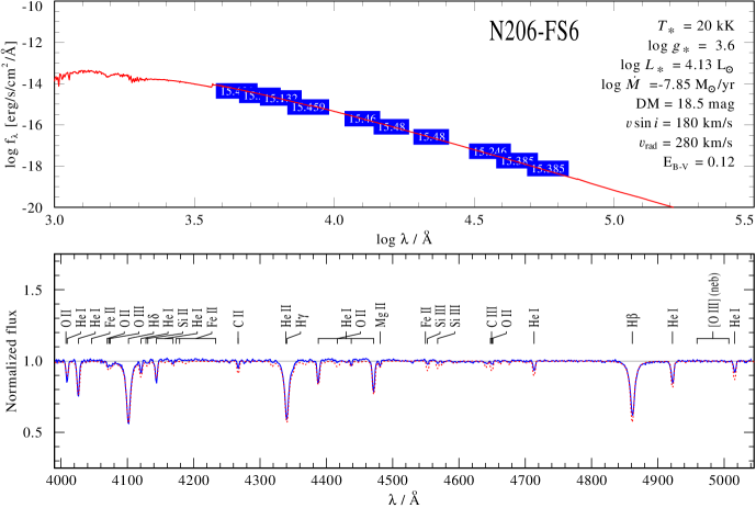
Figure 34: Spectral fit for N206-FS6

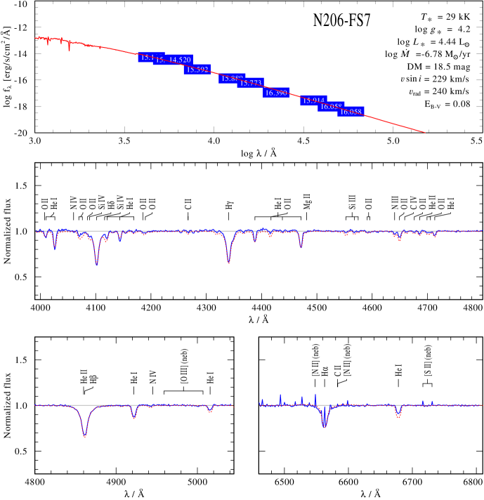
Figure 35: Spectral fit for N206-FS7

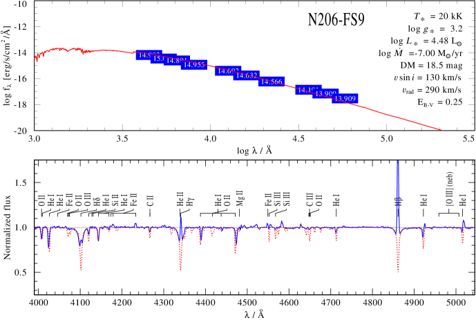
Figure 36: Spectral fit for N206-FS9

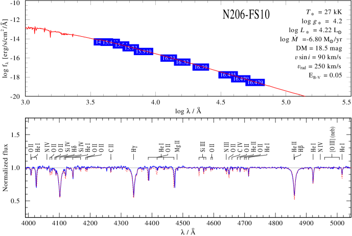
Figure 37: Spectral fit for N206-FS10

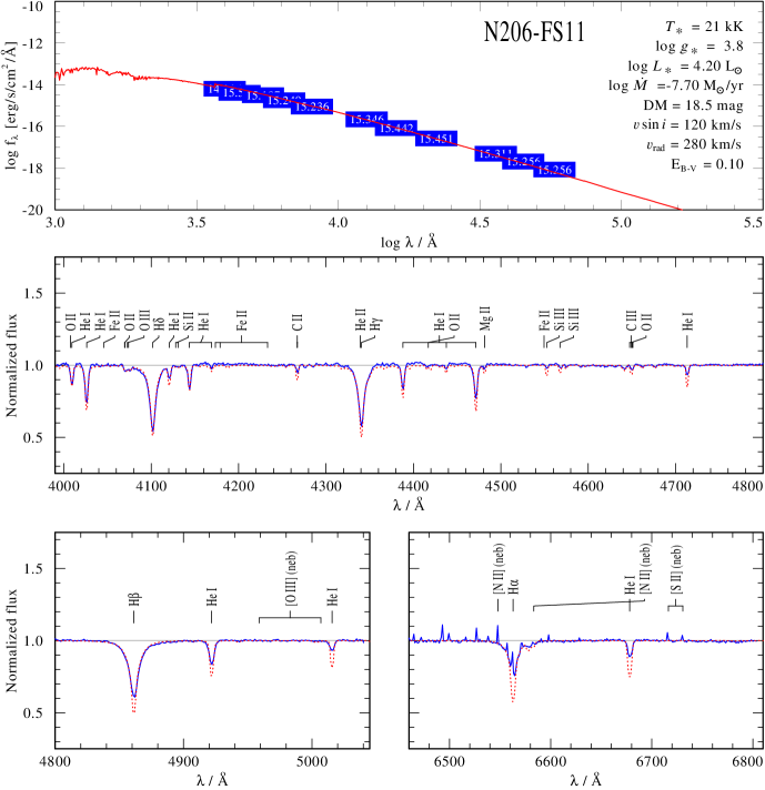
Figure 38: Spectral fit for N206-FS11

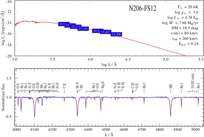
Figure 39: Spectral fit for N206-FS12

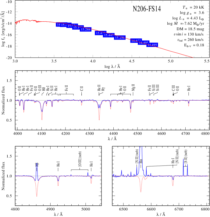
Figure 40: Spectral fit for N206-FS14

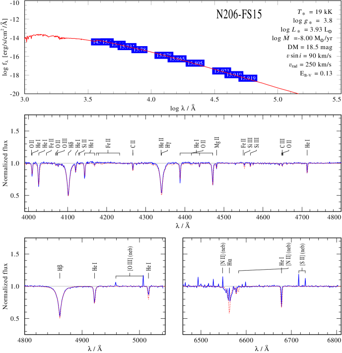
Figure 41: Spectral fit for N206-FS15

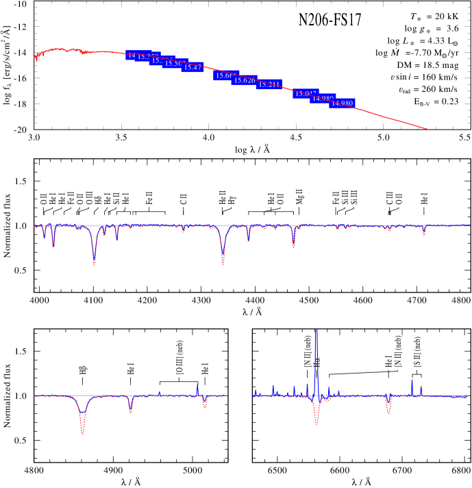
Figure 42: Spectral fit for N206-FS17

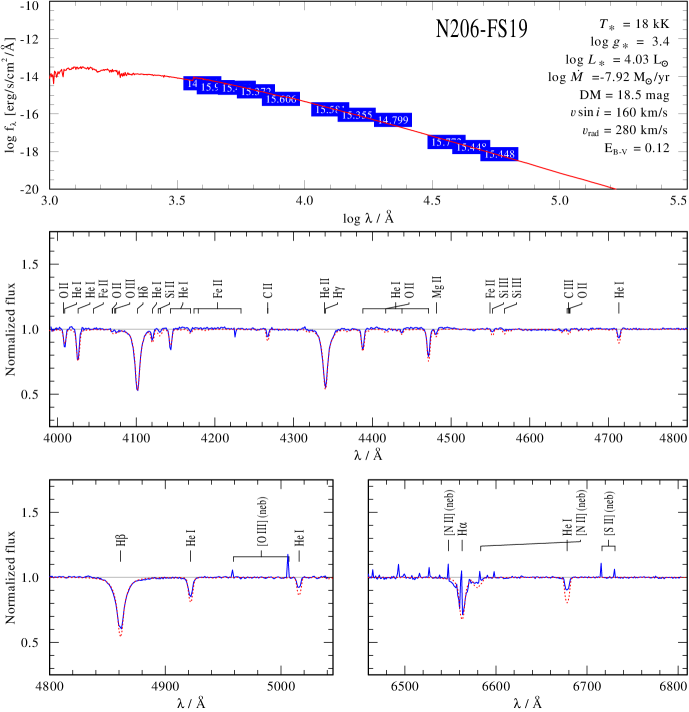
Figure 43: Spectral fit for N206-FS19

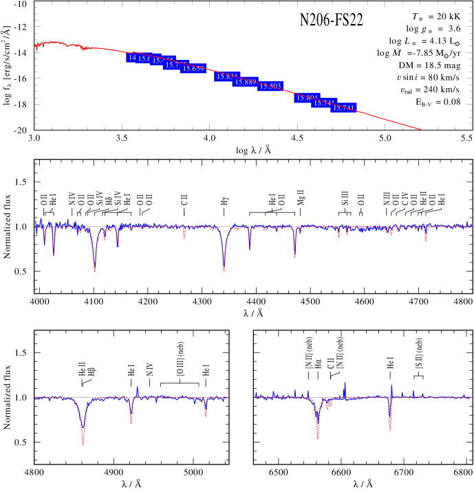
Figure 44: Spectral fit for N206-FS22

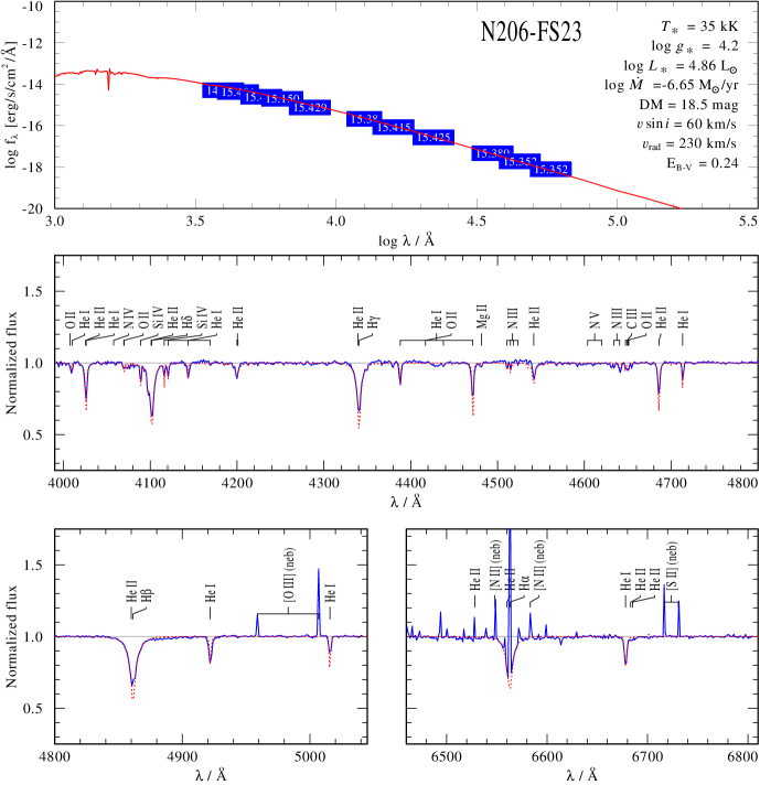
Figure 45: Spectral fit for N206-FS23

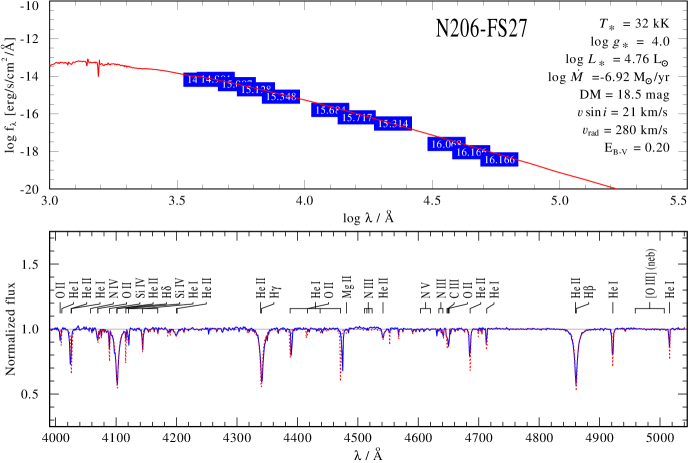
Figure 46: Spectral fit for N206-FS27

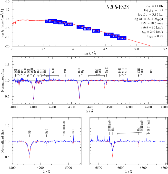
Figure 47: Spectral fit for N206-FS28

Figure 48: Spectral fit for N206-FS29

Figure 49: Spectral fit for N206-FS30

Figure 50: Spectral fit for N206-FS31

Figure 51: Spectral fit for N206-FS32

Figure 52: Spectral fit for N206-FS33

Figure 53: Spectral fit for N206-FS34

Figure 54: Spectral fit for N206-FS36

Figure 55: Spectral fit for N206-FS37

Figure 56: Spectral fit for N206-FS38

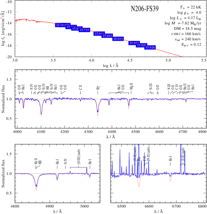
Figure 57: Spectral fit for N206-FS39

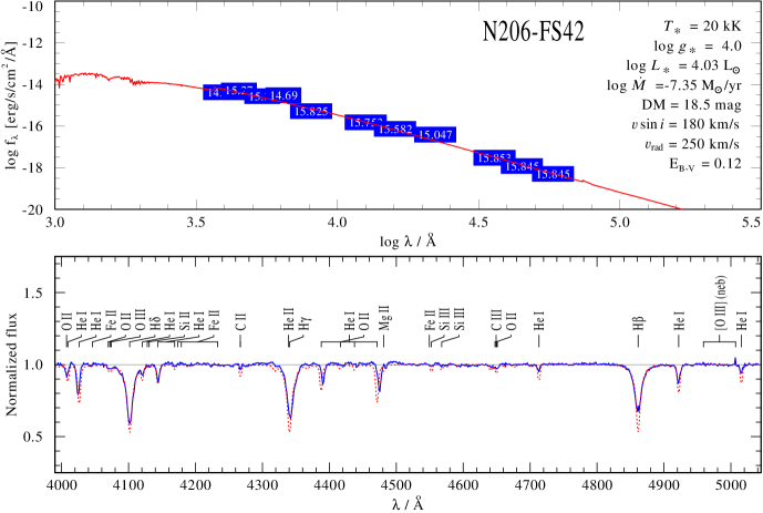
Figure 58: Spectral fit for N206-FS42

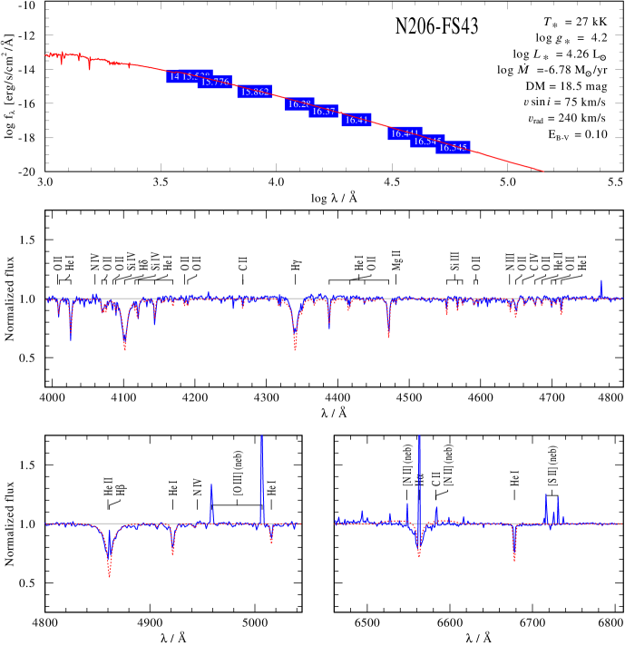
Figure 59: Spectral fit for N206-FS43

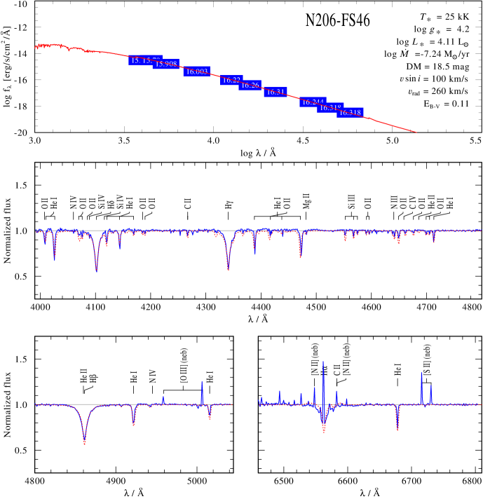
Figure 60: Spectral fit for N206-FS46

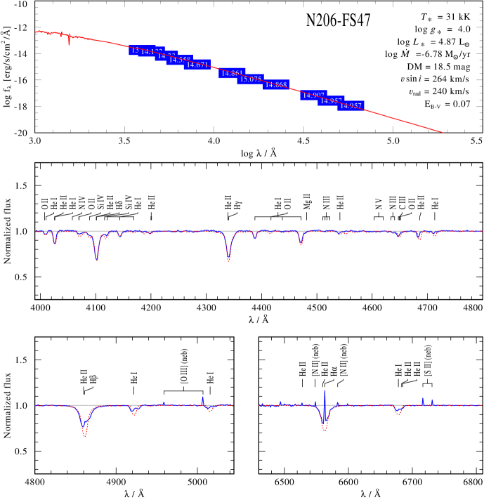
Figure 61: Spectral fit for N206-FS47

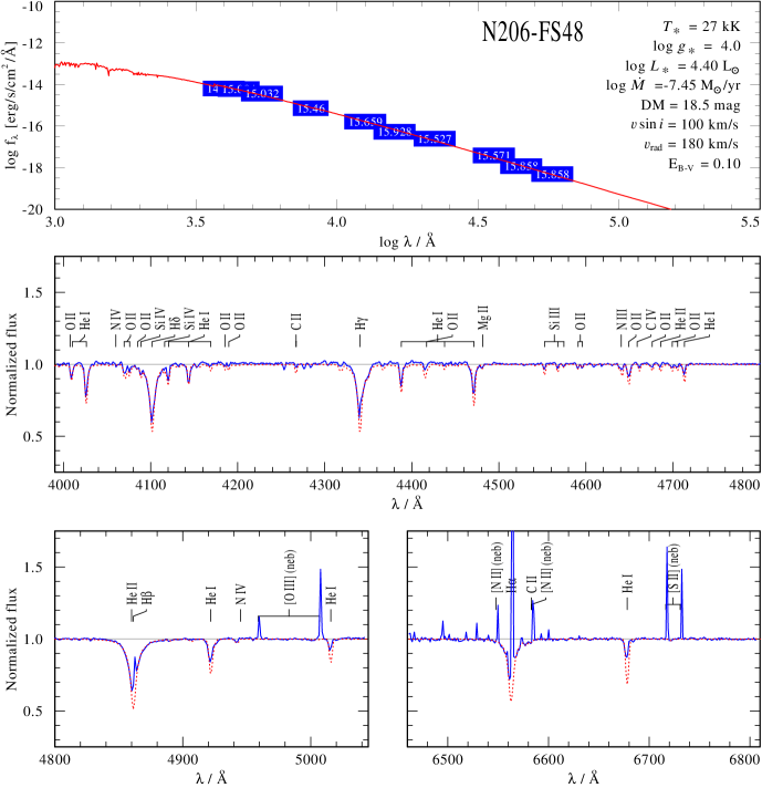
Figure 62: Spectral fit for N206-FS48

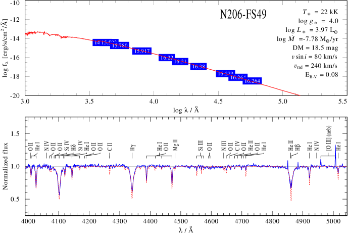
Figure 63: Spectral fit for N206-FS49

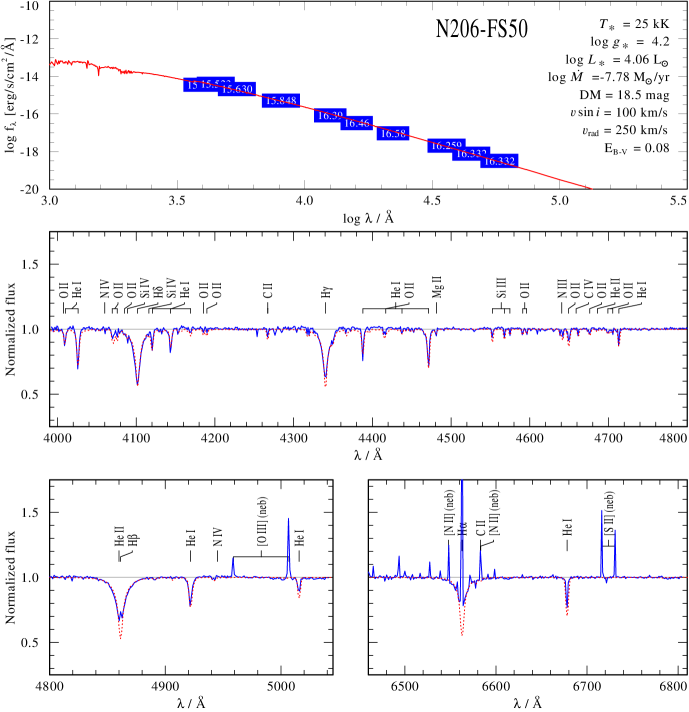
Figure 64: Spectral fit for N206-FS50

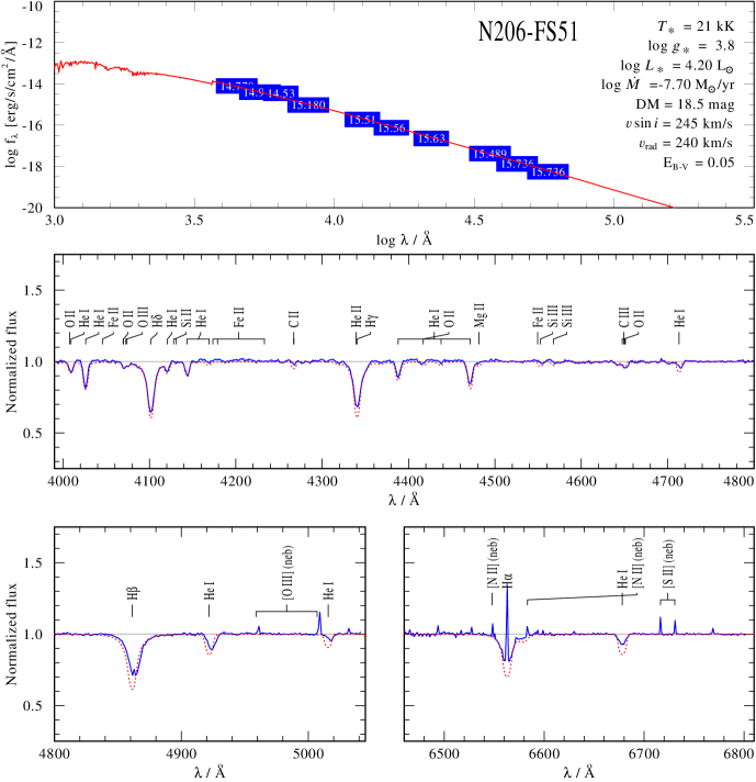
Figure 65: Spectral fit for N206-FS51

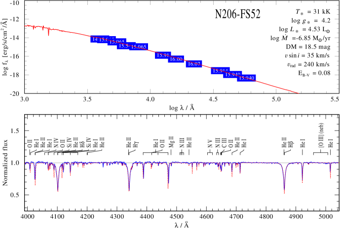
Figure 66: Spectral fit for N206-FS52

Figure 67: Spectral fit for N206-FS55

Figure 68: Spectral fit for N206-FS56

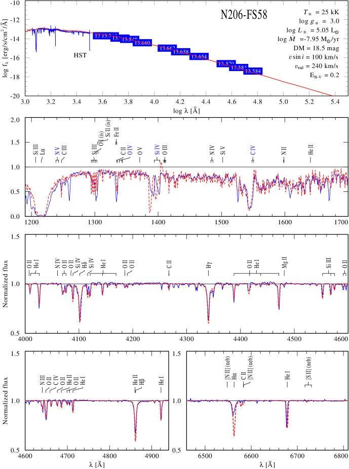
Figure 69: Spectral fit for N206-FS58

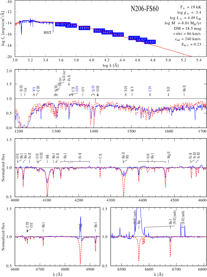
Figure 70: Spectral fit for N206-FS60

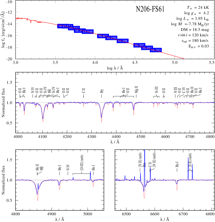
Figure 71: Spectral fit for N206-FS61

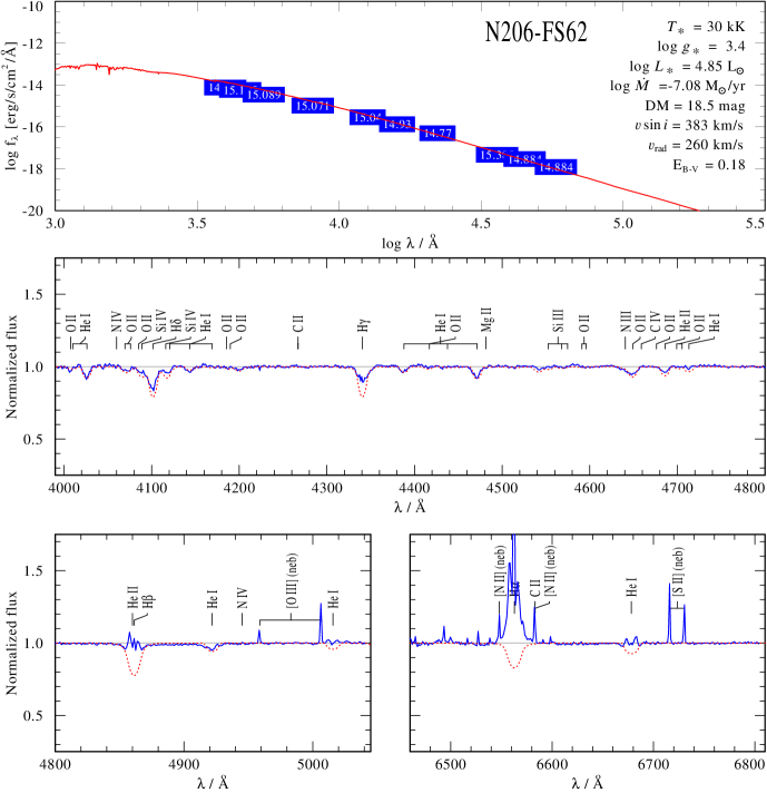
Figure 72: Spectral fit for N206-FS62

Figure 73: Spectral fit for N206-FS64

Figure 74: Spectral fit for N206-FS65

Figure 75: Spectral fit for N206-FS68

Figure 76: Spectral fit for N206-FS69

Figure 77: Spectral fit for N206-FS73

Figure 78: Spectral fit for N206-FS74

Figure 79: Spectral fit for N206-FS75

Figure 80: Spectral fit for N206-FS77

Figure 81: Spectral fit for N206-FS78

Figure 82: Spectral fit for N206-FS80

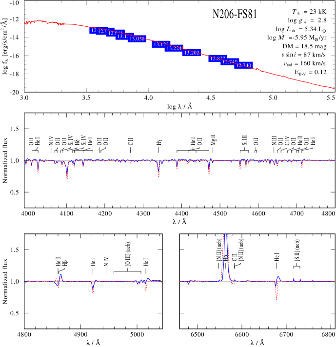
Figure 83: Spectral fit for N206-FS81

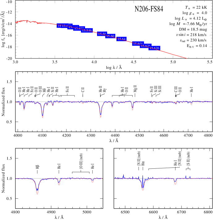
Figure 84: Spectral fit for N206-FS84

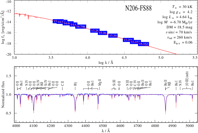
Figure 85: Spectral fit for N206-FS88

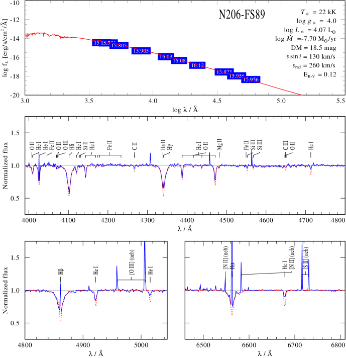
Figure 86: Spectral fit for N206-FS89

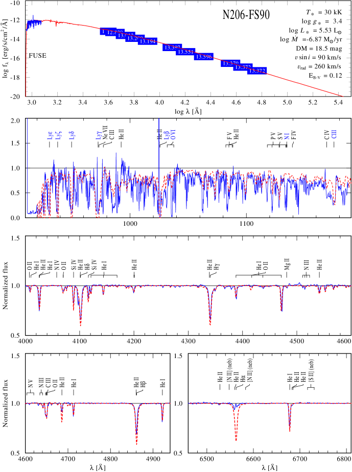
Figure 87: Spectral fit for N206-FS90

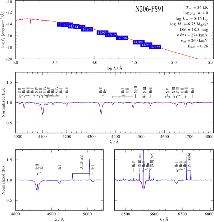
Figure 88: Spectral fit for N206-FS91

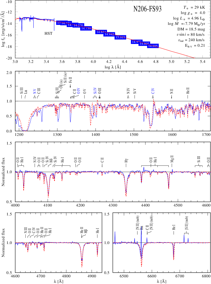
Figure 89: Spectral fit for N206-FS93

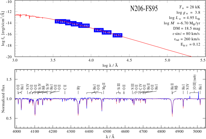
Figure 90: Spectral fit for N206-FS95

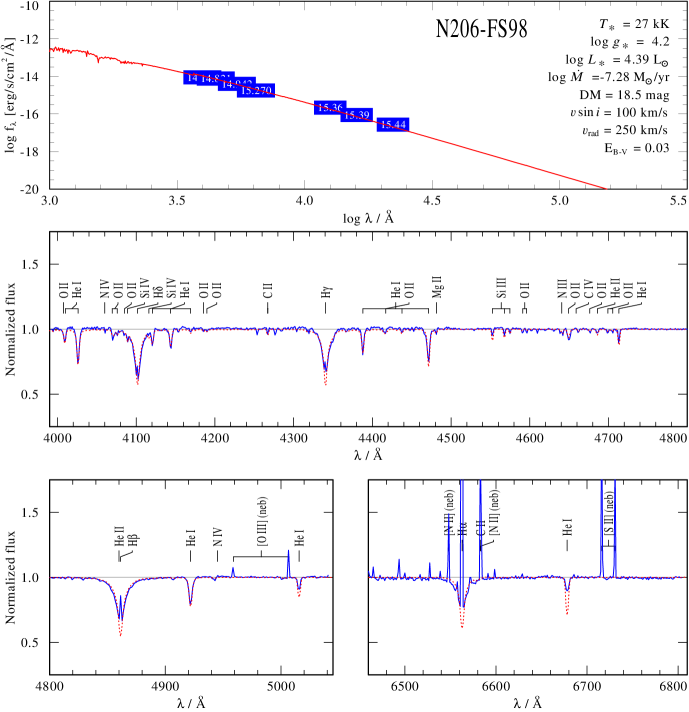
Figure 91: Spectral fit for N206-FS98

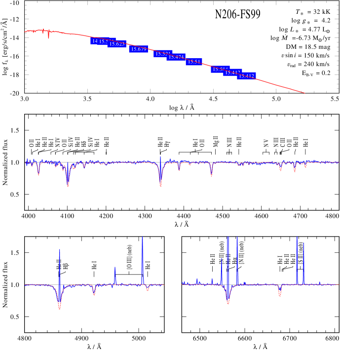
Figure 92: Spectral fit for N206-FS99

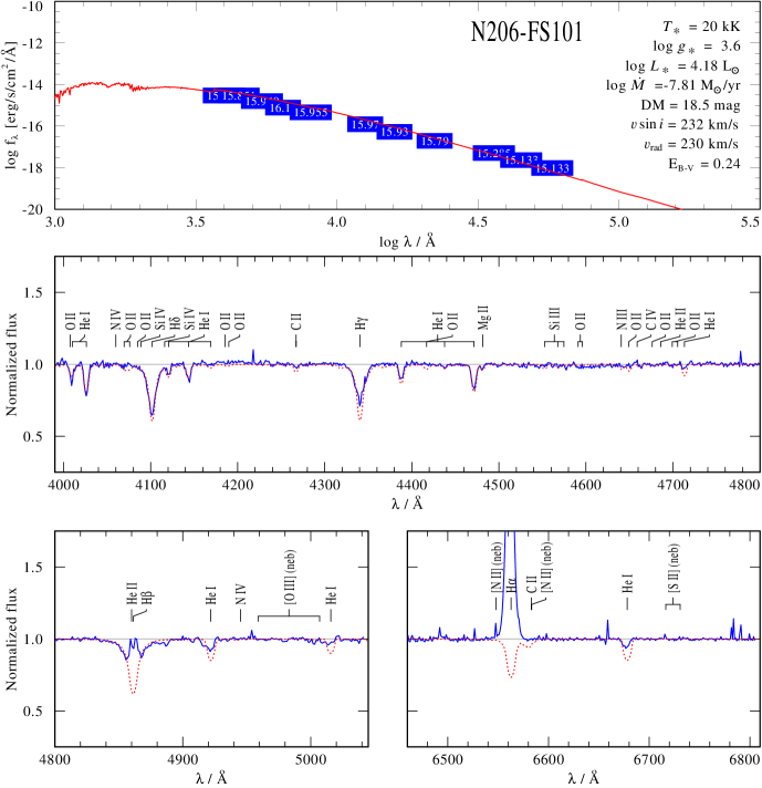
Figure 93: Spectral fit for N206-FS101

Figure 94: Spectral fit for N206-FS103

Figure 95: Spectral fit for N206-FS104

Figure 96: Spectral fit for N206-FS105

Figure 97: Spectral fit for N206-FS107

Figure 98: Spectral fit for N206-FS108

Figure 99: Spectral fit for N206-FS109

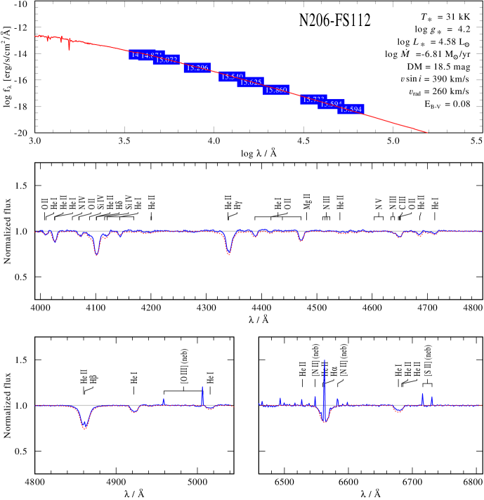
Figure 100: Spectral fit for N206-FS112

Figure 101: Spectral fit for N206-FS113

Figure 102: Spectral fit for N206-FS116

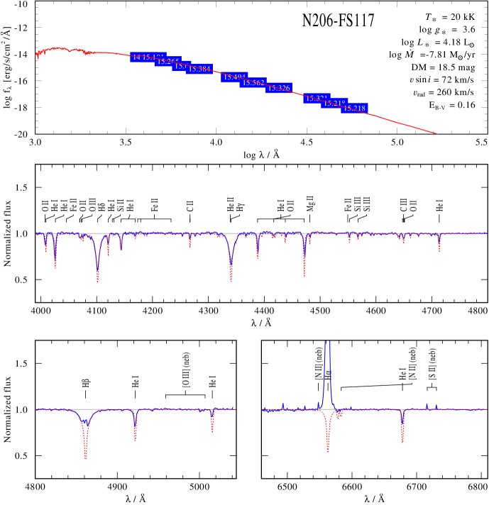
Figure 103: Spectral fit for N206-FS117

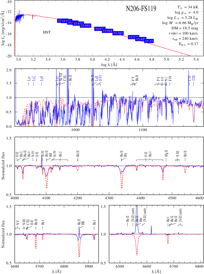
Figure 104: Spectral fit for N206-FS119

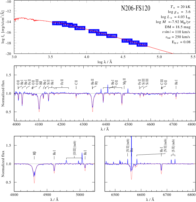
Figure 105: Spectral fit for N206-FS120

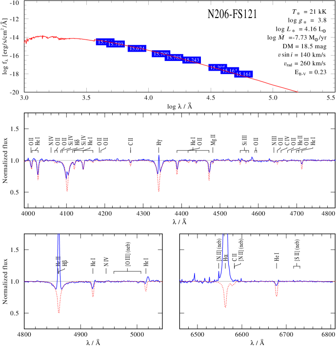
Figure 106: Spectral fit for N206-FS121

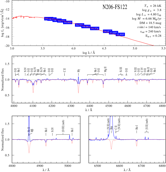
Figure 107: Spectral fit for N206-FS122

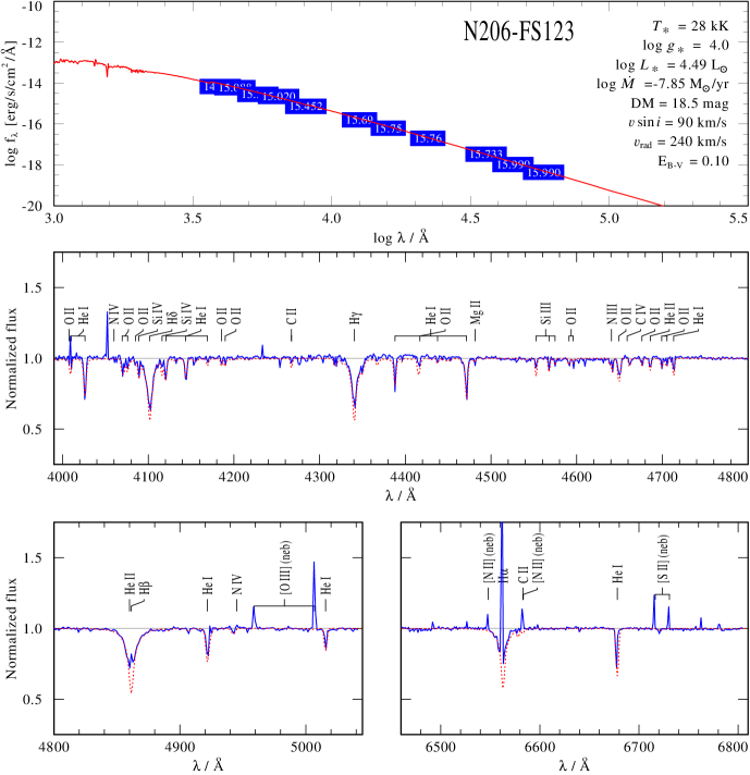
Figure 108: Spectral fit for N206-FS123

Figure 109: Spectral fit for N206-FS125

Figure 110: Spectral fit for N206-FS126

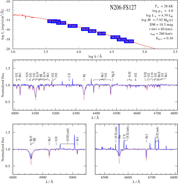
Figure 111: Spectral fit for N206-FS127

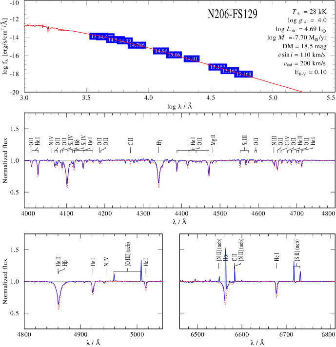
Figure 112: Spectral fit for N206-FS129

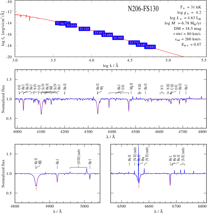
Figure 113: Spectral fit for N206-FS130

Figure 114: Spectral fit for N206-FS132

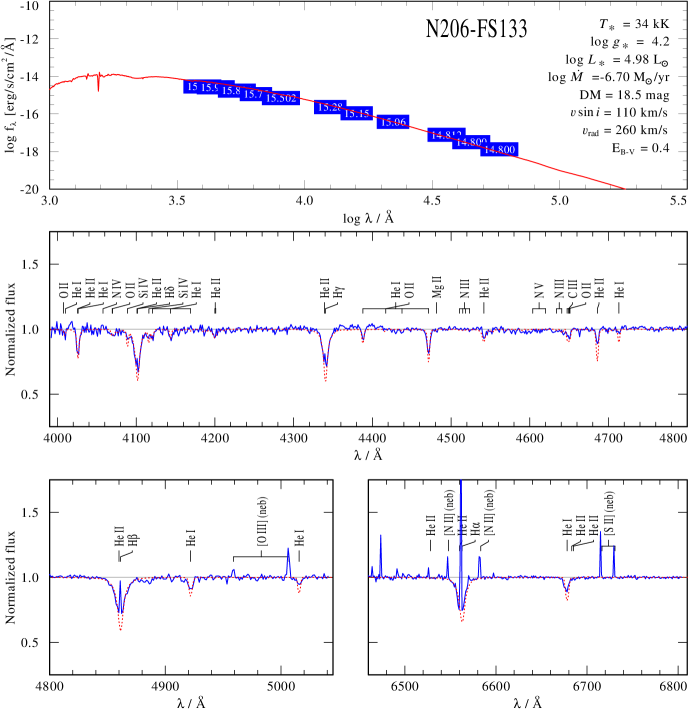
Figure 115: Spectral fit for N206-FS133

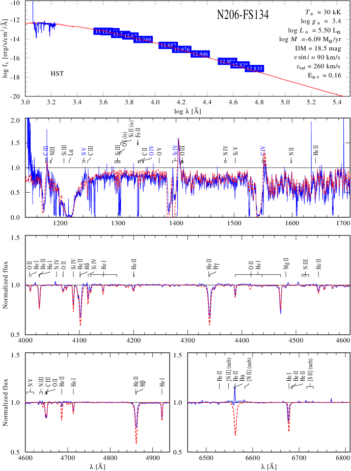
Figure 116: Spectral fit for N206-FS134

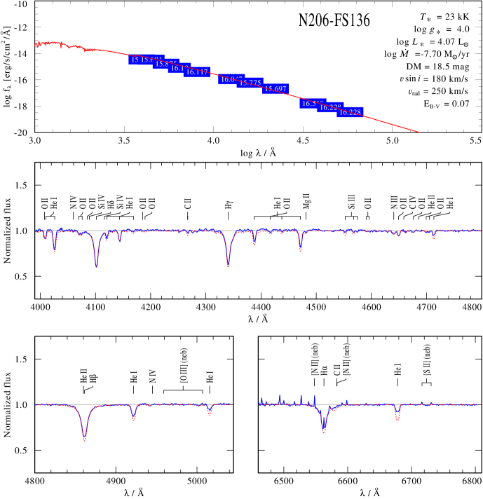
Figure 117: Spectral fit for N206-FS136

Figure 118: Spectral fit for N206-FS138

Figure 119: Spectral fit for N206-FS139

Figure 120: Spectral fit for N206-FS141

Figure 121: Spectral fit for N206-FS142

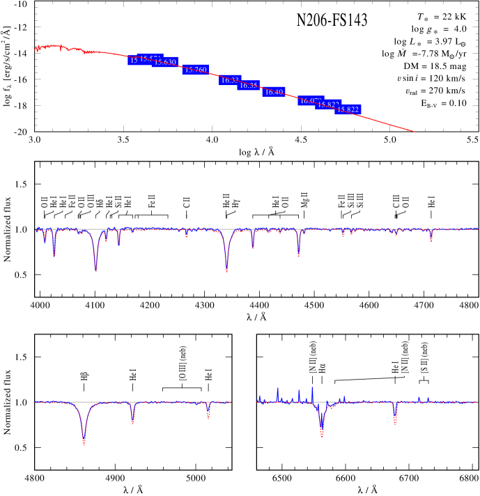
Figure 122: Spectral fit for N206-FS143

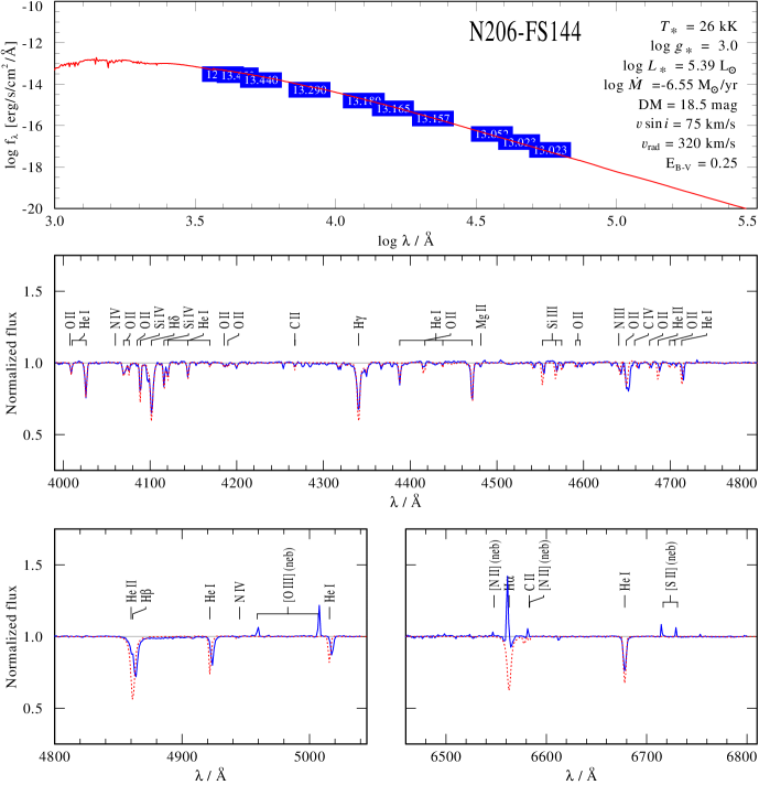
Figure 123: Spectral fit for N206-FS144

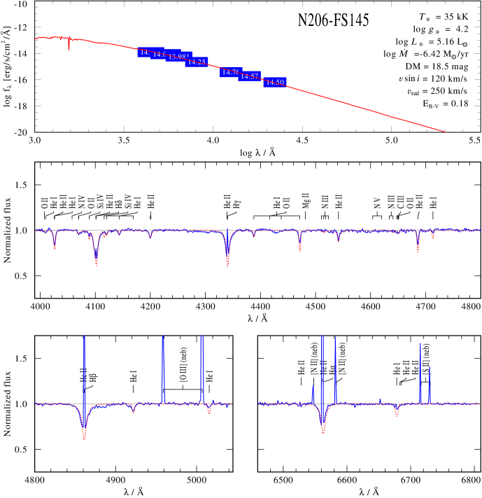
Figure 124: Spectral fit for N206-FS145

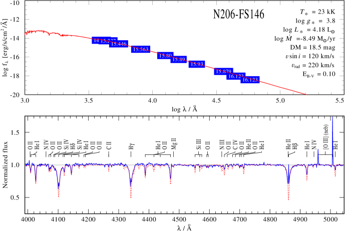
Figure 125: Spectral fit for N206-FS146

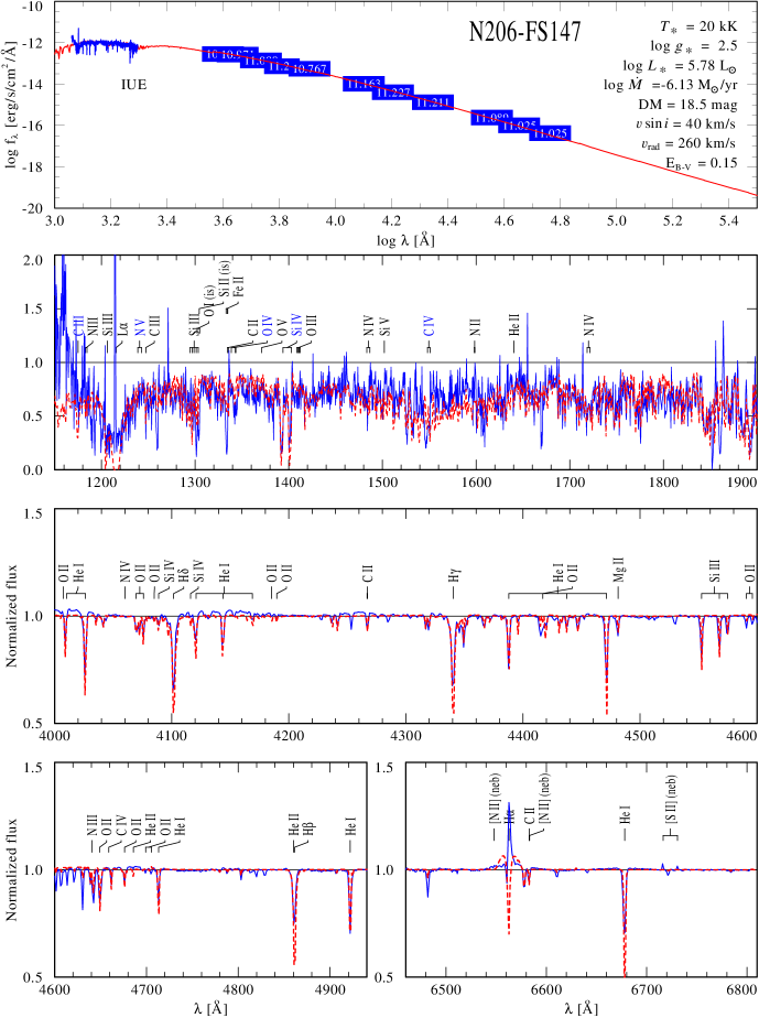
Figure 126: Spectral fit for N206-FS147

Figure 127: Spectral fit for N206-FS148

Figure 128: Spectral fit for N206-FS149

Figure 129: Spectral fit for N206-FS150

Figure 130: Spectral fit for N206-FS151

Figure 131: Spectral fit for N206-FS153

Figure 132: Spectral fit for N206-FS154

Figure 133: Spectral fit for N206-FS155

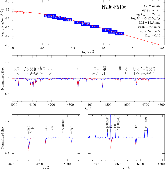
Figure 134: Spectral fit for N206-FS156

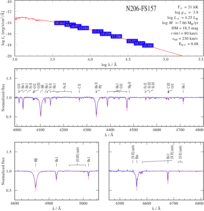
Figure 135: Spectral fit for N206-FS157

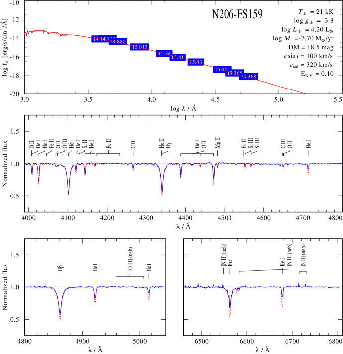
Figure 136: Spectral fit for N206-FS159

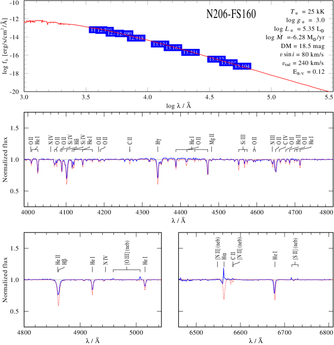
Figure 137: Spectral fit for N206-FS160

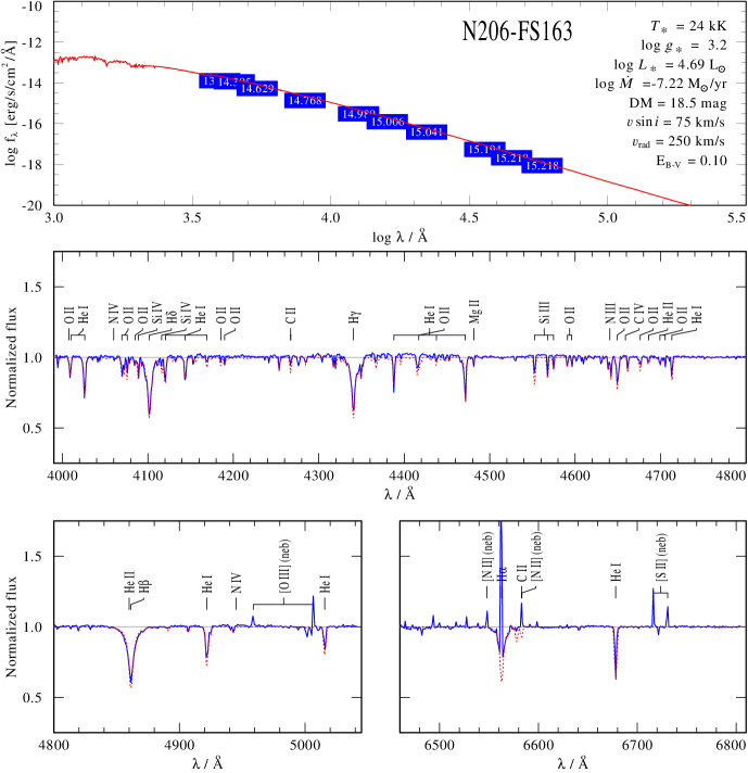
Figure 138: Spectral fit for N206-FS163

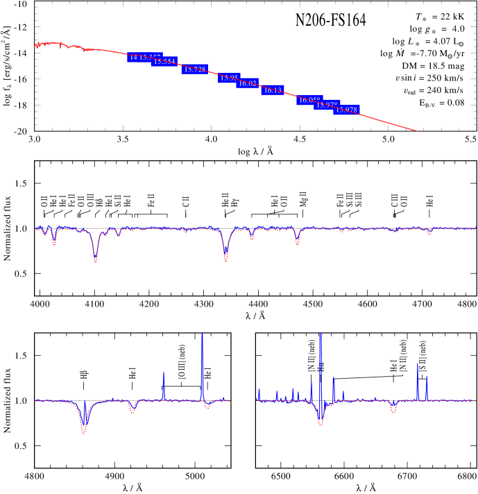
Figure 139: Spectral fit for N206-FS164

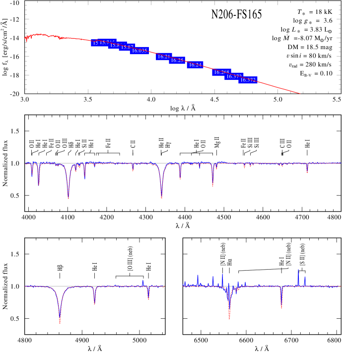
Figure 140: Spectral fit for N206-FS165

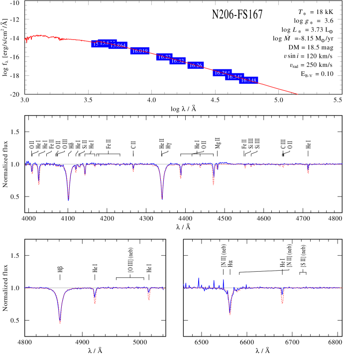
Figure 141: Spectral fit for N206-FS167

Figure 142: Spectral fit for N206-FS168

Figure 143: Spectral fit for N206-FS170

Figure 144: Spectral fit for N206-FS172

Figure 145: Spectral fit for N206-FS173

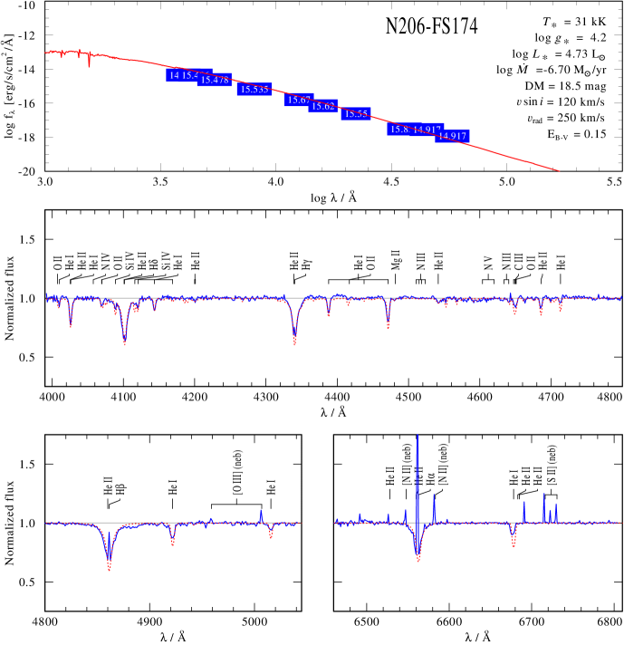
Figure 146: Spectral fit for N206-FS174

Figure 147: Spectral fit for N206-FS175

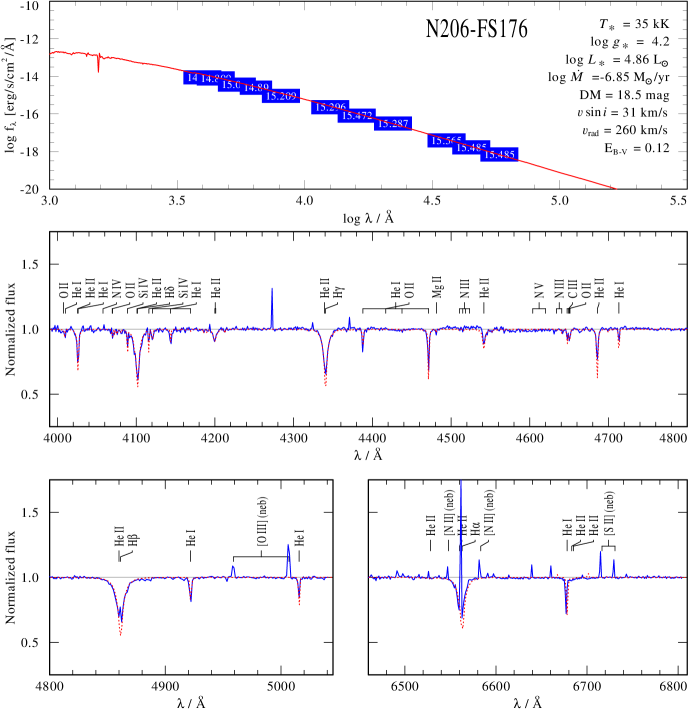
Figure 148: Spectral fit for N206-FS176

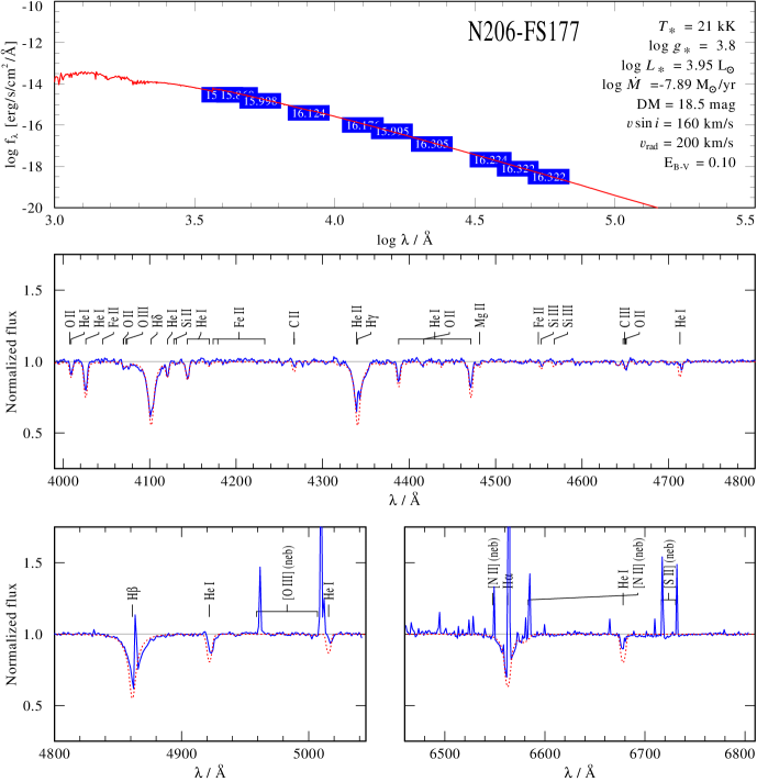
Figure 149: Spectral fit for N206-FS177

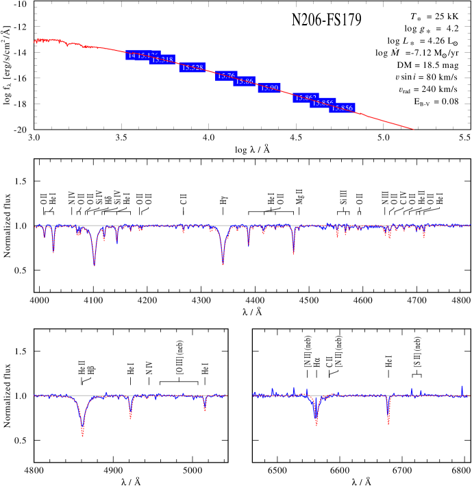
Figure 150: Spectral fit for N206-FS179

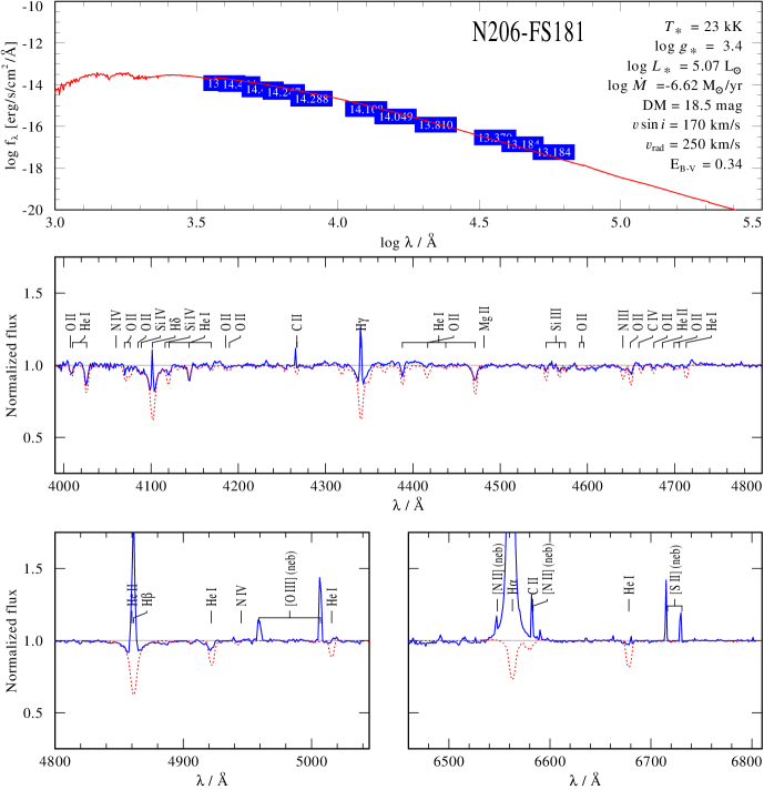
Figure 151: Spectral fit for N206-FS181

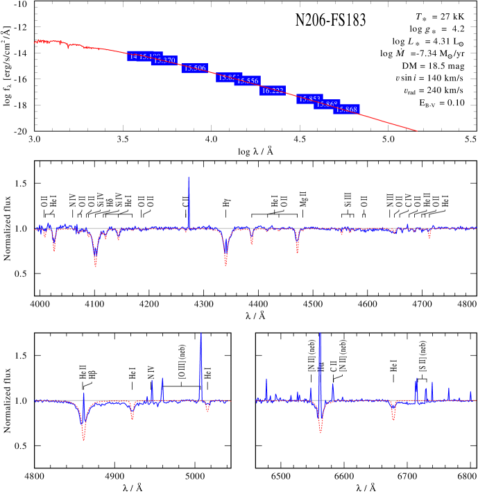
Figure 152: Spectral fit for N206-FS183

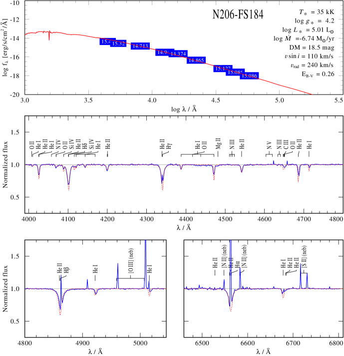
Figure 153: Spectral fit for N206-FS184

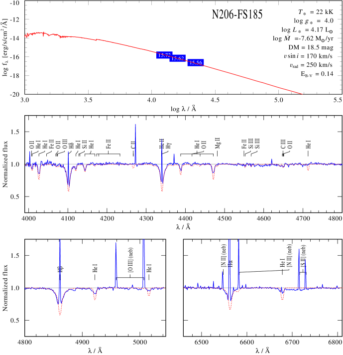
Figure 154: Spectral fit for N206-FS185

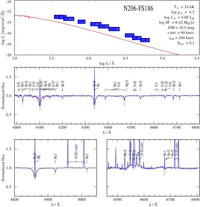
Figure 155: Spectral fit for N206-FS186

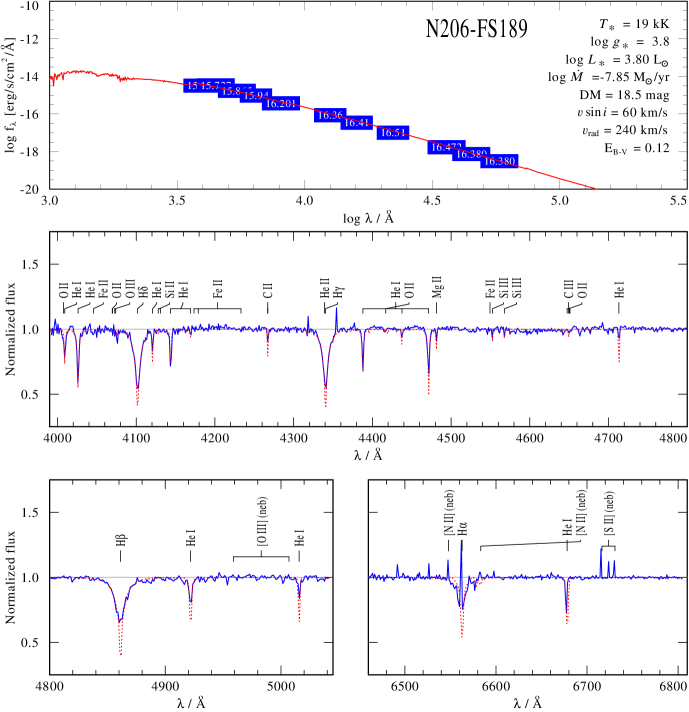
Figure 156: Spectral fit for N206-FS189

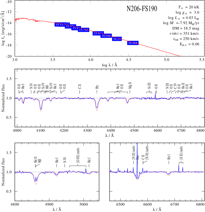
Figure 157: Spectral fit for N206-FS190

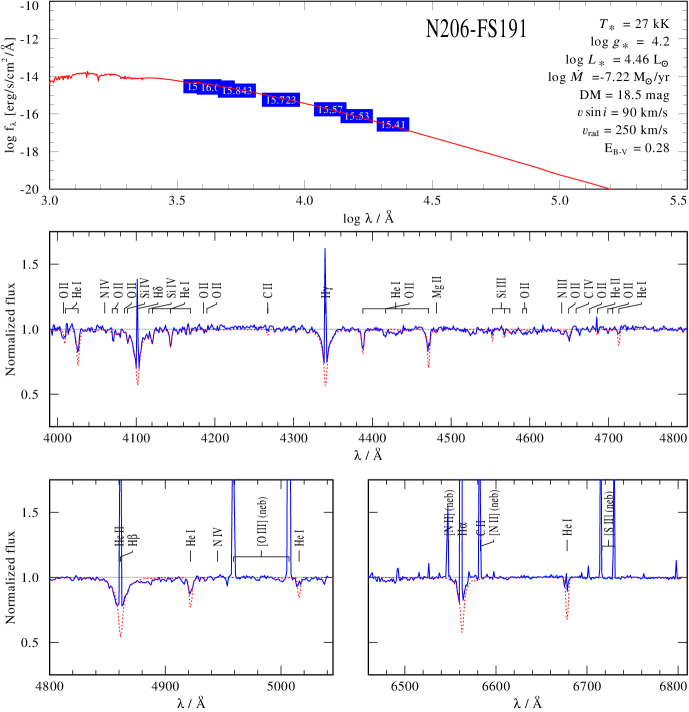
Figure 158: Spectral fit for N206-FS191

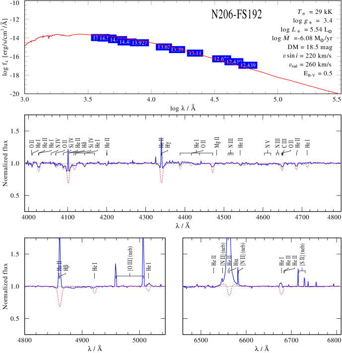
Figure 159: Spectral fit for N206-FS192

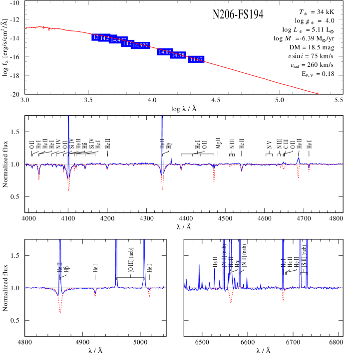
Figure 160: Spectral fit for N206-FS194

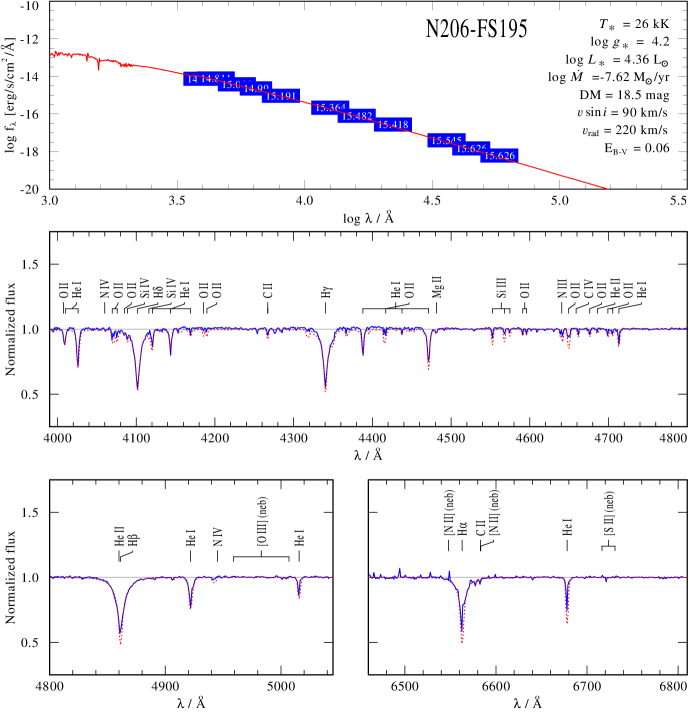
Figure 161: Spectral fit for N206-FS195

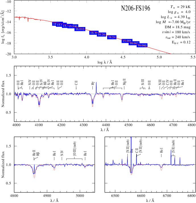
Figure 162: Spectral fit for N206-FS196

Figure 163: Spectral fit for N206-FS197

Figure 164: Spectral fit for N206-FS198

Figure 165: Spectral fit for N206-FS200

Figure 166: Spectral fit for N206-FS201

Figure 167: Spectral fit for N206-FS202

Figure 168: Spectral fit for N206-FS204

Figure 169: Spectral fit for N206-FS205

Figure 170: Spectral fit for N206-FS206

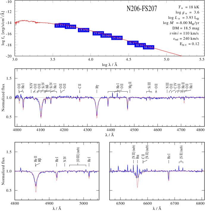
Figure 171: Spectral fit for N206-FS207

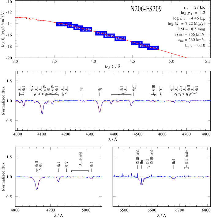
Figure 172: Spectral fit for N206-FS209

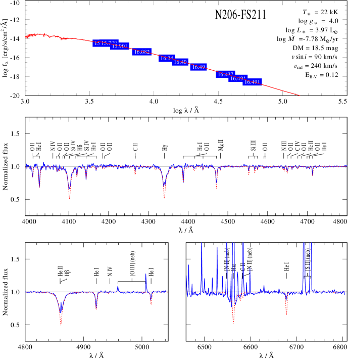
Figure 173: Spectral fit for N206-FS211

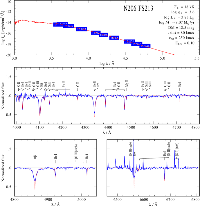
Figure 174: Spectral fit for N206-FS213

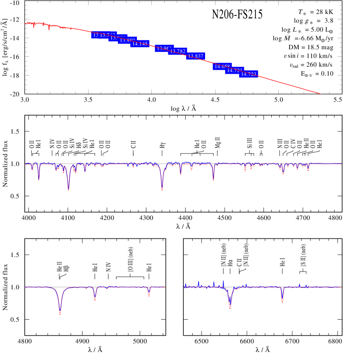
Figure 175: Spectral fit for N206-FS215

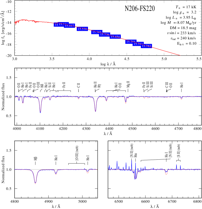
Figure 176: Spectral fit for N206-FS220

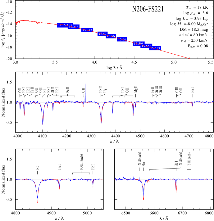
Figure 177: Spectral fit for N206-FS221

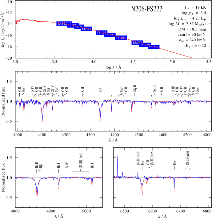
Figure 178: Spectral fit for N206-FS222

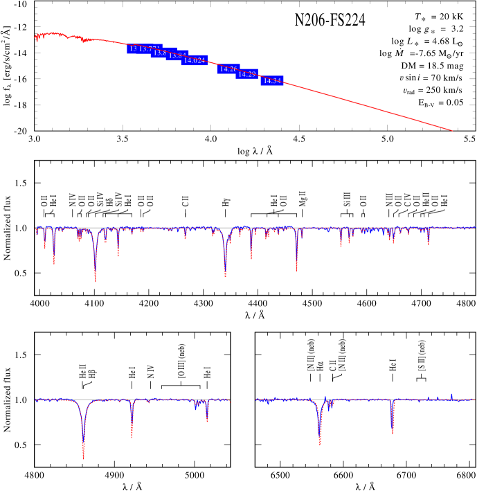
Figure 179: Spectral fit for N206-FS224

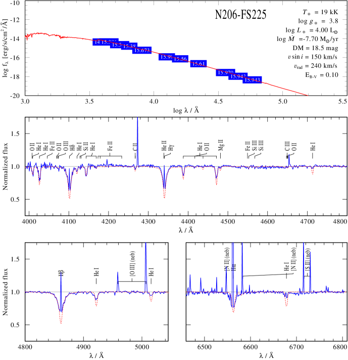
Figure 180: Spectral fit for N206-FS225

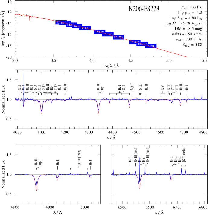
Figure 181: Spectral fit for N206-FS229

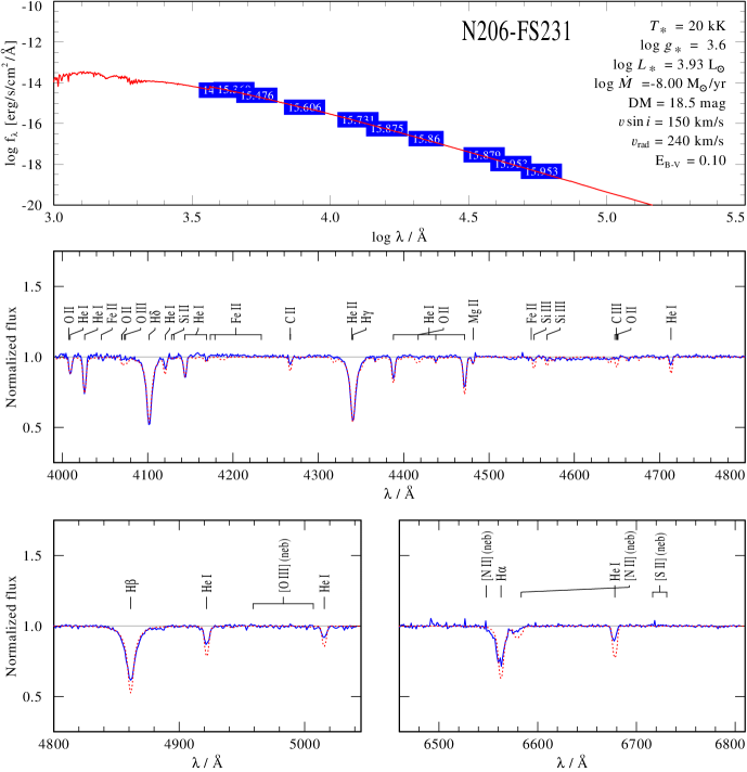
Figure 182: Spectral fit for N206-FS231

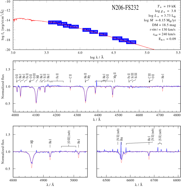
Figure 183: Spectral fit for N206-FS232

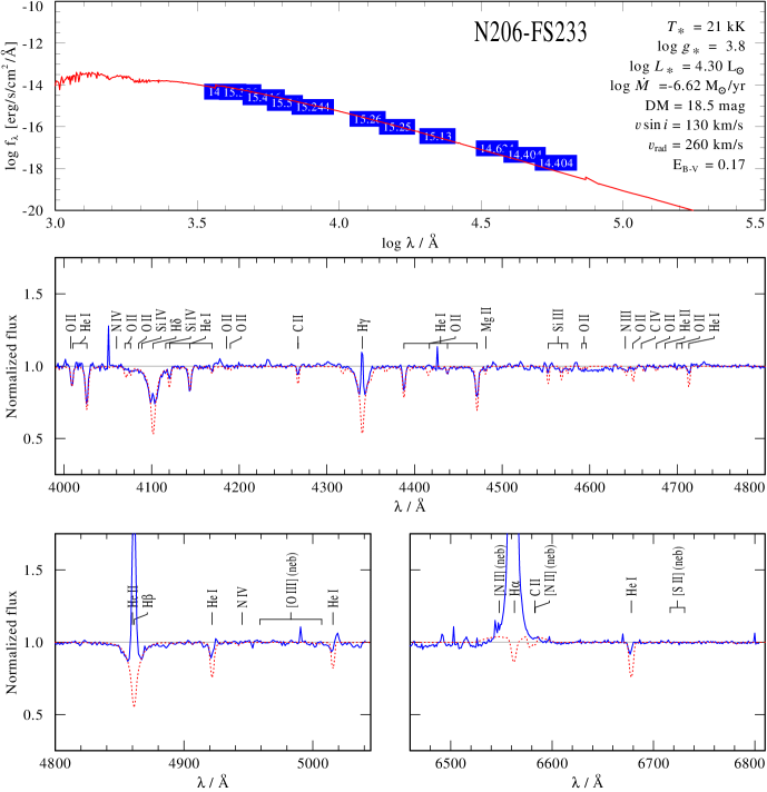
Figure 184: Spectral fit for N206-FS233

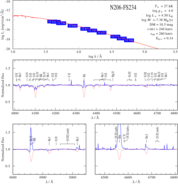
Figure 185: Spectral fit for N206-FS234