Playing with Repetitions in Data Words
Using Energy Games

Abstract.

We introduce two-player games which build words over infinite alphabets, and we study the problem of checking the existence of winning strategies. These games are played by two players, who take turns in choosing valuations for variables ranging over an infinite data domain, thus generating multi-attributed data words. The winner of the game is specified by formulas in the Logic of Repeating Values, which can reason about repetitions of data values in infinite data words. We prove that it is undecidable to check if one of the players has a winning strategy, even in very restrictive settings. However, we prove that if one of the players is restricted to choose valuations ranging over the Boolean domain, the games are effectively equivalent to single-sided games on vector addition systems with states (in which one of the players can change control states but cannot change counter values), known to be decidable and effectively equivalent to energy games.

Previous works have shown that the satisfiability problem for various variants of the logic of repeating values is equivalent to the reachability and coverability problems in vector addition systems. Our results raise this connection to the level of games, augmenting further the associations between logics on data words and counter systems.

1. Introduction

Words over an unbounded domain —known as data words— is a structure that appears in many scenarios, as abstractions of timed words, runs of counter automata, runs of concurrent programs with an unbounded number of processes, traces of reactive systems, and more broadly as abstractions of any record of the run of processes handling unbounded resources. Here, we understand a data word as a (possibly infinite) word in which every position carries a vector of elements from a possibly infinite domain (e.g., a vector of numbers).

Many specification languages have been proposed to specify properties of data words, both in terms of automata [18, 21] and logics [5, 12, 15, 13]. One of the most basic mechanisms for expressing properties on these structures is based on whether a data value at a given position is repeated either locally (e.g., in the $2$^nd component of the vector at the $4$^th future position), or remotely (e.g., in the $1$^st component of a vector at some position in the past). This has led to the study of linear temporal logic extended with these kind of tests, called Logic of Repeating Values (LRV) [10]. The satisfiability problem for LRV is inter-reducible with the reachability problem for Vector Addition Systems with States (VASS), and when the logic is restricted to testing remote repetitions only in the future, it is inter-reducible with the coverability problem for VASS [10, 11]. These connections also extend to data trees and branching VASS [3].

Previous works on data words have been centered around the satisfiability, containment, or model checking problems. Here, we initiate the study of two-player games on such structures, motivated by the realizability problem of reactive systems (hardware, operating systems, communication protocols). A reactive system keeps interacting with the environment in which it is functioning, and a data word can be seen as a trace of this interaction. The values of some variables are decided by the system and some by the environment. The reactive system has to satisfy a specified property, given as a logical formula over data words. The realizability problem asks whether it is possible that there exists a system that always satisfies the specified property, irrespective of what the environment does. This can be formalized as the existence of a winning strategy for a two-player game that is defined to this end. In this game, there are two sets of variables. Valuations for one set of variables are decided by the system player (representing the reactive system) and for the other set of variables, valuations are decided by the environment player (representing the environment in which the reactive system is functioning). The two players take turns giving valuations to their respective variables and build an infinite sequence of valuations. The system player wins a game if the resulting sequence satisfies the specified logical formula. Motivated by the realizability problem of Church [8], the question of existence of winning strategies in such games are studied extensively (starting from [19]) for the case where variables are Boolean and the logic used is propositional linear temporal logic. To the best of our knowledge there have been no works on the more general setup of infinite domains. This work can be seen as a first step towards considering richer structures, this being the case of an infinite set with an equivalence relation.

Contributions

By combining known relations between satisfiability of (fragments of) LRV and (control state) reachability in VASS [10, 11] with existing knowledge about realizability games ([19] and numerous papers expanding on it), it is not difficult to show that realizability games for LRV are related to games on VASS. Using known results about undecidability of games on VASS, it is again not difficult to show that realizability games for LRV are undecidable. Among others, one way to get decidable games on VASS is to make the game asymmetric, letting one player only change control states, while the other player can additionally change values in counters, resulting in the so called single-sided VASS games [1]. Our first contribution in this paper is to identify that the corresponding asymmetry in LRV realizability is to give only Boolean variables to one of the players and let the logic test only for remote repetitions in the past (and disallow testing for remote repetitions in the future). Once this identification of the fragment is made, the proof of its inter-reducibility with single-sided VASS games follows more or less along expected lines by adapting techniques developed in [10, 11].

To obtain the fragment mentioned in the previous paragraph, we impose two restrictions; one is to restrict one of the players to Boolean variables and the other is to dis-allow testing for remote repetitions in the future. Our next contribution in this paper is to prove that lifting either of these restrictions lead to undecidability. A common feature in similar undecidability proofs (e.g., undecidability of VASS games [2]) is a reduction from the reachability problem for $2$-counter machines (details follow in the next section) in which one of the players emulates the moves of the counter machine while the other player catches the first player in case of cheating. Our first undecidability proof uses a new technique where the two players cooperate to emulate the moves of the counter machine and one of the players has the additional task of detecting cheating. Another common feature of similar undecidability proofs is that emulating zero testing transitions of the counter machine is difficult while emulating incrementing and decrementing transitions are easy. Our second undecidability proof uses another new technique in which even emulating decrementing transitions is difficult and requires specific moves by the two players.

Related works

The relations between satisfiability of various logics over data words and the problem of language emptiness for automata models have been explored before. In [5], satisfiability of the two variable fragment of first-order logic on data words is related to reachability in VASS. In [12], satisfiability of LTL extended with freeze quantifiers is related to register automata.

A general framework for games over infinite-state systems with a well-quasi ordering is introduced in [2] and the restriction of downward closure is imposed to get decidability. In [20], the two players follow different rules, making the abilities of the two players asymmetric and leading to decidability. A possibly infinitely branching version of VASS is studied in [6], where decidability is obtained in the restricted case when the goal of the game is to reach a configuration in which one of the counters has the value zero. Games on VASS with inhibitor arcs are studied in [4] and decidability is obtained in the case where one of the players can only increment counters and the other player can not test for zero value in counters. In [7], energy games are studied, which are games on counter systems and the goal of the game is to play for ever without any counter going below zero in addition to satisfying parity conditions on the control states that are visited infinitely often. Energy games are further studied in [1], where they are related to single-sided VASS games, which restrict one of the players to not make any changes to the counters. Closely related perfect half-space games are studied in [9], where it is shown that optimal complexity upper bounds can be obtained for energy games by using perfect half space games.

This paper is an extended version of a preliminary version [14]. Results about nested formulas in sections 7 and 8 are new in this version.

Organization

In Section 2 we define the logic LRV, counter machines, and VASS games. In Section 3 we introduce LRV games. Section 4 shows undecidability results for the fragment of LRV with data repetition tests restricted to past. Section 5 shows the decidability result of past-looking single-sided LRV games. Section 6 shows undecidability of future-looking single-sided LRV games, showing that in some sense the decidability result is maximal. In Section 7, we show that decidability is preserved for past looking single-sided games if we allow nested formulas that can only use past LTL modalities. We show in Section 8 that even past looking single-sided games are undecidable if we allow nested formulas to use future LTL modalities. We conclude in Section 9.

2. Preliminaries

We denote by $\mathbb{Z}$ the set of integers and by $\mathbb{N}$ the set of non-negative integers. We let $\mathbb{N}_{+}$ denote the set of integers that are strictly greater than $0$. For any set $S$, we denote by $S^{*}$ (resp. $S^{\omega}$) the set of all finite (resp. countably infinite) sequences of elements in $S$. For a sequence $\sigma\in S^{*}$, we denote its length by $|\sigma|$. We denote by $\mathcal{P}(S)$ (resp. $\mathcal{P}^{+}(S)$) the set of all subsets (resp. non-empty subsets) of $S$.

Logic of repeating values

We recall the syntax and semantics of the logic of repeating values from [10, 11]. This logic extends the usual propositional linear temporal logic with the ability to reason about repetitions of data values from an infinite domain. We let this logic use both Boolean variables (i.e., propositions) and data variables ranging over an infinite data domain $\mathbb{D}$. The Boolean variables can be simulated by data variables. However, we need to consider fragments of the logic, for which explicitly having Boolean variables is convenient. Let $\textit{BVARS}=\{q,t,\ldots\}$ be a countably infinite set of Boolean variables ranging over $\{\top,\bot\}$, and let $\textit{DVARS}=\{x,y,\ldots\}$ be a countably infinite set of ‘data’ variables ranging over $\mathbb{D}$. We denote by LRV the logic whose formulas are defined as follows:

$$\varphi::= ~{}q~{}|~{}x\approx{\sf X}^{j}y~{}|~{}x\approx\langle\varphi?\rangle y~{}|~{}x\not\approx\langle\varphi?\rangle y~{}|~{}x\approx\langle\varphi?\rangle^{-1}y$$

$$~{}|~{}x\not\approx\langle\varphi?\rangle^{-1}y~{}|~{}\varphi\land\psi~{}|~{}\lnot\varphi~{}|~{}{\sf X}\varphi~{}|~{}\varphi{\sf U}\psi~{}|~{}{\sf X}^{-1}\varphi$$

$$~{}|~{}\varphi{\sf S}\psi~{},~{}\text{where }q\in\textit{BVARS},~{}x,y\in\textit{DVARS},~{}j\in\mathbb{Z}$$

A valuation is the union of a mapping from BVARS to $\{\top,\bot\}$ and a mapping from DVARS to $\mathbb{D}$. A model is a finite or infinite sequence of valuations. We use $\sigma$ to denote models and $\sigma(i)$ denotes the $i$^th valuation in $\sigma$, where $i\in\mathbb{N}_{+}$. For any model $\sigma$ and position $i\in\mathbb{N}_{+}$, the satisfaction relation $\models$ is defined inductively as shown in Table 1. The semantics of temporal operators next (${\sf X}$), previous (${\sf X}^{-1}$), until (${\sf U}$), since (${\sf S}$) and the Boolean connectives are defined in the usual way, but for the sake of completeness we provide their formal definitions. In Table 1, $q\in\textit{BVARS}$, $x,y\in\textit{DVARS}$.

$$\sigma,i\models q \text{ iff }\sigma(i)(q)=\top$$

$$\sigma,i\models x\approx{\sf X}^{j}y \text{ iff }1\leq i+j\leq|\sigma|,~{}\sigma(i)(x)=\sigma(i+j)(y)$$

$$\sigma,i\models x\approx\langle\varphi?\rangle y \text{ iff }\exists j>i\text{ s.t. }\sigma(i)(x)=\sigma(j)(y),~{}\sigma,j\models\varphi$$

$$\sigma,i\models x\not\approx\langle\varphi?\rangle y \text{ iff }\exists j>i\text{ s.t. }\sigma(i)(x)\neq\sigma(j)(y),~{}\sigma,j\models\varphi$$

$$\sigma,i\models x\approx\langle\varphi?\rangle^{-1}y \text{ iff }\exists j<i\text{ s.t. }\sigma(i)(x)=\sigma(j)(y),~{}\sigma,j\models\varphi$$

$$\sigma,i\models x\not\approx\langle\varphi?\rangle^{-1}y \text{ iff }\exists j<i\text{ s.t. }\sigma(i)(x)\neq\sigma(j)(y),~{}\sigma,j\models\varphi$$

$$\sigma,i\models{\sf X}\varphi \text{ iff }\sigma,{i+1}\models\varphi$$

$$\sigma,i\models\varphi{\sf U}\psi \text{ iff }\exists j\geq i\text{ s.t. }\sigma,j\models\psi\text{ and }~{}\forall i\leq k<j,\ \sigma,k\models\varphi$$

$$\sigma,i\models{\sf X}^{-1}\varphi \text{ iff }i>0\text{ and }~{}\sigma,{i-1}\models\varphi$$

$$\sigma,i\models\varphi{\sf S}\psi \text{ iff }\exists j\leq i\text{ s.t. }\sigma,j\models\psi\text{ and }~{}\forall j<k\leq i,\ \sigma,k\models\varphi$$

$$\sigma,i\models\varphi\land\psi \text{ iff }\sigma,i\models\varphi\text{ and }~{}\sigma,i\models\psi$$

$$\sigma,i\models\lnot\varphi \text{ iff }\sigma,i\not\models\varphi$$

Table 1. Semantics of LRV.

Intuitively, the formula $x\approx{\sf X}^{j}y$ tests that the data value mapped to the variable $x$ at the current position repeats in the variable $y$ after $j$ positions. We use the notation ${\sf X}^{i}x\approx{\sf X}^{j}y$ as an abbreviation for the formula ${\sf X}^{i}(x\approx{\sf X}^{j-i}y)$ (assuming without any loss of generality that $i\leq j$). The formula $x\approx\langle\varphi?\rangle y$ tests that the data value mapped to $x$ now repeats in $y$ at a future position that satisfies the nested formula $\varphi$. The formula $x\not\approx\langle\varphi?\rangle y$ is similar but tests for disequality of data values instead of equality. If a model is being built sequentially step by step and these formulas are to be satisfied at a position, they create obligations (for repeating some data values) to be satisfied in some future step. The formulas $x\approx\langle\varphi?\rangle^{-1}y$ and $x\not\approx\langle\varphi?\rangle^{-1}y$ are similar but test for repetitions of data values in past positions.

We consider fragments of LRV in which only past LTL modalities are allowed. Formally, the grammar is:

$$\varphi::=q~{}|~{}x\approx{\sf X}^{-j}y~{}|~{}x\approx\langle\varphi?\rangle^{-1}y~{}|~{}x\not\approx\langle\varphi?\rangle^{-1}y~{}|~{}\varphi\land\psi~{}|~{}\lnot\varphi~{}|~{}{\sf X}^{-1}\varphi~{}|~{}\varphi{\sf S}\psi~{},~{}$$

$$\text{where }q\in\textit{BVARS},~{}x,y\in\textit{DVARS},~{}j\in\mathbb{N}$$ (1)

We append symbols to LRV for denoting syntactic restrictions as shown in the following table. For example, LRV$[\top,\approx,\leftarrow]$ denotes the fragment of LRV in which nested formulas, disequality constraints and future obligations are not allowed. For clarity, we replace $\langle\top?\rangle$ with $\Diamond$ in formulas. E.g., we write $x\approx\langle\top?\rangle y$ as simply $x\approx\Diamond y$.

Symbol	Meaning
$\top$	$\varphi$ has to be $\top$ in $x\approx\langle\varphi?\rangle y$ (no nested formulas)
$\approx$	disequality constraints ($x\not\approx\langle\varphi?\rangle y$ or $x\not\approx\langle\varphi?\rangle^{-1}y$) are not allowed
$\rightarrow$	past obligations ($x\approx\langle\varphi?\rangle^{-1}y$ or $x\not\approx\langle\varphi?\rangle^{-1}y$) are not allowed
$\leftarrow$	future obligations ($x\approx\langle\varphi?\rangle y$ or $x\not\approx\langle\varphi?\rangle y$) are not allowed
$\langle{\sf X}^{-1},{\sf S}\rangle$	${\sf X},{\sf U}$ (and operators derived from them) not allowed in nested formulas (grammar in (1))
$\langle{\sf F}\rangle$	${\sf F}$ operator allowed in nested formulas

Parity games on integer vectors

We recall the definition of games on Vector Addition Systems with States (VASS) from [1]. The game is played between two players: system and environment. A VASS game is a tuple $(Q,C,T,\pi)$ where $Q$ is a finite set of states, $C$ is a finite set of counters, $T$ is a finite set of transitions and $\pi:Q\to\{1,\ldots,p\}$, for some integer $p$, is a colouring function that assigns a number to each state. The set $Q$ is partitioned into two parts $Q^{e}$ (states of environment) and $Q^{s}$ (states of system). A transition in $T$ is a tuple $(q,\mathit{op},q^{\prime})$ where $q,q^{\prime}\in Q$ are the origin and target states and $\mathit{op}$ is an operation of the form $x++$, $x--$ or $\mathit{nop}$, where $x\in C$ is a counter. We say that a transition of a VASS game belongs to environment if its origin belongs to environment; similarly for system. A VASS game is single-sided if every environment transition is of the form $(q,\mathit{nop},q^{\prime})$. It is assumed that every state has at least one outgoing transition.

A configuration of the VASS game is an element $(q,\vec{n})$ of $Q\times\mathbb{N}^{C}$, consisting of a state $q$ and a valuation $\vec{n}$ for the counters. A play of the VASS game begins at a designated initial configuration. The player owning the state of the current configuration (say $(q,\vec{n})$) chooses an outgoing transition (say $(q,\mathit{op},q^{\prime})$) and changes the configuration to $(q^{\prime},\vec{n^{\prime}})$, where $\vec{n^{\prime}}$ is obtained from $\vec{n}$ by incrementing (resp. decrementing) the counter $x$ once, if $\mathit{op}$ is $x++$ (resp. $x--$). If $\mathit{op}=\mathit{nop}$, then $\vec{n^{\prime}}=\vec{n}$. We denote this update as $(q,\vec{n})\xrightarrow{(q,\mathit{op},q^{\prime})}(q^{\prime},\vec{n^{\prime}})$. The play is then continued similarly by the owner of the state of the next configuration. If any player wants to take a transition that decrements some counter, that counter should have a non-zero value before the transition. Note that in a single-sided VASS game, environment cannot change the value of the counters. The game continues forever and results in an infinite sequence of configurations $(q_{0},\vec{n_{0}})(q_{1},\vec{n_{1}})\cdots$. System wins the game if the maximum colour occurring infinitely often in $\pi(q_{0})\pi(q_{1})\pi(q_{2})\cdots$ is even. We assume without loss of generality that from any configuration, at least one transition is enabled (if this condition is not met, we can add extra states and transitions to create an infinite loop ensuring that the owner of the deadlocked configuration loses). In our constructions, we use a generalized form of transitions $q\xrightarrow{\vec{u}}q^{\prime}$ where $\vec{u}\in\mathbb{Z}^{C}$, to indicate that each counter $c$ should be updated by adding $\vec{u}(c)$. Such VASS games can be effectively translated into ones of the form defined in the previous paragraph, preserving winning regions.

A strategy $\mathit{se}$ for environment in a VASS game is a mapping $\mathit{se}:{(Q\times\mathbb{N}^{C})}^{*}\cdot(Q^{e}\times\mathbb{N}^{C})\to T$ such that for all $\gamma\in{(Q\times\mathbb{N}^{C})}^{*}$, all $q^{e}\in Q^{e}$ and all $\vec{n}\in\mathbb{N}^{C}$, $\mathit{se}(\gamma\cdot(q^{e},\vec{n}))$ is a transition whose source state is $q^{e}$. A strategy $\mathit{ss}$ for system is a mapping $\mathit{ss}:{(Q\times\mathbb{N}^{C})}^{*}\cdot(Q^{s}\times\mathbb{N}^{C})\to T$ satisfying similar conditions. Environment plays a game according to a strategy $\mathit{se}$ if the resulting sequence of configurations $(q_{0},\vec{n_{0}})(q_{1},\vec{n_{1}})\cdots$ is such that for all $i\in\mathbb{N}$, $q_{i}\in Q^{e}$ implies $(q_{i},\vec{n}_{i})\xrightarrow{\mathit{se}((q_{0},\vec{n}_{0})(q_{1},\vec{n}_{1})\cdots(q_{i},\vec{n}_{i}))}(q_{i+1},\vec{n}_{i+1})$. The notion is extended to system player similarly. A strategy $\mathit{ss}$ for system is winning if system wins all the games that she plays according to $\mathit{ss}$, irrespective of the strategy used by environment. It was shown in [1] that it is decidable to check whether system has a winning strategy in a given single-sided VASS game and an initial configuration. An optimal double exponential upper bound was shown for this problem in [9].

Counter machines

An $n$-counter machine is a tuple $(Q,q_{\mathit{init}},n,\delta)$ where $Q$ is a finite set of states, $q_{\mathit{init}}\in Q$ is an initial state, $c_{1},\ldots,c_{n}$ are $n$ counters and $\delta$ is a finite set of instructions of the form ‘$(q:c_{i}:=c_{i}+1;\mathrm{goto}~{}q^{\prime})$’ or ‘$(q:\mathrm{If}~{}c_{i}=0~{}\mathrm{then}~{}\mathrm{goto}~{}q^{\prime}~{}\mathrm{else}~{}c_{i}:=c_{i}-1;~{}\mathrm{goto}~{}q^{\prime\prime})$’ where $i\in[1,n]$ and $q,q^{\prime},q^{\prime\prime}\in Q$. A configuration of the machine is described by a tuple $(q,m_{1},\ldots,m_{n})$ where $q\in Q$ and $m_{i}\in\mathbb{N}$ is the content of the counter $c_{i}$. The possible computation steps are defined as follows:

1. $(q,m_{1},\ldots,m_{n})\rightarrow(q^{\prime},m_{1},\ldots,m_{i}+1,\ldots,m_{n})$ if there is an instruction $(q:c_{i}:=c_{i}+1;\mathrm{goto}~{}q^{\prime})$. This is called an incrementing transition.

2. $(q,m_{1},\ldots,m_{n})\rightarrow(q^{\prime},m_{1},\ldots,m_{n})$ if there is an instruction $(q:\mathrm{If}~{}c_{i}=0~{}\mathrm{then}~{}\mathrm{goto}~{}q^{\prime}~{}\mathrm{else}\\ c_{i}:=c_{i}-1;~{}\mathrm{goto}~{}q^{\prime\prime})$ and $m_{i}=0$. This is called a zero testing transition.

3. $(q,m_{1},\ldots,m_{n})\rightarrow(q^{\prime\prime},m_{1},\ldots,m_{i}-1,\ldots,m_{n})$ if there is an instruction $(q:\mathrm{If}~{}c_{i}=0~{}\mathrm{then}~{}\mathrm{goto}~{}q^{\prime}~{}\mathrm{else}~{}c_{i}:=c_{i}-1;~{}\mathrm{goto}~{}q^{\prime\prime})$ and $m_{i}>0$. This is called a decrementing transition.

A counter machine is deterministic if for every state $q$, there is at most one instruction of the form $(q:c_{i}:=c_{i}+1;\mathrm{goto}~{}q^{\prime})$ or $(q:\mathrm{If}~{}c_{i}=0~{}\mathrm{then}~{}\mathrm{goto}~{}q^{\prime}~{}\mathrm{else}~{}c_{i}:=c_{i}-1;~{}\mathrm{goto}~{}q^{\prime\prime})$ where $i\in[1,n]$ and $q^{\prime},q^{\prime\prime}\in Q$. This ensures that for every configuration $(q,m_{1},\ldots,m_{n})$ there exists at most one configuration $(q^{\prime},m_{1}^{\prime},\ldots,m_{n}^{\prime})$ so that $(q,m_{1},\ldots,m_{n})\xrightarrow{}(q^{\prime},m_{1}^{\prime},\ldots,m_{n}^{\prime})$. For our undecidability results we will use deterministic 2-counter machines (i.e., $n=2$), henceforward just “counter machines”. Given a counter machine $(Q,q_{0},2,\delta)$ and two of its states $q_{\mathit{init}},q_{\mathit{fin}}\in Q$, the reachability problem is to determine if there is a sequence of transitions of the $2$-counter machine starting from the configuration $(q_{\mathit{init}},0,0)$ and ending at the configuration $(q_{\mathit{fin}},n_{1},n_{2})$ for some $n_{1},n_{2}\in\mathbb{N}$. It is known that the reachability problem for deterministic $2$-counter machines is undecidable [17]. To simplify our undecidability results we further assume, without any loss of generality, that there exists an instruction $\hat{t}=(q_{\mathit{fin}}:c_{1}:=c_{1}+1;\mathrm{goto}~{}q_{\mathit{fin}})\in\delta$.

3. Game of repeating values

The game of repeating values is played between two players, called environment and system. The set BVARS is partitioned as $\textit{BVARS}^{e},\textit{BVARS}^{s}$, owned by environment and system respectively. The set DVARS is partitioned similarly. Let $\mathit{B\Upsilon}^{e}$ (resp. $\mathit{D\Upsilon}^{e}$, $\mathit{B\Upsilon}^{s}$, $\mathit{D\Upsilon}^{s}$) be the set of all mappings $\mathit{b\upsilon}^{e}:\textit{BVARS}^{e}\to\{\top,\bot\}$ (resp., $\mathit{d\upsilon}^{e}:\textit{DVARS}^{e}\to\mathbb{D}$, $\mathit{b\upsilon}^{s}:\textit{BVARS}^{s}\to\{\top,\bot\}$, $\mathit{d\upsilon}^{s}:\textit{DVARS}^{s}\to\mathbb{D}$). Given two mappings $\upsilon_{1}:V_{1}\to\mathbb{D}\cup\{\top,\bot\}$, $\upsilon_{2}:V_{2}\to\mathbb{D}\cup\{\top,\bot\}$ for disjoint sets of variables $V_{1},V_{2}$, we denote by $\upsilon=\upsilon_{1}\oplus v_{2}$ the mapping defined as $\upsilon(x_{1})=\upsilon_{1}(x_{1})$ for all $x_{1}\in V_{1}$ and $\upsilon(x_{2})=\upsilon_{2}(x_{2})$ for all $x_{2}\in V_{2}$. Let $\Upsilon^{e}$ (resp., $\Upsilon^{s}$) be the set of mappings $\{\mathit{b\upsilon}^{e}\oplus\mathit{d\upsilon}^{e}\mid\mathit{b\upsilon}^{e}\in\mathit{B\Upsilon}^{e},\mathit{d\upsilon}^{e}\in\mathit{D\Upsilon}^{e}\}$ (resp. $\{\mathit{b\upsilon}^{s}\oplus\mathit{d\upsilon}^{s}\mid\mathit{b\upsilon}^{s}\in\mathit{B\Upsilon}^{s},\mathit{d\upsilon}^{s}\in\mathit{D\Upsilon}^{s}\}$). The first round of a game of repeating values is begun by environment choosing a mapping $\upsilon^{e}_{1}\in\Upsilon^{e}$, to which system responds by choosing a mapping $\upsilon^{s}_{1}\in\Upsilon^{s}$. Then environment continues with the next round by choosing a mapping from $\Upsilon^{e}$ and so on. The game continues forever and results in an infinite model $\sigma=(\upsilon^{e}_{1}\oplus\upsilon^{s}_{1})(\upsilon^{e}_{2}\oplus\upsilon^{s}_{2})\cdots$. The winning condition is given by a LRV formula $\varphi$ — system wins iff $\sigma,1\models\varphi$.

Let $\Upsilon$ be the set of all valuations. For any model $\sigma$ and $i>0$, let $\sigma\upharpoonright i$ denote the valuation sequence $\sigma(1)\cdots\sigma(i)$, and $\sigma\upharpoonright 0$ denote the empty sequence. A strategy for environment is a mapping $\mathit{te}:\Upsilon^{*}\to\Upsilon^{e}$. A strategy for system is a mapping $\mathit{ts}:\Upsilon^{*}\cdot\Upsilon^{e}\to\Upsilon^{s}$. We say that environment plays according to a strategy $\mathit{te}$ if the resulting model $(\upsilon^{e}_{1}\oplus\upsilon^{s}_{1})(\upsilon^{e}_{2}\oplus\upsilon^{s}_{2})\cdots$ is such that $\upsilon^{e}_{i}=\mathit{te}(\sigma\upharpoonright(i-1))$ for all positions $i\in\mathbb{N}_{+}$. System plays according to a strategy $\mathit{ts}$ if the resulting model is such that $\upsilon^{s}_{i}=\mathit{ts}(\sigma\upharpoonright(i-1)\cdot\upsilon^{e}_{i})$ for all positions $i\in\mathbb{N}_{+}$. A strategy $\mathit{ts}$ for system is winning if system wins all games that she plays according to $\mathit{ts}$, irrespective of the strategy used by environment. Given a formula $\varphi$ in (some fragment of) LRV, we are interested in the decidability of checking whether system has a winning strategy in the game of repeating values whose winning condition is $\varphi$.

We illustrate the utility of this game with an example. Consider a scenario in which the system is trying to schedule tasks on processors. The number of tasks can be unbounded and task identifiers can be data values. Assume that a system variable init carries identifiers of tasks that are initialized. If a task is initialized at a certain moment of time, then the variable init carries the identifier of that task at that moment; at moments when no tasks are initialized, init is blank. We assume that at most one task can be initialized at a time, so init is either blank or carries one task identifier. Additionally, another system variable proc carries identifiers of tasks that are processed. If a task is processed at a certain moment of time, then the variable proc carries the identifier of that task at that moment. We assume for simplicity that processing a task takes only one unit of time and at most one task can be processed in one unit of time. The formula $G~{}(\textsf{proc}\approx\Diamond^{-1}\textsf{init})$ specifies that all tasks that are processed must have been initialized beforehand. Assume the system variable log carries identifiers of tasks that have been processed and are being logged into an audit table. If a task is logged at a certain moment of time, then the variable log carries the identifier of that task at that moment. The formula $G~{}(\textsf{proc}\approx{\sf X}~{}\textsf{log})$ specifies that all processed tasks are logged into the audit table in the next step. Suppose there is a Boolean variable lf belonging to the environment. The formula $G~{}(\lnot\textsf{lf}~{}\Rightarrow~{}\lnot(\textsf{log}\approx{\sf X}^{-1}~{}\textsf{proc}))$ specifies that if lf is false (denoting that the logger is not working), then the logger can not put the task that was processed in the previous step into the audit table in this step. The combination of the last two specifications is not realizable by any system since as soon as the system processes a task, the environment can make the logger non-functional in the next step. This can be algorithmically determined by the fact that for the conjunction of the last two formulas, there is no winning strategy for system in the game of repeating values.

4. Undecidability of LRV[$\top$, $\approx$, $\leftarrow$] games

Here we establish that determining if system has a winning strategy in the LRV[$\top,\approx,\leftarrow]$ game is undecidable. This uses a fragment of LRV in which there are no future demands, no disequality demands $\not\approx$, and every sub-formula $x\approx\langle\varphi?\rangle^{-1}y$ is such that $\varphi=\top$. Further, this undecidability result holds even for the case where the LRV formula contains only one data variable of environment and one of system and moreover, the distance of local demands is bounded by $3$, that is, all local demands of the form $x\approx X^{i}y$ are so that $-3\leq i\leq 3$. Simply put, the result shows that bounding the distance of local demands and the number of data variables does not help in obtaining decidability.

Theorem 1.

The winning strategy existence problem for the LRV$[\top,\approx,\leftarrow]$ game is undecidable, even when the LRV formula contains one data variable of environment and one of system, and the distance of local demands is bounded by $3$.

As we shall see in the next section, if we further restrict the game so that the LRV formula does not contain any environment data variable, we obtain decidability.

Undecidability is shown by reduction from the reachability problem for counter machines. The reduction will be first shown for the case where the formula consists of a system data variable $y$, an environment data variable $x$ and some Boolean variables of environment, encoding instructions of a 2-counter machine. In a second part we show how to eliminate these Boolean variables.

4.1. Reduction with Boolean variables

Lemma 2.

The winning strategy existence problem for the LRV$[\top,\approx,\leftarrow]$ game is undecidable when the formula consists of a system data variable, an environment data variable and unboundedly many Boolean variables of environment.

Proof 4.1.

We first give a short description of the ideas used. For convenience, we name the counters of the 2-counter machines $c_{x}$ and $c_{y}$ instead of $c_{1}$ and $c_{2}$. To simulate counters $c_{x}$ and $c_{y}$, we use environment’s variable $x$ and system’s variable $y$. There are a few more Boolean variables that environment uses for the simulation. We define a LRV[$\top$, $\approx$, $\leftarrow$] formula to force environment and system to simulate runs of 2-counter machines as follows. Suppose $\sigma$ is the concrete model built during a game. The value of counter $c_{x}$ (resp. $c_{y}$) before the $i$^th transition is the cardinality of the set $\{d\in\mathbb{D}\mid\exists j\in\{1,\ldots,i\}:\sigma(j)(x)=d,\forall j^{\prime}\in\{1,\ldots,i\}:\sigma(j^{\prime})(y)\neq d\}$ (resp. $\{d\in\mathbb{D}\mid\exists j\in\{1,\ldots,i\},\sigma(j)(y)=d,\forall j^{\prime}\in\{1,\ldots,i\},\sigma(j^{\prime})(x)\neq d\}$). Intuitively, the value of counter $c_{x}$ is the number of data values that have appeared under variable $x$ but not under $y$. In each round, environment chooses the transition of the 2-counter machine to be simulated and sets values for its variables accordingly. If everything is in order, system cooperates and sets the value of the variable $y$ to complete the simulation. Otherwise, system can win immediately by setting the value of $y$ to a value that certifies that the actions of environment violate the semantics of the 2-counter machine. If any player deviates from this behavior at any step, the other player wins immediately. The only other way system can win is by reaching the halting state and the only other way environment can win is by properly simulating the 2-counter machine for ever and never reaching the halting state.

Now we give the details. To increment $c_{x}$, a fresh new data value is assigned to $x$ and the data value assigned to $y$ should be one that has already appeared before under $y$. To decrement $c_{x}$, the same data value should be assigned to $x$ and $y$ and it should have appeared before under $x$ but not under $y$. In order to test that $c_{x}$ has the value zero, the same data value should be assigned to $x$ and $y$. In addition, every increment for $c_{x}$ should have been matched by a subsequent decrement for $c_{x}$. The operations for $c_{y}$ should follow similar rules, with $x$ and $y$ interchanged.

For every instruction $t$ of the 2-counter machine, there is a Boolean variable $p_{t}$ owned by environment. The $i$^th instruction chosen by environment is in the $(i+1)$^st valuation.

We will build the winning condition formula $\varphi$ from two sets of formulas $\Phi^{e}$ and $\Phi^{s}$ as $\varphi=\bigvee\Phi^{e}\lor\bigwedge\varphi^{s}$. Hence, if any of the formulas from $\Phi^{e}$ is true, then $\varphi$ is true and system wins the game. The set $\Phi^{e}$ consists of the following formulas, each of which denotes a mistake made by environment.

• environment chooses some instruction in the first position.

  $$\bigvee_{t\text{ is any instruction}}p_{t}$$

• The first instruction is not an initial instruction.

  $${\sf X}(\bigvee_{t\text{ is not an initial instruction}}p_{t})$$

• environment chooses more or less than one instruction.

  $${\sf X}F(\bigvee_{t\neq t^{\prime}}(p_{t}\land p_{t^{\prime}})\lor\bigwedge_{t\text{ is any instruction}}(\lnot p_{t}))$$

• Consecutive instructions are not compatible.

  $${\sf X}F(\bigvee_{t^{\prime}\text{ cannot come after }t}(p_{t}\land{\sf X}p_{t^{\prime}}))$$

• An instruction increments $c_{x}$ but the data value for $x$ is old.

  $${\sf X}F(\bigvee_{t\text{ increments }c_{x}}p_{t}\land(x\approx\Diamond^{-1}x\lor x\approx\Diamond^{-1}y))$$

• An instruction decrements $c_{x}$ but the data value for $x$ has not appeared under $x$ or it has appeared under $y$.

  $${\sf X}F(\bigvee_{t\text{ decrements }c_{x}}p_{t}\land(\lnot x\approx\Diamond^{-1}x\lor x\approx\Diamond^{-1}y))$$

• An instruction increments $c_{y}$ but the data value for $x$ is new.

  $${\sf X}F(\bigvee_{t\text{ increments }c_{y}}p_{t}\land(\lnot x\approx\Diamond^{-1}x\lor\lnot x\approx\Diamond^{-1}y))$$

• An instruction decrements $c_{y}$ but the data value for $x$ has not appeared before in $y$ or it has appeared before in $x$.

  $${\sf X}F(\bigwedge_{t\text{ decrements }c_{y}}p_{t}\land(\lnot(x\approx\Diamond^{-1}y)\lor x\approx\Diamond^{-1}x))$$

• An instruction tests that the value in the counter $c_{x}$ is zero, but there is a data value that has appeared under $x$ but not under $y$. In such a case, system can map that value to $y$, make the following formula true and win immediately.

  $${\sf X}F(\bigvee_{t\text{ tests }c_{x}=0}p_{t}\land y\approx\Diamond^{-1}x\land\lnot y\approx\Diamond^{-1}y)$$

• An instruction tests that the value in the counter $c_{y}$ is zero, but there is a data value that has appeared under $y$ but not under $x$. In such a case, system can map that value to $y$, make the following formula true and win immediately.

  $${\sf X}F(\bigvee_{t\text{ tests }c_{y}=0}p_{t}\land y\approx\Diamond^{-1}y\land\lnot y\approx\Diamond^{-1}x)$$

The set $\Phi^{s}$ consists of the following formulas, each of which denotes constraints that system has to satisfy after environment makes a move. Remember that, assuming environment has done none of the mistakes above, if any of the formulas below is false, then the final formula $\varphi$ is false, and environment wins the game.

• The first position contains the same data value under $x$ and $y$.

  $$x\approx y$$

  This will ensure that the initial value of the counters is $0$.

• If an instruction increments $c_{x}$, then the data value of $y$ must already have appeared in the past under $y$.

  $${\sf X}G(\bigwedge_{t\text{ increments }c_{x}}(p_{t}\Rightarrow y\approx\Diamond^{-1}y))$$

• If an instruction increments $c_{y}$, then the data value of $y$ must be a fresh one.

  $${\sf X}G(\bigwedge_{t\text{ increments }c_{y}}p_{t}\Rightarrow\lnot(y\approx x)\land\lnot(y\approx\Diamond^{-1}x)\land\lnot(y\approx\Diamond^{-1}y))$$

• If an instruction decrements $c_{x}$ or $c_{y}$ or tests one of them for zero, then the data value of $y$ must be equal to that of $x$.

  $${\sf X}G(\bigwedge_{t\text{ decrements/zero tests some counter}}p_{t}\Rightarrow y\approx x)$$

• The halting state is reached.

  $${\sf X}F\bigvee_{t\text{ is an instruction whose target state is halting}}p_{t}$$

The winning condition of the LRV[$\top$, $\approx$, $\leftarrow$] game is given by the formula $\varphi=\bigvee\Phi^{e}\lor\bigwedge\varphi^{s}$. For system to win, one of the formulas in $\Phi^{e}$ must be true or all the formulas in $\Phi^{s}$ must be true. Hence, for system to win, environment should make a mistake during simulation or no one makes any mistake and the halting state is reached. Hence, system has a winning strategy iff the 2-counter machine reaches the halting state.

4.2. Getting rid of Boolean variables

The reduction above makes use of some Boolean variables to encode instructions of the 2-counter machine. However, one can modify the reduction above to do the encoding inside equivalence classes of the variable $x$. Suppose there are $m-1$ labels that we want to encode. A data word prefix of the form

$$\begin{array}[]{rllcl}\textit{label}:&l_{1}&l_{2}&&l_{n}\\ x:&x_{1}&x_{2}&\cdots&x_{n}\\ y:&y_{1}&y_{2}&&y_{n}\end{array}$$

where $l_{i}$, $x_{i}$, $y_{i}$ are, respectively, the label, value of $x$, and value of $y$ at position $i$, is now encoded as

$$\begin{array}[]{rlllllllllllllllll}x:&d&d&&x_{1}&d&d&&x_{2}&d&d&&d&d&&x_{n}&d&d\\ &&&w_{1}&&&&w_{2}&&&&\cdots&&&w_{n}&&&\\ y:&d&d&&y_{1}&d&d&&y_{2}&d&d&&d&d&&y_{n}&d&d\end{array}$$

where each $w_{i}$ is a data word of the form $(d_{1},d_{1})\dotsb(d_{m},d_{m})$; further the data values of $w_{i}$ are so that $d\not\in\{d_{1},\dotsc,d_{m}\}$, and so that every pair of $w_{i},w_{j}$ with $i\neq j$ has disjoint sets of data values. The purpose of $w_{i}$ is to encode the label $l_{i}$; the purpose of the repeated data value $(d,d)$ is to delimit the boundaries of each encoding of a label, which we will call a ‘block’; the purpose of repeating $(d,d)$ at each occurrence is to avoid confusing this position with the encoding position $(x_{i},y_{i})$ —i.e., a boundary position is one whose data value is repeated at distance m+3 and at distance 1.

This encoding can be enforced using a LRV formula. Further, the encoding of values of counters in the reduction before is not broken since the additional positions have the property of having the same data value under $x$ as under $y$, and in this the encoding of counter $c_{x}$ —i.e., the number of data values that have appeared under $x$ but not under $y$— is not modified; similarly for counter $c_{y}$.

Lemma 3.

The winning strategy existence problem for the LRV$[\top,\approx,\leftarrow]$ game is undecidable when the formula consists of a system data variable and an environment data variable.

Proof 4.2.

Indeed, note that assuming the above encoding, we can make sure that we are standing at the left boundary of a block using the LRV formula

$$\varphi_{\textit{block}(0)}=(x\approx{\sf X}^{m+3}x)\land x\approx{\sf X}x;$$

and we can then test that we are in position $i\in\{1,\dotsc,m+2\}$ of a block through the formula

$$\varphi_{\textit{block}(i)}={\sf X}^{-i}\varphi_{\textit{block}(0)}.$$

For any fixed linear order on the set of labels $\lambda_{1}<\dotsb<\lambda_{m-1}$, we will encode that the current block has the $i$-th label $\lambda_{i}$ as

$$\varphi_{\lambda_{i}}=\varphi_{\textit{block}(0)}\land{\sf X}^{2}(x\approx{\sf X}^{i}x).$$

Notice that in this coding of labels, a block could have several labels, but of course this is not a problem, if need be one can ensure that exactly one label holds at each block.

$$\varphi_{\textit{1-label}}=\bigvee_{i}\varphi_{\lambda_{i}}\land\lnot\bigwedge_{i\neq j}\varphi_{\lambda_{i}}\land\varphi_{\lambda_{j}}$$

Now the question is: How do we enforce this shape of data words?

Firstly, the structure of a block on variable $x$ can be enforced through the following formula

$$\varphi_{\textit{block-str}}=~{} {\sf X}^{2}(\lnot(x\approx\Diamond^{-1}x))~{}\land$$

$$\bigwedge_{1<i\leq m+1}{\sf X}^{i}((x\approx{\sf X}^{1-i}x)\lor\lnot(x\approx\Diamond^{-1}x))~{}\land$$

$$\varphi_{\textit{1-label}}\land{\sf X}^{m+1}(x\approx{\sf X}x).$$

The first two lines ensure that the data values of each $w_{i}$ are ‘fresh’ (i.e., they have not appeared before the current block); while the last line ensures that the two last positions repeat the data value and that each blocks encodes exactly one label. Further, a formula can inductively enforce that this structure is repeated on variable $x$:

1. The first position verifies $\varphi_{\textit{block}(0)}$; and for every position we have $\varphi_{\textit{block}(0)}\Rightarrow\varphi_{\textit{block-str}}\land{\sf X}^{m+2}\varphi_{\textit{block}(0)}$

And secondly, we can make sure that the $y$ variable must have the same data value as the $x$ variable in all positions —except, of course, the $(m+3)$-rd positions of blocks. This can be enforced by making false the formula as soon as the following property holds.

1. There is some $i\in\{0,\dotsc,m+1\}$ and some position verifying

   $$\varphi_{\textit{block}(i)}\land\lnot(x\approx y).$$

In each of the formulas $\varphi$ described in the previous section, consider now guarding all positions with $\varphi_{\textit{block}(m+2)}$; replacing each test for a label $\lambda_{i}$ with ${\sf X}^{-(m+2)}\varphi_{\lambda_{i}}$; and replacing each ${\sf X}^{i}$ with ${\sf X}^{(m+3)i}$, obtaining a new formula $\hat{\varphi}$ that works over the block structure encoding we have just described.

Then, for the resulting formula $\bigvee\hat{\Phi}^{e}~{}\lor~{}\bigwedge\hat{\Phi}^{s}$ there is a winning strategy for system if, and only if, there is an accepting run of the 2-counter machine.

Observe that, in the reduction above, through a binary encoding one could encode the labels in blocks of logarithmic length, and it is therefore easy produce a formula whose ${\sf X}$-distance is logarithmic in the size of the 2-counter machine. However, the ${\sf X}$-distance would remain unbounded. One obvious question would then be: is the problem decidable when the ${\sf X}$-distance is bounded? Unfortunately, in the next section we will see that in fact even when the ${\sf X}$-distance is bounded by $3$ the problem is still undecidable.

4.3. Unbounded local tests

The previous undecidability results use either an unbounded number of variables or a bounded number of variables but an unbounded ${\sf X}$-distance of local demands. However, through a more clever encoding one can avoid testing whether two positions at distance $n$ have the same data value by a chained series of tests. This is a standard coding which does not break the 2-counter machine reduction. This proves the theorem:

Theorem 1. The winning strategy existence problem for the LRV$[\top,\approx,\leftarrow]$ game is undecidable, even when the LRV formula contains one data variable of environment and one of system, and the distance of local demands is bounded by $3$.

Proof 4.3.

Remember that in the reduction of Lemma 3, we enforce the encoding $({\dagger})$ of the shape

$$\begin{array}[]{rlllllllllllllllll}x:&\color[rgb]{0,.5,.5}\textit{{d}}\color[rgb]{0,0,0}&\color[rgb]{0,.5,.5}\textit{{d}}\color[rgb]{0,0,0}&&x_{1}&\color[rgb]{0,.5,.5}\textit{{d}}\color[rgb]{0,0,0}&\color[rgb]{0,.5,.5}\textit{{d}}\color[rgb]{0,0,0}&&x_{2}&\color[rgb]{0,.5,.5}\textit{{d}}\color[rgb]{0,0,0}&\color[rgb]{0,.5,.5}\textit{{d}}\color[rgb]{0,0,0}&&&&&&&\\ &&&w_{1}&&&&w_{2}&&&&\cdots&&&&&&\\ y:&\color[rgb]{0,.5,.5}\textit{{d}}\color[rgb]{0,0,0}&\color[rgb]{0,.5,.5}\textit{{d}}\color[rgb]{0,0,0}&&y_{1}&\color[rgb]{0,.5,.5}\textit{{d}}\color[rgb]{0,0,0}&\color[rgb]{0,.5,.5}\textit{{d}}\color[rgb]{0,0,0}&&y_{2}&\color[rgb]{0,.5,.5}\textit{{d}}\color[rgb]{0,0,0}&\color[rgb]{0,.5,.5}\textit{{d}}\color[rgb]{0,0,0}&&&&&&&\end{array}$$

where each $w_{i}$ has length $m$, where $m$ is the number of instructions of the machine (plus one), and hence unbounded. We can, instead, enforce a slightly more involved encoding of the shape

$$\begin{array}[]{rllllllllllll}x:&\color[rgb]{0,.5,.5}\textit{{d}}\color[rgb]{0,0,0}&\color[rgb]{0,.5,.5}\textit{{d}}\color[rgb]{0,0,0}&&\color[rgb]{0,.5,.5}\textit{{d}}\color[rgb]{0,0,0}&&\color[rgb]{0,.5,.5}\textit{{d}}\color[rgb]{0,0,0}&&\color[rgb]{0,.5,.5}\textit{{d}}\color[rgb]{0,0,0}&&&\color[rgb]{0,.5,.5}\textit{{d}}\color[rgb]{0,0,0}&x_{1}\\ &&&w_{1}[1]\,w_{1}[2]&&w_{1}[1]\,w_{1}[3]&&w_{1}[1]\,w_{1}[4]&&\cdots&w_{1}[1]\,w_{1}[m]&&\hphantom{x_{1}}\lcurvearrowsw\\ y:&\color[rgb]{0,.5,.5}\textit{{d}}\color[rgb]{0,0,0}&\color[rgb]{0,.5,.5}\textit{{d}}\color[rgb]{0,0,0}&&\color[rgb]{0,.5,.5}\textit{{d}}\color[rgb]{0,0,0}&&\color[rgb]{0,.5,.5}\textit{{d}}\color[rgb]{0,0,0}&&\color[rgb]{0,.5,.5}\textit{{d}}\color[rgb]{0,0,0}&&&\color[rgb]{0,.5,.5}\textit{{d}}\color[rgb]{0,0,0}&y_{1}\\ \vphantom{x}&&&&&&&&&&&&\\ \vphantom{x}&&&&&&&&&&&&\\ &\color[rgb]{0,.5,.5}\textit{{d}}\color[rgb]{0,0,0}&\color[rgb]{0,.5,.5}\textit{{d}}\color[rgb]{0,0,0}&&\color[rgb]{0,.5,.5}\textit{{d}}\color[rgb]{0,0,0}&&\color[rgb]{0,.5,.5}\textit{{d}}\color[rgb]{0,0,0}&&&&&&\\ \rcurvearrowse&&&w_{2}[1]\,w_{2}[2]&&w_{2}[1]\,w_{2}[2]&&\cdots&&&&&\\ &\color[rgb]{0,.5,.5}\textit{{d}}\color[rgb]{0,0,0}&\color[rgb]{0,.5,.5}\textit{{d}}\color[rgb]{0,0,0}&&\color[rgb]{0,.5,.5}\textit{{d}}\color[rgb]{0,0,0}&&\color[rgb]{0,.5,.5}\textit{{d}}\color[rgb]{0,0,0}&&&&&&\end{array}$$

where $w_{i}[j]$ stands for the $j$-th pair of data values of $w_{i}$. That is, the $i$-th block in the encoding

$$\begin{array}[]{rlllllllllll}x:&\color[rgb]{0,.5,.5}\textit{{d}}\color[rgb]{0,0,0}&\color[rgb]{0,.5,.5}\textit{{d}}\color[rgb]{0,0,0}&d_{1}&d_{2}&d_{3}&d_{4}&\dotsb&d_{m}&x_{i}&\color[rgb]{0,.5,.5}\textit{{d}}\color[rgb]{0,0,0}&\color[rgb]{0,.5,.5}\textit{{d}}\color[rgb]{0,0,0}\\ y:&\color[rgb]{0,.5,.5}\textit{{d}}\color[rgb]{0,0,0}&\color[rgb]{0,.5,.5}\textit{{d}}\color[rgb]{0,0,0}&d_{1}&d_{2}&d_{3}&d_{4}&\dotsb&d_{m}&y_{i}&\color[rgb]{0,.5,.5}\textit{{d}}\color[rgb]{0,0,0}&\color[rgb]{0,.5,.5}\textit{{d}}\color[rgb]{0,0,0}\end{array},$$

where $(d_{j},d_{j})=w_{i}[j]$ for every $j\leq m$, will now look like

$$\begin{array}[]{rlllllllllllllllll}x:&\color[rgb]{0,.5,.5}\textit{{d}}\color[rgb]{0,0,0}&\color[rgb]{0,.5,.5}\textit{{d}}\color[rgb]{0,0,0}&d_{1}&d_{2}&\color[rgb]{0,.5,.5}\textit{{d}}\color[rgb]{0,0,0}&d_{1}&d_{3}&\color[rgb]{0,.5,.5}\textit{{d}}\color[rgb]{0,0,0}&d_{1}&d_{4}&\dotsb&\color[rgb]{0,.5,.5}\textit{{d}}\color[rgb]{0,0,0}&d_{1}&d_{m}&x_{i}&\color[rgb]{0,.5,.5}\textit{{d}}\color[rgb]{0,0,0}&\color[rgb]{0,.5,.5}\textit{{d}}\color[rgb]{0,0,0}\\ y:&\color[rgb]{0,.5,.5}\textit{{d}}\color[rgb]{0,0,0}&\color[rgb]{0,.5,.5}\textit{{d}}\color[rgb]{0,0,0}&d_{1}&d_{2}&\color[rgb]{0,.5,.5}\textit{{d}}\color[rgb]{0,0,0}&d_{1}&d_{3}&\color[rgb]{0,.5,.5}\textit{{d}}\color[rgb]{0,0,0}&d_{1}&d_{4}&\dotsb&\color[rgb]{0,.5,.5}\textit{{d}}\color[rgb]{0,0,0}&d_{1}&d_{m}&y_{i}&\color[rgb]{0,.5,.5}\textit{{d}}\color[rgb]{0,0,0}&\color[rgb]{0,.5,.5}\textit{{d}}\color[rgb]{0,0,0}\end{array}.$$

Note that $d,d_{1}$ repeats along the whole block, there is hence a lot of redundancy of information; a block has now length $3(m-1)+1$ instead of $m+1$.

The idea is that this redundant encoding is done in such a way that testing if $d_{i}=d_{1}$ and ensuring that the first two data values are equal to the last two data values can be done using data tests of bounded ${\sf X}$-distance. This encoding, albeit being more cumbersome, can still be enforced by a LRV formula in such a way that it has a bounded ${\sf X}$-distance. To see this, let us review the changes that need to be applied to the formulas described in Lemma 3.

$$\varphi_{\textit{block}(0)}=~{} x\approx{\sf X}x\land{\sf X}(x\approx{\sf X}^{3}x);$$

$$\varphi_{\lambda_{i}}=~{} \varphi_{\textit{block}(0)}\land{\sf X}^{2+3(i-1)}(x\approx{\sf X}x).$$

$$\varphi_{\textit{block-str}}=~{} {\sf X}^{2}(\lnot(x\approx\Diamond^{-1}x))~{}\land\underbrace{\bigwedge_{0\leq i\leq m-1}{\sf X}^{2+3i}\left((x\approx{\sf X}x)\lor{\sf X}(\lnot(x\approx\Diamond^{-1}x))\right)}_{A}~{}\land$$

$$\varphi_{\textit{1-label}}\land\underbrace{\bigwedge_{0\leq i\leq m-2}\left({\sf X}^{2+3i}(x\approx{\sf X}^{3}x)\land{\sf X}^{1+3i}(x\approx{\sf X}^{3}x)\right)}_{B}\land{\sf X}^{3(m-1)+1}(x\approx{\sf X}x).$$

Observe that in $\varphi_{\textit{block-str}}$ the subformula $A$ ensures that each data value of $w_{i}$ is either fresh or equal to the first data value, and subformula $B$ enforces that $d$ and $d_{1}$ are repeated every third position, all along the block. Also, conditions 8 and F need to be modified accordingly, as follows.

1. The first position verifies $\varphi_{\textit{block}(0)}$; and for every position we have $\varphi_{\textit{block}(0)}\Rightarrow\varphi_{\textit{block-str}}\land{\sf X}^{3(m-1)+2}\varphi_{\textit{block}(0)}$

2. There is some $i\in\{0,\dotsc,3(m-1)+1\}$ and some position verifying

   $$\varphi_{\textit{block}(i)}\land\lnot(x\approx y).$$

Observe that the encoding of counter values in the reduction before is not broken. This is because the new positions of the encoding have the property of having the same data value under $x$ and $y$, and thus the encoding of counter $c_{x}$ —i.e., the number of data values that have appeared under $x$ but not under $y$— is not modified; and similarly for counter $c_{y}$. Notice that the above encoding has a ${\sf X}$-distance of $3$. Therefore, determining the winner of a LRV game is still undecidable if both the variables and the ${\sf X}$-distance is bounded.

5. Decidability of single-sided LRV[$\top,\leftarrow$]

In this section we show that the single-sided LRV$[\top,\leftarrow]$-game is decidable. We first observe that we do not need to consider $\not\approx$ formulas for our decidability argument, since there is a reduction of the winning strategy existence problem that removes all sub-formulas of the from $x\not\approx\Diamond^{-1}y$.

Proposition 4.

There is a polynomial-time reduction from the winning strategy existence problem for LRV$[\top,\leftarrow]$ into the problem on LRV$[\top,\approx,\leftarrow]$.

This is done as it was done for the satisfiability problem [11, Proposition 4]. The key observation is that

• $\lnot(x\not\approx\Diamond^{-1}y)$ is equivalent to $\lnot{\sf X}^{-1}\top\lor(x\approx{\sf X}^{-1}y\land{\sf G}^{-1}(\lnot{\sf X}^{-1}\top\lor y\approx{\sf X}^{-1}y))$;

• $x\not\approx\Diamond^{-1}y$ can be translated into $\lnot(x\approx x_{\approx\Diamond^{-1}y})\land x_{\approx\Diamond^{-1}y}\approx\Diamond^{-1}y$ for a new variable $x_{\approx\Diamond^{-1}y}$ belonging to the same player as $x$.

Given a formula $\varphi$ in negation normal form (i.e., negation is only applied to boolean variables and data tests), consider the formula $\varphi^{\prime}$ resulting from the replacements listed above. It follows that $\varphi^{\prime}$ does not make use of $\not\approx$. It is easy to see that there is a winning strategy for system in the game with winning condition $\varphi$ if and only if she has a winning strategy for the game with condition $\varphi^{\prime}$.

We consider games where the formula specifying the winning condition only uses Boolean variables belonging to environment while it can use data variables belonging to system. Boolean variables can be simulated by data variables — for every Boolean variable $q$, we can have two data variables $x_{q},y_{q}$. The Boolean variable $q$ will be true at a position if $x_{q}$ and $y_{q}$ are assigned the same value at that position. Otherwise, $q$ will be false. Hence, the formula specifying the winning condition can also use Boolean variables belonging to system without loss of generality. We call this the single-sided LRV[$\top$, $\leftarrow$] games and show that winning strategy existence problem is decidable. We should remark that the decidability result of this section is subsumed by the one in Section 7. However, we prefer to retain this section since Section 7 is technically more tedious. The underlying intuitions used in both sections can be more easily explained here without getting buried in technical details.

The main concept we use for decidability is a symbolic representation of models, introduced in [10]. The building blocks of the symbolic representation are frames, which we adapt here. We finally show effective reductions between single-sided LRV[$\top$, $\leftarrow$] games and single-sided VASS games. This implies decidability of single-sided LRV[$\top$, $\leftarrow$] games. From Proposition 4, it suffices to show effective reductions between single-sided LRV[$\top$, $\approx$, $\leftarrow$] games and single-sided VASS games.

Given a formula in LRV[$\top$, $\approx$, $\leftarrow$], we replace sub-formulas of the form $x\approx{\sf X}^{-j}y$ with ${\sf X}^{-j}(y\approx{\sf X}^{j}x)$ if $j>0$. For a formula $\varphi$ obtained after such replacements, let $l$ be the maximum $i$ such that a term of the form ${\sf X}^{i}x$ appears in $\varphi$. We call $l$ the ${\sf X}$-length of $\varphi$. Let $\textit{BVARS}^{\varphi}\subseteq\textit{BVARS}$ and $\textit{DVARS}^{\varphi}\subseteq\textit{DVARS}$ be the set of Boolean and data variables used in $\varphi$. Let $\Omega_{l}^{\varphi}$ be the set of constraints of the form ${\sf X}^{i}q$, ${\sf X}^{i}x\approx{\sf X}^{j}y$ or ${\sf X}^{i}(x\approx\Diamond^{-1}y)$, where $q\in\textit{BVARS}^{\varphi}$, $x,y\in\textit{DVARS}^{\varphi}$ and $i,j\in\{0,\ldots,l\}$. For $e\in\{0,\ldots,l\}$, an $(e,\varphi)$-frame is a set of constraints $\mathit{fr}\subseteq\Omega_{l}^{\varphi}$ that satisfies the following conditions:

1. For all constraints ${\sf X}^{i}q,{\sf X}^{i}x\approx{\sf X}^{j}y,{\sf X}^{i}(x\approx\Diamond^{-1}y)\in\mathit{fr}$, $i,j\in\{0,\ldots,e\}$.

2. For all $i\in\{0,\ldots,e\}$ and $x\in\textit{DVARS}^{\varphi}$, ${\sf X}^{i}x\approx{\sf X}^{i}x\in\mathit{fr}$.

3. For all $i,j\in\{0,\ldots,e\}$ and $x,y\in\textit{DVARS}^{\varphi}$, ${\sf X}^{i}x\approx{\sf X}^{j}y\in\mathit{fr}$ iff ${\sf X}^{j}y\approx{\sf X}^{i}x\in\mathit{fr}$.

4. For all $i,j,j^{\prime}\in\{0,\ldots,e\}$ and $x,y,z\in\textit{DVARS}^{\varphi}$, if $\{{\sf X}^{i}x\approx{\sf X}^{j}y,{\sf X}^{j}y\approx{\sf X}^{j^{\prime}}z\}\subseteq\mathit{fr}$, then ${\sf X}^{i}x\approx{\sf X}^{j^{\prime}}z\in\mathit{fr}$.

5. For all $i,j\in\{0,\ldots,e\}$ and $x,y\in\textit{DVARS}^{\varphi}$ such that ${\sf X}^{i}x\approx{\sf X}^{j}y\in\mathit{fr}$:

   • if $i=j$, then for every $z\in\textit{DVARS}^{\varphi}$ we have ${\sf X}^{i}(x\approx\Diamond^{-1}z)\in\mathit{fr}$ iff ${\sf X}^{j}(y\approx\Diamond^{-1}z)\in\mathit{fr}$.

   • if $i<j$, then ${\sf X}^{j}(y\approx\Diamond^{-1}x)\in\mathit{fr}$ and for any $z\in\textit{DVARS}^{\varphi}$, ${\sf X}^{j}(y\approx\Diamond^{-1}z)\in\mathit{fr}$ iff either ${\sf X}^{i}(x\approx\Diamond^{-1}z)\in\mathit{fr}$ or there exists $i\leq j^{\prime}<j$ with ${\sf X}^{j}y\approx{\sf X}^{j^{\prime}}z\in\mathit{fr}$.

The condition (F0) ensures that a frame can constrain at most $(e+1)$ contiguous valuations. The next three conditions ensure that equality constraints in a frame form an equivalence relation. The last condition ensures that obligations for repeating values in the past are consistent among various variables.

Intuitively, an $(e,\varphi)$-frame captures equalities among data values within $(e+1)$ contiguous valuations of a model. If there are more than $(e+1)$ valuations in a model, the first $(e+1)$ will be considered by the first frame and valuations in positions $2$ to $(e+2)$ by another frame. The valuations in positions $2$ to $(e+1)$ are considered by both the frames, so two adjacent frames should be consistent about what they say about overlapping positions. This is formalized in the following definition.

A pair of $(l,\varphi)$-frames $(\mathit{fr},\mathit{fr}^{\prime})$ is said to be one-step consistent if

1. for all ${\sf X}^{i}x\approx{\sf X}^{j}y\in\Omega_{l}^{\varphi}$ with $i,j>0$, we have ${\sf X}^{i}x\approx{\sf X}^{j}y\in\mathit{fr}$ iff ${\sf X}^{i-1}x\approx{\sf X}^{j-1}y\in\mathit{fr}^{\prime}$,

2. for all ${\sf X}^{i}(x\approx\Diamond^{-1}y)\in\Omega_{l}^{\varphi}$ with $i>0$, we have ${\sf X}^{i}(x\approx\Diamond^{-1}y)\in\mathit{fr}$ iff ${\sf X}^{i-1}(x\approx\Diamond^{-1}y)\in\mathit{fr}^{\prime}$ and

3. for all ${\sf X}^{i}q\in\Omega_{l}^{\varphi}$ with $i>0$, we have ${\sf X}^{i}q\in\mathit{fr}$ iff ${\sf X}^{i-1}q\in\mathit{fr}^{\prime}$.

For $e\in\{0,\ldots,l-1\}$, an $(e,\varphi)$ frame $\mathit{fr}$ and an $(e+1,\varphi)$ frame $\mathit{fr}^{\prime}$, the pair $(\mathit{fr},\mathit{fr}^{\prime})$ is said to be one step consistent iff $\mathit{fr}\subseteq\mathit{fr}^{\prime}$ and for every constraint in $\mathit{fr}^{\prime}$ of the form ${\sf X}^{i}x\approx{\sf X}^{j}y$, ${\sf X}^{i}q$ or ${\sf X}^{i}(x\approx\Diamond^{-1}y)$ with $i,j\in\{0,\ldots,e\}$, the same constraint also belongs to $\mathit{fr}$.

An (infinite) $(l,\varphi)$-symbolic model $\rho$ is an infinite sequence of $(l,\varphi)$-frames such that for all $i\in\mathbb{N}$, the pair $(\rho(i),\rho(i+1))$ is one-step consistent. Let us define the symbolic satisfaction relation $\rho,i\models_{\mathit{symb}}\varphi^{\prime}$ where $\varphi^{\prime}$ is a sub-formula of $\varphi$. The relation $\models_{\mathit{symb}}$ is defined in the same way as $\models$ for LRV, except that for every element $\varphi^{\prime}$ of $\Omega_{l}^{\varphi}$, we have $\rho,i\models_{\mathit{symb}}\varphi^{\prime}$ whenever $\varphi^{\prime}\in\rho(i)$. We say that a concrete model $\sigma$ realizes a symbolic model $\rho$ if for every $i\in\mathbb{N}_{+}$, $\rho(i)=\{\varphi^{\prime}\in\Omega_{l}^{\varphi}\mid\sigma,i\models\varphi^{\prime}\}$. The next result follows easily from definitions.

Lemma 5 (symbolic vs. concrete models).

Suppose $\varphi$ is a $\textup{LRV}[\top,\approx,\leftarrow]$ formula of ${\sf X}$-length $l$, $\rho$ is a $(l,\varphi)$-symbolic model and $\sigma$ is a concrete model realizing $\rho$. Then $\rho$ symbolically satisfies $\varphi$ iff $\sigma$ satisfies $\varphi$.

The main idea behind the symbolic model approach is that we temporarily forget that the semantics of constraints like $x\approx\Diamond^{-1}y$ require looking at past positions and not just the current position. We forget the special semantics of $x\approx\Diamond^{-1}y$ and treat it to be true in a symbolic model at some position if the frame at that position contains $x\approx\Diamond^{-1}y$; in other words, we symbolically assume $x\approx\Diamond^{-1}y$ to be true by looking only at the current position. This way, a $\textup{LRV}[\top,\approx,\leftarrow]$ formula can be treated as if it is a propositional LTL formula and the existence of winning strategies can be solved using games on deterministic parity automata corresponding to the propositional LTL fromula. However, this comes at a price — we may assume too many constraints of the form $x\approx\Diamond^{-1}y$ to be true in a symbolic model and not all of them may be simultaneously satisfiable in any concrete model. Suppose a symbolic model assumes, at the second position, both $x\approx\Diamond^{-1}y$ and $z\approx\Diamond^{-1}y$ to be true and $x\approx z$ to be false. The three constraints cannot be satisfied by any concrete model since there is only one past postion where the value assigned to $y$ could either be the value assigned to $x$ in the second position or the value assigned to $z$ in the second position, but not both. In order to detect which symbolic models can be realized by concrete models, we keep count of how many distinct data values can be repeated in the past, using counters. We explain this in more detail in the following paragraphs.

We fix a LRV[$\top$, $\approx$, $\leftarrow$] formula $\varphi$ of ${\sf X}$-length $l$. For $e\in\{0,\ldots,l\}$, an $(e,\varphi)$-frame $\mathit{fr}$, $i\in\{0,\ldots,e\}$ and a variable $x$, the set of past obligations of the variable $x$ at level $i$ in $\mathit{fr}$ is defined to be the set ${\sf PO}_{\mathit{fr}}(x,i)=\{y\in\textit{DVARS}^{\varphi}\mid{\sf X}^{i}(x\approx\Diamond^{-1}y)\in\mathit{fr}\}$. The equivalence class of $x$ at level $i$ in $\mathit{fr}$ is defined to be ${[(x,i)]}_{\mathit{fr}}=\{y\in\textit{DVARS}^{\varphi}\mid{\sf X}^{i}x\approx{\sf X}^{i}y\in\mathit{fr}\}$.

Consider a concrete model $\sigma$ restricted to two variables $x,y$ as shown in Fig. 1. The top row indicates the positions $i,(i+1),\ldots,(i+l),(i+l+1),j,(j+1),\ldots,(j+l),(j+l+1)$.

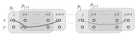
Figure 1. Intuition for points of increment and decrement

The left column indicates the two variables $x,y$ and the remaining columns indicate valuations. E.g., $\sigma(i+1)(y)=d$ and $\sigma(j+l+1)(x)=d^{\prime}$. Let $\mathit{fr}_{i}=\{\varphi^{\prime}\in\Omega^{\varphi}_{l}\mid\sigma,i\models\varphi^{\prime}\}$. We have indicated this pictorially by highlighting the valuations that determine the contents of $\mathit{fr}_{i}$. The data values for $x$ at positions $i$ and $(i+l+1)$ are equal, but the positions are too far apart to be captured by any one constraint of the form ${\sf X}^{\alpha}x\approx{\sf X}^{\beta}x$ in $\Omega^{\varphi}_{l}$. However, the intermediate position $(i+1)$ has the same data value and is less than $l$ positions apart from both positions. One constraint from $\Omega^{\varphi}_{l}$ can capture the data repetition between positions $i$ and $(i+1)$ while another one captures the repetition between positions $(i+1)$ and $(i+l+1)$, thus indirectly capturing the repetition between positions $i$ and $(i+l+1)$. For $e\in\{0,\ldots,l\}$, an $(e,\varphi)$-frame $\mathit{fr}$, $i\in\{0,\ldots,e\}$ and a variable $x$, we say that there is a forward (resp. backward) reference from $(x,i)$ in $\mathit{fr}$ if ${\sf X}^{i}x\approx{\sf X}^{i+j}y\in\mathit{fr}$ (resp. ${\sf X}^{i}x\approx{\sf X}^{i-j}y\in\mathit{fr}$) for some $j>0$ and $y\in\textit{DVARS}^{\varphi}$. The constraint $x\approx{\sf X}y$ in $\mathit{fr}_{i}$ above is a forward reference from $(x,0)$ in $\mathit{fr}_{i}$, while the constraint ${\sf X}^{l}x\approx y$ is a backward reference from $(x,l)$ in $\mathit{fr}_{i+1}$.

In Figure 1, the data values of $x$ at positions $j$ and $(j+l+1)$ are equal, but the two positions are too far apart to be captured by any constraint of the form ${\sf X}^{\alpha}z\approx{\sf X}^{\beta}w$ in $\Omega^{\varphi}_{l}$. Neither are there any intermediate positions with the same data value to capture the repetition indirectly. We maintain a counter to keep track of the number of such remote data repetitions. Let $X\subseteq\textit{DVARS}^{\varphi}$ be a set of variables. A point of decrement for counter $X$ in an $(e,\varphi)$-frame $\mathit{fr}$ is an equivalence class of the form ${[(x,e)]}_{\mathit{fr}}$ such that there is no backward reference from $(x,e)$ in $\mathit{fr}$ and ${\sf PO}_{\mathit{fr}}(x,e)=X$. In the above picture, the equivalence class ${[(x,l)]}_{\mathit{fr}_{j+1}}$ in the frame $\mathit{fr}_{j+1}$ is a point of decrement for $\{x\}$. A point of increment for $X$ in an $(l,\varphi)$-frame $\mathit{fr}$ is an equivalence class of the form ${[(x,0)]}_{\mathit{fr}}$ such that there is no forward reference from $(x,0)$ in $\mathit{fr}$ and ${[(x,0)]}_{\mathit{fr}}\cup{\sf PO}_{\mathit{fr}}(x,0)=X$. In the above picture, the equivalence class ${[(x,0)]}_{\mathit{fr}_{j}}$ in the frame $\mathit{fr}_{j}$ is a point of increment for $\{x\}$. Points of increment are not present in $(e,\varphi)$-frames for $e<l$ since such frames do not contain complete information about constraints in the next $l$ positions. We denote by $\mathit{inc}(\mathit{fr})$ the vector indexed by non-empty subsets of $\textit{DVARS}^{\varphi}$, where each coordinate contains the number of points of increment in $\mathit{fr}$ for the corresponding subset of variables. Similarly, we have the vector $\mathit{dec}(\mathit{fr})$ for points of decrement.

Intuitively, points of increment are positions where there is an opportunity to assign a value to variable $y$ in order to satisfy a data repetition constraint like $x\approx\Diamond^{-1}y$ that may occur later in a symbolic model. On the other hand, points of decrements are those positions of the symbolic models where we are obliged to ensure that some data value repeats in the past. So if there are lots of points of decrement, we have lots of obligations to repeat lots of data values in the past. If one needs to be able to do this, there should be lots of opportunities (points of increment) that have occured in the past. We can ensure that there are sufficient points of increment in the past by using counters — every time we see a point of increment along a symbolic model, we increment the counter. Every time we see a point of decrement, we decrement the counter. There will be sufficiently many points of increment to satisfy all the data repetition constraints if the value of the counter always stays above zero. This is exactly the constraint imposed on counters in energy games (the counter value is intuitively the “energy” stored in a system and it should never be below zero) and that’s why energy games are useful to solve LRV[$\top$, $\approx$, $\leftarrow$] games. Energy games are effectively equivalent to single-sided VASS games and we use the later since, technically, it is easier to adapt to our context. The value of a counter at a position maintains the number of points of increment before that position that are free to be used to satisfy constraints that may occur later. We give the formal construction below. The resulting single-sided VASS game is basically a product of two components. The first one is a deterministic parity automaton which checks whether a symbolic model symbolically satisfies the given LRV[$\top$, $\approx$, $\leftarrow$] formula. The second component is a VASS which keeps track of the number of points of increment and decrement. By playing two player games on these two components in parallel, we can determine whether system has a strategy to build a symbolic model that symbolically satisfies the given LRV[$\top$, $\approx$, $\leftarrow$] formula while, at the same time, ensuring that the symbolic model is realizable.

Given a LRV[$\top$, $\approx$, $\leftarrow$] formula $\varphi$ in which $(\textit{DVARS}^{e}\cap\textit{DVARS}^{\varphi})=\emptyset=(\textit{BVARS}^{s}\cap\textit{BVARS}^{\varphi})$, we construct a single-sided VASS game as follows. Let $l$ be the ${\sf X}$-length of $\varphi$ and ${\sf FR}$ be the set of all $(e,\varphi)$-frames for all $e\in\{0,\ldots,l\}$. Let $A^{\varphi}$ be a deterministic parity automaton that accepts a symbolic model iff it symbolically satisfies $\varphi$, with set of states $Q^{\varphi}$ and initial state $q^{\varphi}_{\mathit{init}}$. The single-sided VASS game will have set of counters $\mathcal{P}^{+}(\textit{DVARS}^{\varphi})$, set of environment states $\{-1,0,\ldots,l\}\times Q^{\varphi}\times({\sf FR}\cup\{\bot\})$ and set of system states $\{-1,0,\ldots,l\}\times Q^{\varphi}\times({\sf FR}\cup\{\bot\})\times\mathcal{P}(\textit{BVARS}^{\varphi})$. Every state will inherit the colour of its $Q^{\varphi}$ component. For convenience, we let $\bot$ to be the only $(-1,\varphi)$-frame and $(\bot,\mathit{fr}^{\prime})$ be one-step consistent for every $0$-frame $\mathit{fr}^{\prime}$. The initial state is $(-1,q^{\varphi}_{\mathit{init}},\bot)$, the initial counter values are all $0$ and the transitions are as follows ($\lceil\cdot\rceil l$ denotes the mapping that is identity on $\{-1,0,\ldots,l-1\}$ and maps all others to $l$).

• $(e,q,\mathit{fr})\xrightarrow{\vec{0}}(e,q,\mathit{fr},V)$ for every $e\in\{-1,0,\ldots,l\}$, $q\in Q^{\varphi}$, $\mathit{fr}\in{\sf FR}\cup\{\bot\}$ and $V\subseteq\textit{BVARS}^{\varphi}$.

• $(e,q^{\varphi}_{\mathit{init}},\mathit{fr},V)\xrightarrow{\mathit{inc}(\mathit{fr})-\mathit{dec}(\mathit{fr}^{\prime})}(e+1,q^{\varphi}_{\mathit{init}},\mathit{fr}^{\prime})$ for every $V\subseteq\textit{BVARS}^{\varphi}$, $e\in\{-1,0,\ldots,l-2\}$, $(e,\varphi)$-frame $\mathit{fr}$ and $(e+1,\varphi)$-frame $\mathit{fr}^{\prime}$, where the pair $(\mathit{fr},\mathit{fr}^{\prime})$ is one-step consistent and $\{p\in\textit{BVARS}^{\varphi}\mid{\sf X}^{e+1}p\in\mathit{fr}^{\prime}\}=V$.

• $(e,q,\mathit{fr},V)\xrightarrow{\mathit{inc}(\mathit{fr})-\mathit{dec}(\mathit{fr}^{\prime})}(\lceil e+1\rceil l,q^{\prime},\mathit{fr}^{\prime})$ for every $e\in\{l-1,l\}$, $(e,\varphi)$-frame $\mathit{fr}$, $V\subseteq\textit{BVARS}^{\varphi}$, $q,q^{\prime}\in Q^{\varphi}$ and $(\lceil e+1\rceil l,\varphi)$-frame $\mathit{fr}^{\prime}$, where the pair $(\mathit{fr},\mathit{fr}^{\prime})$ is one-step consistent, $\{p\in\textit{BVARS}^{\varphi}\mid{\sf X}^{\lceil e+1\rceil l}p\in\mathit{fr}^{\prime}\}=V$ and $q\xrightarrow{\mathit{fr}^{\prime}}q^{\prime}$ is a transition in ${A^{\varphi}}$.

Transitions of the form $(e,q,\mathit{fr})\xrightarrow{\vec{0}}(e,q,\mathit{fr},V)$ let the environment choose any subset $V$ of $\textit{BVARS}^{\varphi}$ to be true in the next round. In transitions of the form $(e,q,\mathit{fr},V)\xrightarrow{\mathit{inc}(\mathit{fr})-\mathit{dec}(\mathit{fr}^{\prime})}(\lceil e+1\rceil l,q^{\prime},\mathit{fr}^{\prime})$, the condition $\{p\in\textit{BVARS}^{\varphi}\mid{\sf X}^{\lceil e+1\rceil l}p\in\mathit{fr}^{\prime}\}=V$ ensures that the frame $\mathit{fr}^{\prime}$ chosen by the system is compatible with the subset $V$ of $\textit{BVARS}^{\varphi}$ chosen by the environment in the preceding step. By insisting that the pair $(\mathit{fr},\mathit{fr}^{\prime})$ is one-step consistent, we ensure that the sequence of frames built during a game is a symbolic model. The condition $q\xrightarrow{\mathit{fr}^{\prime}}q^{\prime}$ ensures that the symbolic model is accepted by $A^{\varphi}$ and hence symbolically satisfies $\varphi$. The update vector $\mathit{inc}(\mathit{fr})-\mathit{dec}(\mathit{fr}^{\prime})$ ensures that symbolic models are realizable, as explained in the proof of the following result.

Lemma 6 (repeating values to VASS).

Let $\varphi$ be a LRV$[\top$, $\approx$, $\leftarrow]$ formula with $(\textit{DVARS}^{e}\cap\textit{DVARS}^{\varphi})=\emptyset$ and $(\textit{BVARS}^{s}\cap\textit{BVARS}^{\varphi})=\emptyset$. Then system has a winning strategy in the corresponding single-sided LRV$[\top$, $\approx$, $\leftarrow]$ game iff she has a winning strategy in the single-sided VASS game constructed above.

Proof 5.1.

We begin with a brief description of the ideas used. A game on the single-sided VASS game results in a sequence of frames. The single-sided VASS game embeds automata which check that these sequences are symbolic models that symbolically satisfy $\varphi$. This in conjunction with Lemma 5 (symbolic vs. concrete models) will prove the result, provided the symbolic models are also realizable. Some symbolic models are not realizable since frames contain too many constraints about data values repeating in the past and no concrete model can satisfy all those constraints. To avoid this, the single-sided VASS game maintains counters for keeping track of the number of such constraints. Whenever a frame contains such a past repetition constraint that is not satisfied locally within the frame itself, there is an absence of backward references in the frame and it results in a point of decrement. Then the $-\mathit{dec}(\mathit{fr}^{\prime})$ part of transitions of the form $(e,q,\mathit{fr},V)\xrightarrow{\mathit{inc}(\mathit{fr})-\mathit{dec}(\mathit{fr}^{\prime})}(\lceil e+1\rceil l,q^{\prime},\mathit{fr}^{\prime})$ will decrement the corresponding counter. In order for this counter to have a value of at least $0$, the counter should have been incremented earlier by $\mathit{inc}(\mathit{fr})$ part of earlier transitions. This ensures that symbolic models resulting from the single-sided VASS games are realizable.

Now we give the details for the forward direction. Suppose the system player has a strategy $\mathit{ts}:\Upsilon^{*}\cdot\Upsilon^{e}\to\Upsilon^{s}$ in the single-sided LRV$[\top$, $\approx$, $\leftarrow]$ game. We will show that the system player has a strategy $\mathit{ss}:{(Q\times\mathbb{N}^{C})}^{*}\cdot(Q^{s}\times\mathbb{N}^{C})\to T$ in the single-sided VASS game. It is routine to construct such a strategy from the mapping $\mu:{(\mathcal{P}(\textit{BVARS}^{\varphi}))}^{*}\to{\sf FR}\cup\{\bot\}$ that we define now. For every sequence $\chi\in{(\mathcal{P}(\textit{BVARS}^{\varphi}))}^{*}$, we will define $\mu(\chi)$ and a concrete model of length $|\chi|$, by induction on $|\chi|$. For the base case $|\chi|=0$, the concrete model is the empty sequence and the frame is $\bot$.

For the induction step, suppose $\chi$ is of the form $\chi^{\prime}\cdot V$ and $\sigma$ is the concrete model defined for $\chi^{\prime}$ by induction hypothesis. Let $\upsilon^{e}:\textit{BVARS}^{e}\to\{\top,\bot\}$ be the mapping defined as $\upsilon^{e}(p)=\top$ iff $p\in V$. The system player’s strategy $\mathit{ts}$ in the single-sided LRV$[\top$, $\approx$, $\leftarrow]$ game will give a valuation $\mathit{ts}(\sigma\cdot\upsilon^{e})=\upsilon^{s}:\textit{DVARS}^{s}\to\mathbb{D}$. We define the finite concrete model to be $\sigma\cdot(\upsilon^{e}\oplus\upsilon^{s})$ and $\mu(\chi)$ to be the frame $\mathit{fr}^{\prime}=\{\varphi^{\prime}\in\Omega^{\varphi}_{l}\mid\sigma\cdot(\upsilon^{e}\oplus\upsilon^{s}),|\sigma|+1-\lceil|\sigma|\rceil l\models\varphi^{\prime}\}$.

Next we will prove that the strategy $\mathit{ss}$ defined above is winning for the system player. Suppose the system player plays according to $\mathit{ss}$ in the single-sided VASS game, resulting in the sequence of states

$$(-1,q^{\varphi}_{\mathit{init}},\bot)(-1,q^{\varphi}_{\mathit{init}},\bot,V_{1})(0,q^{\varphi}_{\mathit{init}},\mathit{fr}_{1})(0,q^{\varphi}_{\mathit{init}},\mathit{fr}_{1},V_{2})$$

$$(1,q^{\varphi}_{\mathit{init}},\mathit{fr}_{2})\cdots(l,q,\mathit{fr}_{l+1})(l,q,\mathit{fr}_{l+1},V_{l+2})(l,q^{\prime},\mathit{fr}_{l+2})\cdots$$

The sequence $\mathit{fr}_{l+1}\mathit{fr}_{l+2}\cdots$ is an infinite $(l,\varphi)$-symbolic model; call it $\rho$. It is clear from the construction that $\rho$ is realized by a concrete model $\sigma$, which is the result of the system player playing according to the winning strategy $\mathit{ts}$ in the LRV[$\top$, $\approx$, $\leftarrow$] game. So $\sigma,1\models\varphi$ and by Lemma 5 (symbolic vs. concrete models), $\rho$ symbolically satisfies $\varphi$. By definition of $A^{\varphi}$, the unique run of $A^{\varphi}$ on $\rho$ satisfies the parity condition and hence the play satisfies the parity condition in the single-sided VASS game. It remains to prove that if a transition given by $\mathit{ss}$ decrements some counter, that counter will have sufficiently high value. Any play starts with all counters having zero and a counter is decremented by a transition if the frame chosen by that transition has points of decrement for the counter. For $e\in\{1,\ldots,l+1\}$ and $x\in\textit{DVARS}^{\varphi}$, ${[(x,e)]}_{\mathit{fr}_{e}}$ cannot be a point of decrement in $\mathit{fr}_{e}$ — if it were, the data value $\sigma(e)(x)$ would have appeared in some position in $\{1,\ldots,e-1\}$, creating a backward reference from $(x,e)$ in $\mathit{fr}_{e}$.

For $i>l+1$, $x\in\textit{DVARS}^{\varphi}$ and $X\in\mathcal{P}^{+}(\textit{DVARS}^{\varphi})$, suppose ${[(x,l)]}_{\mathit{fr}_{i}}$ is a point of decrement for $X$ in $\mathit{fr}_{i}$. Before decrementing the counter $X$, it is incremented for every point of increment for $X$ in every frame $\mathit{fr}_{j}$ for all $j<i$. Hence, it suffices to associate with this point of decrement a point of increment for $X$ in a frame earlier than $\mathit{fr}_{i}$ that is not associated to any other point of decrement. Since ${[(x,l)]}_{\mathit{fr}_{i}}$ is a point of decrement for $X$ in $\mathit{fr}_{i}$, the data value $\sigma(i)(x)$ appears in some of the positions $\{1,\ldots,i-l-1\}$. Let $i^{\prime}=\max\{j\in\{1,\ldots,i-l-1\}\mid\exists y\in\textit{DVARS}^{\varphi},\sigma(j)(y)=\sigma(i)(x)\}$. Let $x^{\prime}\in X$ be such that $\sigma(i^{\prime})(x^{\prime})=\sigma(i)(x)$ and associate with ${[(x,l)]}_{\mathit{fr}_{i}}$ the class ${[(x^{\prime},0)]}_{\mathit{fr}_{i^{\prime}+l}}$, which is a point of increment for $X$ in $\mathit{fr}_{i^{\prime}+l}$. The class ${[(x^{\prime},0)]}_{\mathit{fr}_{i^{\prime}+l}}$ cannot be associated with any other point of decrement for $X$ — suppose it were associated with ${[(y,l)]}_{\mathit{fr}_{j}}$, which is a point of decrement for $X$ in $\mathit{fr}_{j}$. Then $\sigma(j)(y)=\sigma(i)(x)$. If $j=i$, then ${[(x,l)]}_{\mathit{fr}_{i}}={[(y,l)]}_{\mathit{fr}_{j}}$ and the two points of decrement are the same. So $j<i$ or $j>i$. We compute $j^{\prime}$ for ${[(y,l)]}_{\mathit{fr}_{j}}$ with $j^{\prime}<j$ just like we computed $i^{\prime}$ for ${[(x,l)]}_{\mathit{fr}_{i}}$. If $j<i$, then $j$ would be one of the positions in $\{1,\ldots,i-l-1\}$ where the data value $\sigma(i)(x)$ appears ($j$ cannot be in the interval $[i-l,i-1]$ since those positions do not contain the data value $\sigma(i)(x)$; if they did, there would have been a backward reference from $(x,l)$ in $\mathit{fr}_{i}$ and ${[(x,l)]}_{\mathit{fr}_{i}}$ would not have been a point of decrement), so $j\leq i^{\prime}$ (and hence $j^{\prime}<i^{\prime}$). If $j>i$, then $i$ is one of the positions in $\{1,\ldots,j-l-1\}$ where the data value $\sigma(j)(y)$ appears ($i$ cannot be in the interval $[j-l,j-1]$ since those positions do not contain the data value $\sigma(j)(y)$; if they did, there would have been a backward reference from $(y,l)$ in $\mathit{fr}_{j}$ and ${[(y,l)]}_{\mathit{fr}_{j}}$ would not have been a point of decrement), so $i\leq j^{\prime}$ (and hence $i^{\prime}<j^{\prime}$). In both cases, $j^{\prime}\neq i^{\prime}$ and hence, the class ${[y^{\prime},0]}_{\mathit{fr}_{j^{\prime}+l}}$ we associate with ${[(y,l)]}_{\mathit{fr}_{j}}$ would be different from ${[(x^{\prime},0)]}_{\mathit{fr}_{i^{\prime}+l}}$.

Next we give the details for the reverse direction. Suppose the system player has a strategy $\mathit{ss}:{(Q\times\mathbb{N}^{C})}^{*}\cdot(Q^{s}\times\mathbb{N}^{C})\to T$ in the single-sided VASS game. We will show that the system player has a strategy $\mathit{ts}:\Upsilon^{*}\cdot\Upsilon^{e}\to\Upsilon^{s}$ in the single-sided LRV$[\top$, $\approx$, $\leftarrow]$ game. For every $\sigma\in\Upsilon^{*}$ and every $\upsilon^{e}\in\Upsilon^{e}$, we will define $\mathit{ts}(\sigma\cdot\upsilon^{e}):\textit{DVARS}^{\varphi}\to\mathbb{D}$ and a sequence of configurations $\chi\cdot((e,q,\mathit{fr}),\vec{n}_{\mathit{inc}}-\vec{n}_{\mathit{dec}})$ in ${(Q\times\mathbb{N}^{C})}^{*}\cdot(Q^{e}\times\mathbb{N}^{C})$ of length $2|\sigma|+3$ such that for every counter $X\in\mathcal{P}^{+}(\textit{DVARS}^{\varphi})$, $\vec{n}_{\mathit{inc}}(X)$ is the sum of the number of points of increment for $X$ in all the frames occurring in $\chi$ and $\vec{n}_{\mathit{dec}}(X)$ is the sum of the number of points of decrement for $X$ in all the frames occurring in $\chi$ and in $\mathit{fr}$. We will do this by induction on $|\sigma|$ and prove that the resulting strategy is winning for the system player. By frames occurring in $\chi$, we refer to frames $\mathit{fr}$ such that there are consecutive configurations $((e,q,\mathit{fr}),\vec{n})((e,q,\mathit{fr},V),\vec{n})$ in $\chi$. By $\Pi_{{\sf FR}}(\chi)(i)$, we refer to $i$^th such occurrence of a frame in $\chi$. Let $\{d_{0},d_{1},\ldots\}\subseteq\mathbb{D}$ be a countably infinite set of data values.

For the base case $|\sigma|=0$, let $V\subseteq\textit{BVARS}^{e}$ be defined as $p\in V$ iff $\upsilon^{e}(p)=\top$. Let $\mathit{ss}(((-1,q^{\varphi}_{\mathit{init}},\bot),\vec{0})\cdot((-1,q^{\varphi}_{\mathit{init}},\bot,V),\vec{0}))$ be the transition $(-1,q^{\varphi}_{\mathit{init}},\bot,V)\xrightarrow{\vec{0}-\mathit{dec}(\mathit{fr}_{1})}(0,q,\mathit{fr}_{1})$. Since $\mathit{ss}$ is a winning strategy for system in the single-sided VASS game, $\mathit{dec}(\mathit{fr}_{1})$ is necessarily equal to $\vec{0}$. The set of variables $\textit{DVARS}^{\varphi}$ is partitioned into equivalence classes by the $(0,\varphi)$-frame $\mathit{fr}_{1}$. We define $\mathit{ts}(\upsilon^{e})$ to be the valuation that assigns to each such equivalence class a data value $d_{j}$, where $j$ is the smallest number such that $d_{j}$ is not assigned to any variable yet. We let the sequence of configurations be $((-1,q^{\varphi}_{\mathit{init}},\bot),\vec{0})\cdot((-1,q^{\varphi}_{\mathit{init}},\bot,V),\vec{0})\cdot((0,q,\mathit{fr}_{1}),-\mathit{dec}(\mathit{fr}_{1}))$.

For the induction step, suppose $\sigma\cdot\upsilon^{e}=\sigma^{\prime}\cdot(\upsilon^{e}_{1}\oplus\upsilon^{s}_{1})\cdot\upsilon^{e}$ and $\chi^{\prime}\cdot((e,q,\mathit{fr}),\vec{n})$ is the sequence of configurations given by the induction hypothesis for $\sigma^{\prime}\cdot\upsilon^{e}_{1}$. If $\{\varphi^{\prime}\in\Omega^{\varphi}_{l}\mid\sigma^{\prime}\cdot(\upsilon^{e}_{1}\oplus\upsilon^{s}_{1}),|\sigma^{\prime}|+1-e\models\varphi^{\prime}\}\neq\mathit{fr}$, it corresponds to the case where the system player in the LRV$[\top$, $\approx$, $\leftarrow]$ game has already deviated from the strategy we have defined so far. So in this case, we define $\mathit{ts}(\sigma\cdot\upsilon^{e})$ and the sequence of configurations to be arbitrary. Otherwise, we have $\{\varphi^{\prime}\in\Omega^{\varphi}_{l}\mid\sigma^{\prime}\cdot(\upsilon^{e}_{1}\oplus\upsilon^{s}_{1}),|\sigma^{\prime}|+1-e\models\varphi^{\prime}\}=\mathit{fr}$. Let $V\subseteq\textit{BVARS}^{e}$ be defined as $p\in V$ iff $\upsilon^{e}(p)=\top$ and let $\mathit{ss}(\chi^{\prime}\cdot((e,q,\mathit{fr}),\vec{n})\cdot((e,q,\mathit{fr},V),\vec{n}))$ be the transition $(e,q,\mathit{fr},V)\xrightarrow{\mathit{inc}(\mathit{fr})-\mathit{dec}(\mathit{fr}^{\prime})}(\lceil e+1\rceil l,q^{\prime},\mathit{fr}^{\prime})$. We define the sequence of configurations as $\chi^{\prime}\cdot((e,q,\mathit{fr}),\vec{n})\cdot((e,q,\mathit{fr},V)\vec{n})\cdot((\lceil e+1\rceil l,q^{\prime},\mathit{fr}^{\prime}),\vec{n}+\mathit{inc}(\mathit{fr})-\mathit{dec}(\mathit{fr}^{\prime}))$. Since $\mathit{ss}$ is a winning strategy for the system player in the single-sided VASS game, $\vec{n}+\mathit{inc}(\mathit{fr})-\mathit{dec}(\mathit{fr}^{\prime})\geq\vec{0}$. The valuation $\mathit{ts}(\sigma\cdot\upsilon^{e}):\textit{DVARS}^{\varphi}\to\mathbb{D}$ is defined as follows. The set $\textit{DVARS}^{\varphi}$ is partitioned by the equivalence classes at level $\lceil e+1\rceil l$ in $\mathit{fr}^{\prime}$. For every such equivalence class ${[(x,\lceil e+1\rceil l)]}_{\mathit{fr}^{\prime}}$, assign the data value $d^{\prime}$ as defined below.

1. If there is a backward reference ${\sf X}^{\lceil e+1\rceil l}x\approx{\sf X}^{\lceil e+1\rceil l-j}y$ in $\mathit{fr}^{\prime}$, let $d^{\prime}=\sigma^{\prime}\cdot(\upsilon^{e}_{1}\oplus\upsilon^{s}_{1})(|\sigma^{\prime}|+2-j)(y)$.

2. If there are no backward references from $(x,\lceil e+1\rceil l)$ in $\mathit{fr}^{\prime}$ and the set ${\sf PO}_{\mathit{fr}}(x,\lceil e+1\rceil l)$ of past obligations of $x$ at level $\lceil e+1\rceil l$ in $\mathit{fr}^{\prime}$ is empty, let $d^{\prime}$ be $d_{j}$, where $j$ is the smallest number such that $d_{j}$ is not assigned to any variable yet.

3. If there are no backward references from $(x,\lceil e+1\rceil l)$ in $\mathit{fr}^{\prime}$ and the set ${\sf PO}_{\mathit{fr}}(x,\lceil e+1\rceil l)$ of past obligations of $x$ at level $\lceil e+1\rceil l$ in $\mathit{fr}^{\prime}$ is the non-empty set $X$, then ${[(x,\lceil e+1\rceil l)]}_{\mathit{fr}^{\prime}}$ is a point of decrement for $X$ in $\mathit{fr}^{\prime}$. Pair off this with a point of increment for $X$ in a frame that occurs in $\chi^{\prime}\cdot((e,q,\mathit{fr}),\vec{n})\cdot((e,q,\mathit{fr},V),\vec{n})$ that has not been paired off before. It is possible to do this for every point of decrement for $X$ in $\mathit{fr}^{\prime}$, since $(\vec{n}+\mathit{inc}(\mathit{fr}))(X)$ is the number of points of increment for $X$ occurring in $\chi^{\prime}\cdot((e,q,\mathit{fr}),\vec{n})\cdot((e,q,\mathit{fr},V),\vec{n})$ that have not yet been paired off and $(\vec{n}+\mathit{inc}(\mathit{fr}))(X)\geq\mathit{dec}(\mathit{fr}^{\prime})(X)$. Suppose we pair off ${[(x,\lceil e+1\rceil l)]}_{\mathit{fr}^{\prime}}$ with a point of increment ${[(y,0)]}_{\mathit{fr}_{i}}$ in the frame $\mathit{fr}_{i}=\Pi_{{\sf FR}}(\chi^{\prime}\cdot((e,q,\mathit{fr}),\vec{n})\cdot((e,q,\mathit{fr},V),\vec{n}))(i)$, then let $d^{\prime}$ be $\sigma^{\prime}\cdot(\upsilon^{e}_{1}\oplus\upsilon^{s}_{1})(i)(y)$.

Suppose the system player plays according to the strategy $\mathit{ts}$ defined above, resulting in the model $\sigma=(\upsilon^{e}_{1}\oplus\upsilon^{s}_{1})\cdot(\upsilon^{e}_{2}\oplus\upsilon^{s}_{2})\cdots$. It is clear from the construction that there is a sequence of configurations

$$((-1,q^{\varphi}_{\mathit{init}},\bot),\vec{0})((-1,q^{\varphi}_{\mathit{init}},\bot,V_{1}),\vec{0})$$

$$((0,q^{\varphi}_{\mathit{init}},\mathit{fr}_{1}),\vec{n}_{1})((0,q^{\varphi}_{\mathit{init}},\mathit{fr}_{1},V_{2}),\vec{n}_{1})$$

$$((1,q^{\varphi}_{\mathit{init}},\mathit{fr}_{2}),\vec{n}_{2})\cdots((l,q,\mathit{fr}_{l+1}),\vec{n}_{l+1})$$

$$((l,q,\mathit{fr}_{l+1},V_{l+2}),\vec{n}_{l+1})((l,q^{\prime},\mathit{fr}_{l+2}),\vec{n}_{l+2})\cdots$$

that is the result of the system player playing according to the strategy $\mathit{ss}$ in the single-sided VASS game such that the concrete model $\sigma$ realizes the symbolic model $\mathit{fr}_{l+1}\mathit{fr}_{l+2}\cdots$. Since $\mathit{ss}$ is a winning strategy for the system player, the sequence of configurations above satisfy the parity condition of the single-sided VASS game, so $\mathit{fr}_{l+1}\mathit{fr}_{l+2}\cdots$ symbolically satisfies $\varphi$. From Lemma 5 (symbolic vs. concrete models), we conclude that $\sigma$ satisfies $\varphi$.

Corollary 7.

The winning strategy existence problem for single-sided LRV$[\top$, $\approx$, $\leftarrow]$ game of repeating values (without past-time temporal modalities) is in 3ExpTime.

Proof 5.2.

We recall from [9, Corollary 5.7] that the winning strategy existence problem for energy games (and hence single-sided VASS games) can be solved in time ${(|V|\cdot\parallel E\parallel)}^{2^{O(d\cdot\log(d+p))}}+O(d\cdot c)$, where $V$ is the set of vertices, $\parallel E\parallel$ is the maximal absolute value of counter updates in the edges, $d$ is the number of counters, $p$ is the number of even priorities and $c$ is the maximal value of the initial counter values. For a LRV$[\top$, $\approx$, $\leftarrow]$ formula $\varphi$ with $\textit{DVARS}^{e}\cap\textit{DVARS}^{\varphi}=\textit{BVARS}^{s}\cap\textit{BVARS}^{\varphi}=\emptyset$ and no past-time temporal modalities, a deterministic parity automaton for symbolic models can be constructed in 2ExpTime, having doubly exponentially many states. A frame is a subset of atomic constraints, so there are exponentially many frames. Hence, the number of vertices $|V|$ in the constructed single-sided VASS game is doubly exponential. The value of ${\parallel}E{\parallel}$ is polynomial, since it depends on the number of points of increment and the number of points of decrement in frames. The value of $p$ is bounded by the number of priorities used in the parity automaton and hence, it is at most doubly exponential. The value of $c$ is zero. The number of counters $d$ is exponential, since there is one counter for every subset of data variables used in $\varphi$. Hence, the upper bound for energy games translates to 3ExpTime for single-sided LRV$[\top$, $\approx$, $\leftarrow]$ games.

Our decidability proof thus depends ultimately on energy games, as hinted in the title of this paper. Next we show that single-sided VASS games can be effectively reduced to single-sided LRV[$\top$, $\approx$, $\leftarrow$] games.

Theorem 8.

Given a single-sided VASS game, a single-sided LRV[$\top$, $\approx$, $\leftarrow$] game can be constructed in polynomial time so that system has a winning strategy in the first game iff system has a winning strategy in the second one.

Proof 5.3.

We begin with a brief description of the ideas used. We will simulate runs of single-sided VASS games with models of formulas in LRV. The formulas satisfied at position $i$ of the concrete model will contain information about counter values before the $i$^th transition and the identity of the $i$^th transition chosen by the environment and the system players in the run of the single-sided VASS game. For simulating a counter $x$, we use two system variables $x$ and $\overline{x}$. The data values assigned to these variables from positions $1$ to $i$ in a concrete model $\sigma$ will represent the counter value that is equal to the cardinality of the set $\{d\in\mathbb{D}\mid\exists j\in\{1,\ldots,i\},\sigma(j)(x)=d,\forall j^{\prime}\in\{1,\ldots,i\},\sigma(j^{\prime})(\overline{x})\neq d\}$. Using formulas in LRV[$\top$, $\approx$, $\leftarrow$], the two players can be enforced to correctly update the concrete model to faithfully reflect the moves in the single-sided VASS game. A formula can also be written to ensure that system wins the single-sided LRV[$\top$, $\approx$,$\leftarrow$] game iff the single-sided VASS game being simulated satisfies the parity condition.

Now we give the details. Given a single-sided VASS game, we will make the following assumptions about it without loss of generality.

• The initial state belongs to the environment player (if it doesn’t, we can add an extra state and a transition to achieve this).

• The environment and system players strictly alternate (if there are transitions between states belonging to the same player, we can add a dummy state belonging to the other player in between).

• The initial counter values are zero (if they aren’t, we can add extra transitions before the initial state and force the system player to get the counter values from zero to the required values).

The formula giving the winning condition of the single-sided LRV[$\top$, $\approx$, $\leftarrow$] game is made up of the following variables. Suppose $T^{e}$ and $T^{s}$ are the sets of environment and systems transitions respectively. For every transition $t\in T^{e}$, there is an environment variable $p_{t}$. We indicate that the environment player chooses a transition $t$ by setting $p_{t}$ to true. For every transition $t\in T^{s}$ of the single-sided VASS game, there is a system variable $t$. There is a system variable $\mathit{c}t_{s}$ to indicate the moves made by the system player. We indicate that the system player chooses a transition $t$ by mapping $t$ and $\mathit{c}t_{s}$ to the same data value. For every counter $x$ of the single-sided VASS game, there are system variables $x$ and $\overline{x}$.

The formula $\varphi_{e}$ indicates that the environment player makes some wrong move and it is the disjunction of the following formulas.

• The environment does not choose any transition in some round.

  $$F(~{}\bigwedge_{t\in T^{e}}\lnot p_{t}~{})$$

• The environment chooses more than one transition in some round.

  $$F(~{}\bigvee_{t\neq t^{\prime}\in T^{e}}(p_{t}\land p_{t^{\prime}})~{})$$

• The environment does not start with a transition originating from the designated initial state.

  $$\bigvee_{t\in T^{e},\text{ origin of }t\text{ is not the initial state}}p_{t}$$

• The environment takes some transition that cannot be taken after the previous transition by the system player.

  $$\bigvee_{t\in T^{s}}F(~{}t\approx\mathit{c}t_{s}~{}\land\bigwedge_{t^{\prime}\in T_{s}\setminus\{t\}}\lnot(t^{\prime}\approx\mathit{c}t_{s})~{}\land$$

  $$~{}\bigvee_{t^{\prime}\in T^{e},~{}t^{\prime}\text{ can not come after }t}{\sf X}(p_{t^{\prime}})~{})$$

For simulating a counter $x$, we use two variables $x$ and $\overline{x}$. The data values assigned to these variables from positions $1$ to $i$ in a concrete model $\sigma$ will represent the counter value that is equal to the cardinality of the set $\{d\in\mathbb{D}\mid\exists j\in\{1,\ldots,i\},\sigma(j)(x)=d,\forall j^{\prime}\in\{1,\ldots,i\},\sigma(j^{\prime})(\overline{x})\neq d\}$. We will use special formulas for incrementing, decrementing and retaining previous values of counters.

• To increment a counter represented by $x,\overline{x}$, we force the next data values of $x$ and $\overline{x}$ to be new ones that have never appeared before in $x$ or $\overline{x}$.

  $$\varphi_{\mathit{inc}}(x,\overline{x})={\sf X}\lnot( ~{}(x\approx\Diamond^{-1}x)~{}\lor~{}(x\approx\Diamond^{-1}\overline{x})~{}\lor~{}(\overline{x}\approx\Diamond^{-1}x)~{}\lor~{}$$

  $$~{}(\overline{x}\approx\Diamond^{-1}\overline{x})~{}\lor~{}(x\approx\overline{x})~{})$$

• To decrement a counter represented by $x,\overline{x}$, we force the next position to have a data value for $x$ and $\overline{x}$ such that it has appeared in the past for $x$ but not for $\overline{x}$.

  $$\varphi_{\mathit{dec}}(x,\overline{x})= {\sf X}(~{}x\approx\overline{x}~{}\land~{}x\approx\Diamond^{-1}x~{}\land~{}\lnot(x\approx\Diamond^{-1}\overline{x})~{})$$

• To ensure that a counter represented by $x,\overline{x}$ is not changed, we force the next position to have a data value for $x$ that has already appeared in the past for $x$ and we force the next position to have a data value for $\overline{x}$ that has never appeared in the past for $x$ or $\overline{x}$.

  $$\varphi_{\mathit{nc}}(x,\overline{x})={\sf X}(~{}x\approx\Diamond^{-1}x~{}\land~{}\lnot(\overline{x}\approx\Diamond^{-1}x)~{}\land~{}\lnot(\overline{x}\approx\Diamond^{-1}\overline{x})~{})$$

The formula $\varphi_{s}$ indicates that the system player makes all the right moves and it is the conjunction of the following formulas.

• The system player always chooses at least one move.

  $$G(~{}\bigvee_{t\in T^{s}}t\approx\mathit{c}t_{s}~{})$$

• The system player always chooses at most one move.

  $$G(~{}\bigwedge_{t\neq t^{\prime}\in T^{s}}\lnot(t\approx\mathit{c}t_{s}\land t^{\prime}\approx\mathit{c}t_{s})~{})$$

• The system player always chooses a transition that can come after the previous transition chosen by the environment.

  $$\bigwedge_{t\in T^{e}}G(~{}p_{t}~{}\Rightarrow~{}\bigvee_{t^{\prime}\in T_{s},~{}t^{\prime}\text{ can come after }t}t^{\prime}\approx\mathit{c}t_{s}~{})$$

• The system player sets the initial counter values to zero.

  $$\bigwedge_{x\text{ is a counter}}x\approx\overline{x}$$

• The system player updates the counters properly.

  $$G(~{} \bigwedge_{(q,x++,q^{\prime})=t\in T^{s}}(~{}t\approx\mathit{c}t_{s}~{}\Rightarrow~{}\varphi_{\mathit{inc}}(x,\overline{x})~{}\land\bigwedge_{x^{\prime}\neq x}\varphi_{\mathit{nc}}(x^{\prime},\overline{x^{\prime}}))$$

  $$\bigwedge_{(q,\mathit{nop},q^{\prime})=t\in T^{s}}(~{}t\approx\mathit{c}t_{s}~{}\Rightarrow~{}\bigwedge_{x\text{ is a counter}}\varphi_{\mathit{nc}}(x,\overline{x})~{})$$

  $$\bigwedge_{(q,x--,q^{\prime})=t\in T^{s}}(~{}t\approx\mathit{c}t_{s}~{}\Rightarrow~{}\varphi_{\mathit{dec}}(x,\overline{x})~{}\land\bigwedge_{x^{\prime}\neq x}\varphi_{\mathit{nc}}(x^{\prime},\overline{x^{\prime}}))~{})$$

• The maximum colour occurring infinitely often is even.

  $$\bigvee_{j\text{ is an even colour}}GF(\bigvee_{t\in T^{e},\text{origin of }t\text{ has colour }j}(p_{t})$$

  $$\lor\bigvee_{t\in T^{s},\text{origin of }t\text{ has colour }j}(t\approx\mathit{c}t_{s}))~{}\land$$

  $$FG(\bigwedge_{t\in T,\text{ origin of }t\text{ has colour greater than }j}\lnot(p_{t}\lor t\approx\mathit{c}t_{s}))$$

The system player wins if the environment player makes any mistake or the system player makes all the moves correctly and satisfies the parity condition. We set the winning condition for the system player in the single-sided LRV[$\top$, $\approx$, $\leftarrow$] game to be $\varphi_{e}\lor\varphi_{s}$. If the system player has a winning strategy in the single-sided VASS game, the system player simply makes choices in the single-sided LRV[$\top$, $\approx$, $\leftarrow$] game to imitate the moves in the single-sided VASS game. Since the resulting concrete model satisfies $\varphi_{e}\lor\varphi_{s}$, the system player wins. Conversely, suppose the system player has a winning strategy in the single-sided LRV[$\top$, $\approx$, $\leftarrow$] game. In the case where the environment does not make any mistake, the system player has to choose data values such that the simulated sequence of states of the VASS satisfy the parity condition. Hence, the system player in the single-sided VASS game can follow the strategy of the system player in the single-sided LRV[$\top$, $\approx$, $\leftarrow$] game and irrespective of how the environment player plays, the system player wins.

6. Single-sided LRV[$\top$, $\approx$, $\rightarrow$] is undecidable

In this section we show that the positive decidability result for the single-sided LRV[$\top,\leftarrow$] game cannot be replicated for the future demands fragment, even in a restricted setting.

Theorem 9.

The winning strategy existence problem for single-sided LRV$[\top,\approx,\rightarrow]$ games is undecidable, even when the formula giving the winning condition uses one Boolean variable belonging to environment and three data variables belonging to system.

We don’t know the decidability status for the case where the formula uses less than three data variables belonging to system.

First we explain why the technique used for proving decidability in Section 5 cannot be applied here. In Section 5, atomic constraints can only test if a current data value appeared in the past. At any point of a game, system can satisfy such an atomic constraint by looking at data values that have appeared in the past and assigning such a data value to some variable in the current position of the game. However, this cannot be done when atomic constraints can refer to repetitions in the future — if system decides to satisfy such an atomic constraint at some point in the game, then system will be obligated to repeat a data value at some point in the future. The opponent environment can prevent this, if the formula specifying the winning condition for system is cleverly set up so that as soon as system commits itself to repeating some value in the future, it will not be able to make the repetition. Indeed, in this section, we use such formulas to force system to faithfully simulate a 2-counter machine — the formulas are set up so that if system makes a mistake in the simulation, he will have to commit to repeating some value in the future, and environment will not let the repetition happen, thus defeating system.

As in the previous undecidability results in Section 4, Theorem 9 is proven by a reduction from the reachability problem for 2-counter machines. System makes use of labels to encode the sequence of transitions of a witnessing run of the counter machine. This time, system uses 3 data variables $x,y,z$ (in addition to a number of Boolean variables which encode the labels); and environment uses just one Boolean variable $b$. Variables $x$, $y$ are used to encode the counters $c_{x}$ and $c_{y}$ as before, and variables $z$, $b$ are used to ensure that there are no ‘illegal’ transitions — namely, no decrements of a zero-valued counter, and no tests for zero for a non-zero-valued counter.

Each transition in the run of the 2-counter machine will be encoded using two consecutive positions of the game. Concretely, while in the previous coding of Section 4 a witnessing reachability run $t_{1}\,t_{2}\dotsb t_{n}\in\delta^{*}$ was encoded with the label sequence $\textit{begin}\,t_{1}\,t_{2}\dotsb t_{n}\hat{t}^{\omega}$, in this encoding transitions are interspersed with a special bis label, and thus the run is encoded as $t_{1}\textit{bis}\,t_{2}\,\textit{bis}\dotsb t_{n}\,\textit{bis}\,{(\hat{t}\,\textit{bis})}^{\omega}\in{(\delta\cup\{\textit{bis}\})}^{\omega}$.

Suppose a position has the label of a $c_{x}++$ instruction and the variable $x$ has the data value $d$. Our encoding will ensure that if the data value $d$ repeats in the future, it will be only once and at a position that has the label of a $c_{x}--$ instruction. A symmetrical property holds for $c_{y}$ and variable $y$. The value of counter $c_{x}$ (resp. $c_{y}$) before the $i^{\text{th}}$ transition (encoded in the $2i^{\textit{th}}$ and ${(2i+1)}^{\textit{st}}$ positions) is the number of positions $j<2i$ satisfying the following two conditions: (i) the position $j$ should have the label of a $c_{x}++$ instruction and (ii) $\sigma(j)(x)\not\in\{\sigma(j^{\prime})(x)\mid j+1<j^{\prime}<2i\}$. Intuitively, if $2i$ is the current position, the value of $c_{x}$ (resp. $c_{y}$) is the number of previous positions that have the label of a $c_{x}++$ instruction whose data value is not yet matched by a position with the label of a $c_{x}--$ instruction. In this reduction we assume that system plays first and environment plays next at each round, since it is easier to understand (the reduction also holds for the game where turns are inverted by shifting environment behavior by one position). At each round, system will play a label bis if the last label played was an instruction. Otherwise, she will choose the next transition of the 2-counter machine to simulate and she will chose the values for variables $x$, $y$, $z$ in such a way that the aforementioned encoding for counters $c_{x}$ and $c_{y}$ is preserved. To this end, system is bound by the following set of rules, described here pictorially:

The first (leftmost) rule, for example, reads that whenever there is a $c_{x}++$ transition label, then all four values for $x$ and $y$ in both positions (i.e., the instruction position and the next bis position) must have the same data value $d$ (which we call ‘principal’), which does not occur in the future under variable $y$. The third rule says that $c_{x}--$ is encoded by having $x$ on the first position to carry the ‘principal’ data value $d$ of the instruction, which is final (that is, it is not repeated in the future under $x$ or $y$), and all three remaining positions have the same data value $d^{\prime}$ different from $d$. In this way, system can make sure that the value of $c_{x}$ is decremented, by playing a data value $d$ that has occurred in a $c_{x}++$ position that is not yet matched. (While system could also play some data value which does not match any previous $c_{x}++$ position, this ‘illegal’ move leads to a losing play for system, as we will show.) In this rule, the fact that one transition of the $2$-counter machine is encoded using two positions of the game is used to ensure that the data value $d^{\prime}$ of $y$ (for which $d^{\prime}\neq d$) appears in the future both in $x$ and $y$. Thus, the presence of $d^{\prime}$ doesn’t affect the value of $c_{y}$ or $c_{x}$ —to affect either, the data value should repeat in only one variable. If we do not force $d^{\prime}$ to repeat in both variables in the future, this position can potentially be treated as an increment for $c_{y}$. Using two positions per transitions is a simple way of preventing this.

From these rules, it follows that every $c_{k}++$ can be matched to at most one future $c_{k}--$. However, there can be two ways in which this coding can fail: (a) there could be invalid tests $c_{k}=0?$, that is, a situation in which the preceding positions of the test contain a $c_{k}++$ instruction which is not matched with a $c_{k}--$ instruction; and (b) there could be some $c_{k}--$ with no previous matching $c_{k}++$. As we will see next, variables $z$ and $b$ play a crucial role in the game whenever any of these two cases occurs. In all the rounds, environment always plays $\top$, except if he detects that one of these two situations, (a) or (b), have arisen, in which case he plays $\bot$. In the following rounds system plays a value in $z$ that will enable to test, with an LRV formula, if there was indeed an (a) or (b) situation, in which case system will lose, or if environment was just ‘bluffing’, in which case system will win. Since this is the most delicate point in the reduction, we dedicate the remaining of this section to the explanation of how these two situations (a) and (b) are treated.

Remember that environment has just one bit of information to play with. The LRV property we build ensures that the sequence of $b$-values must be from the set $\top^{*}\bot^{*}\top^{\omega}$.

(a) Avoiding illegal tests for zero.

Suppose that at some point of the $2$-counter machine simulation, system decides to play a $c_{k}=0?$ instruction. Suppose there is some preceding $c_{k}++$ instruction for which either: (a1) there is no matching $c_{k}--$ instruction; or (a2) there is a matching $c_{k}--$ instruction but it occurs after the $c_{k}=0?$ instruction. Situation a1 can be easily avoided by ensuring that any winning play must satisfy the formula $\mu={\sf G}(\tau_{(c_{k}++)}\land{\sf F}\tau_{(c_{k}=0?)}\Rightarrow k\approx\Diamond k)$ for every $k\in\{x,y\}$. Here, $\tau_{inst}$ tests if the current position is labelled with an instruction of type $inst$. On the other hand, Situation a2 requires environment to play a certain strategy (represented in Figure 2-a2).

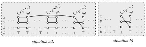
Figure 2. Depiction of best strategies in both situations.

This means that $c_{k}$ is non-zero at the position of the $c_{k}=0?$ instruction, and that this is an illegal transition; thus, environment must respond accordingly. Further, suppose this is the first illegal transition that has occurred so far. Environment, who so far has been playing only $\top$, decides to play $\bot$ to mark the cheating point. Further, he will continue playing $\bot$ until the matching $c_{k}--$ instruction is reached (if it is never reached, it is situation a1 and system loses as explained before), after which he will play $\top$ forever afterwards. In some sense, environment provides a link between the illegal transition and the proof of its illegality through a $\bot^{*}$-path. The following characterizes environment’s denouncement of an illegal test for zero:

Property 1: $b$ becomes $\bot$ at a $c_{k}=0?$ position and stops being $\bot$ at a $c_{k}--$ position thereafter.

Note that Property 1 is clearly definable by a formula $\pi_{1}$ of LRV$[\top,\approx,\rightarrow]$. If Property 1 holds, a formula $\varphi_{1}$ can constrain system to play $z$ according to the following: $z$ always carries the same data value, distinct from the values of all other variables, but as soon as the last $\bot$ value is played, which has to be on a $c_{k}--$ position, the value of $z$ changes and holds the principal value of that $c_{k}--$ instruction, and it continues to hold that value forever after (cf. Figure 2-$a2$). Further, if environment cheated in his denouncement by linking a $c_{k}=0?$ instruction with a future $c_{k}--$ with a matching $c_{k}++$ that falls in-between the test for zero and the decrement, then a property $\pi^{\prime}_{1}$ can catch this: there exists a $c_{k}++$ with $\bot$ whose principal value matches that of a future $z$-value.

Finally, assuming environment correctly denounced an illegal test for zero and system played accordingly on variable $z$, a property $\varphi^{\prime}_{1}$ can test that environment exposed an illegal transition, by testing that there exists a $c_{k}++$ instruction whose principal value corresponds to the $z$-value of some future position. Thus, the encoding for this situation is expressed with the formula $\psi_{1}=\mu\land((\pi_{1}\land\lnot\pi^{\prime}_{1})\Rightarrow(\varphi_{1}\land\lnot\varphi^{\prime}_{1}))$.

(b) Avoiding illegal decrements.

Suppose now that at some point of the $2$-counter machine simulation, system decides to play a $c_{k}--$ instruction for which there is no preceding $c_{k}++$ instruction matching its final data value. This is a form of cheating, and thus environment should respond accordingly. Further, suppose this is the first cheating that has occurred so far. Environment, who so far has been playing only $\top$, decides then to mark this position with $\bot$; and for the remaining of the play environment plays only $\top$ (even if more illegal transitions are performed in the sequel). Summing up, for this situation environment’s best strategy has a value sequence from $\top^{*}\bot\top^{\omega}$, and this property characterizes environment’s denouncement of an illegal decrement (cf. Figure 2-$b$).

Property 2: $b$ becomes $\bot$ at a $c_{k}--$ position and stops being $\bot$ immediately after.

A formula $\pi_{2}$ can test Property 2; and a formula $\varphi_{2}$ can constrain variable $z$ to always have the same data value —distinct from all other data values played on variables $x,y$— while $b$ contains $\top$ values; and as soon as $b$ turns to $\bot$ on a $c_{k}--$ position, then $z$ at the next position takes the value of the current variable $k$, and maintains that value (cf. Figure 2-$b$). Further, a formula $\varphi^{\prime}_{2}$ tests that in this case there must be some $c_{k}++$ position with a data value equal to variable $z$ of a future position. The formula corresponding to this case is then $\psi_{2}=\pi_{2}\Rightarrow\varphi_{2}\land\varphi^{\prime}_{2}$.

The final formula to test is then of the form $\varphi=\varphi_{\textit{lab}}\land\varphi_{x,y}\land\psi_{1}\land\psi_{2}$, where $\varphi_{\textit{lab}}$ ensures the finite-automata behavior of labels, and in particular that a final state can be reached, and $\varphi_{x,y}$ asserts the correct behavior of the variables $x,y$ relative to the labels. It follows that system has a winning strategy for the game with input $\varphi$ if, and only if, there is a positive answer to the reachability problem for the 2-counter machine. Finally, labels can be eliminated by means of special data values encoding blocks exactly as done in Section 4.2, and in this way Theorem 9 follows.

Proof 6.1 (Proof of Theorem 9).

We briefly discuss why the properties $\varphi_{\textit{lab}}$, $\varphi_{x,y}$, $\psi_{1}$ and $\psi_{2}$ can be described in LRV$[\top,\approx,\rightarrow]$.

Encoding $\varphi_{\textit{lab}}$ using some Boolean variables belonging to system is easy since it does not involve the use of data values.

The formula $\varphi_{x,y}$ can be encoded as ${\sf G}(\bigwedge_{a\in A}\tau_{a}\Rightarrow\zeta_{a})$ for $A=\{c_{x}++,c_{x}--,c_{x}=0?,c_{y}++,c_{y}--,c_{y}=0?\}$ and

$$\tau_{a}=\bigvee_{q,q^{\prime}\in Q,(q,a,q^{\prime})\in\delta}\lambda_{(q,a,q^{\prime})},$$

where $\lambda_{(q,a,q^{\prime})}$ tests that we are standing on a position labelled with instruction $(q,a,q^{\prime})$ (in particular not a bis position). Finally, $\zeta_{a}$ encodes the rules as already described. That is,

$$\zeta_{c_{x}++}={} x\approx y\land x\approx{\sf X}x\land y\approx{\sf X}y\land\lnot{\sf X}(x\approx\Diamond y),$$

$$\zeta_{c_{x}--}={} \lnot x\approx y\land\lnot x\approx\Diamond x\land\lnot x\approx\Diamond y\land y\approx{\sf X}y\land y\approx{\sf X}x,$$

$$\zeta_{c_{x}=0?}={} x\approx y\land x\approx{\sf X}x\land y\approx{\sf X}y,$$

and similarly for the rules on $c_{y}$.

The formula $\psi_{1}=\mu\land((\pi_{1}\land\lnot\pi^{\prime}_{1})\Rightarrow(\varphi_{1}\land\lnot\varphi^{\prime}_{1}))$ is actually composed of two conjunctions $\psi_{1}=\psi_{1}^{x}\land\psi_{1}^{y}$, one for $k=x$ and another for $k=y$, let us first suppose that $k=x$. Then,

• $\pi_{1}$, which checks Property 1, which is simply

  $$\pi_{1}=b{\sf U}(\lnot b\land\tau_{c_{x}=0?}\land{\sf X}(\lnot b{\sf U}\tau_{c_{x}--}))$$

• $\pi^{\prime}_{1}$, expresses that there exists a $c_{x}++$ with $\lnot b$ with value matching that of a future $z$-value:

  $$\pi^{\prime}_{1}={\sf F}(\tau_{c_{x}++}\land\lnot b\land x\approx\Diamond z)$$

• $\varphi_{1}$, on the other hand, checks that $z$ carries always the same data value, disjoint from the values of all other variables, but as soon as the last $\bot$ value is played the value of $z$ in the next position changes and holds now the $x$ value of that position, and it continues to hold it forever:

  $$\varphi_{1}={} \lnot(z\approx\Diamond x\lor z\approx\Diamond y)\land(z\approx{\sf X}z){\sf U}\big{(}\lnot(z\approx{\sf X}z)\land\lnot b\land{\sf X}b\land x\approx{\sf X}z\land{\sf X}{\sf G}(z\approx{\sf X}z)\big{)}$$

• finally, $\varphi^{\prime}_{1}$ tests there exists a $c_{x}++$ instruction whose principal value corresponds to the $z$-value of some future position:

  $$\varphi^{\prime}_{1} ={\sf F}(\tau_{c_{x}++}\land x\approx\Diamond z).$$

The formula $\psi_{2}=\pi_{2}\Rightarrow\varphi_{2}\land\varphi^{\prime}_{2}$ is also composed of two conjuncts, one for $k=x$ and one for $k=y$, let us only show the case $k=x$. Then,

• $\pi_{2}$ checks Property 2:

  $$\pi_{2}=b{\sf U}(\lnot b\land\tau_{c_{x}--}\land{\sf X}({\sf G}b))$$

• $\varphi_{2}$ checks that as soon as $b$ turns to $\bot$ then $z$ at the next position takes the value as current variable $x$, and maintains that value:

  $$\varphi_{2}={} \lnot(z\approx\Diamond x\lor z\approx\Diamond y)\land(z\approx{\sf X}z){\sf U}\big{(}\lnot(z\approx{\sf X}z)\land\lnot b\land x\approx{\sf X}z\land{\sf X}{\sf G}(z\approx{\sf X}z)\big{)}$$

• finally, $\varphi^{\prime}_{2}$ tests that in this situation there must be some $c_{x}++$ position with a data value equal to variable $z$ of a future position:

  $$\varphi^{\prime}_{2} ={\sf F}(\tau_{c_{x}++}\land x\approx\Diamond z).$$

Correctness.

Suppose first that the $2$-counter machine has an accepting run of the form $(q_{0},I_{1},q_{1})\dotsb(q_{n-1},I_{n},q_{n})$ with $q_{n}=q_{f}$. System’s strategy is then to play (the encoding of) the labels

$$(q_{0},I_{1},q_{1})\,\textit{bis}\,\dotsb(q_{n-1},I_{n},q_{n})\,\textit{bis}\,{(\hat{t}\,\textit{bis})}^{\omega}.$$

In this way, the formula $\varphi_{\textit{lab}}$ holds.

With respect to the data values on $x,y$, system will respect the rules depicted in Section 6, making $\varphi_{x,y}$ true.

Finally, system will play a data value in $z$ that at the beginning will be some data value which is not used on variables $x$ nor $y$. She will keep this data value all the time, but keeping an eye on the value of $b$ that is being played by environment. If environment plays a first $\bot$ on a $c_{k}--$ instruction, system will then play on $z$, at the next round, the data value of variable $k$ at this round. If environment plays a first $\bot$ at a $c_{k}=0?$ instruction and a last $\bot$ at a $c_{k}--$ instruction, again system will change the value of $z$ to have the principal value of the $c_{k}--$ instruction. In this way, system is sure to make true the formula $\varphi_{1}\land\lnot\varphi_{1}^{\prime}$ in one case, and formula $\varphi_{2}\land\varphi^{\prime}_{2}$ in the other case. All other cases for $b$ are going to be winning situations for system due to the preconditions $\pi_{1}\land\lnot\pi^{\prime}_{1}$ and $\pi_{2}$ in the formulas $\psi_{1}$ and $\psi_{2}$.

On the other hand, if there is no accepting run for the $2$-counter machine, then each play of system on variables $x,y$ and the variables verifying both $\varphi_{\textit{lab}}$ and $\varphi_{x,y}$ must have an illegal transition of type (a) or (b). At the first illegal transition environment will play $\bot$. If it is an illegal transition with the instruction $c_{k}--$, then environment will continue playing $\top$ in subsequent positions; if it is an illegal transition with the instruction $c_{k}=0?$, then environment will keep playing $\bot$ until the corresponding $c_{k}--$ matching to a witnessing $c_{k}++$ played before the $c_{k}=0?$ instruction is reached. In either of these situations the antecedent of $\psi_{1}$ or $\psi_{2}$ will be true while the consequent will be false; and thus the final formula will not hold, making system incapable of finding a winning strategy.

Finally, let us explain further how this reduction can be turned into a reduction for the game in which environment plays first and system plays second at each round. For the final formula $\varphi$ of the reduction, let $\varphi^{\prime}$ be the formula in which environment conditions are shifted one step to the right. This is simply done by replacing every sub-expression of the form ${\sf X}^{i}b$ with ${\sf X}^{i+1}b$. It follows that if environment starts playing $\top$ and then continues the play reacting to system strategy in the same way as before, system will have no winning strategy if, and only if, system had no winning strategy in the game where the turns are inverted.

Now we explain why the technique used to prove undecidability in this section cannot be used in Section 5. The crucial dependency on atomic constraints checking for repetition in the future occurs in avoiding illegal tests for zero and avoiding illegal decrements. For avoiding either of the errors, we let environment win by using atomic constraints that specify that the data value in the error position repeats in the future. Without the ability to test for repetition of values in the future, such a strategy for catching errors in simulation will not work. Indeed, the decidability result of Section 5 implies that with atomic constraints that can only test repetition of values in the past in system variables, counter machines cannot be simulated.

7. Single-sided LRV[$\langle{\sf X}^{-1},{\sf S}\rangle$, $\approx$, $\leftarrow$] is decidable

In this section, we prove that if we restrict nested formulas to use only past temporal operators and only allow past obligations, then single sided games are decidable. We enrich symbolic models used in Section 5 with information related to nested formulas and reduce the winning strategy existence problem to the same problem in single-sided VASS games.

The main idea is same as the one used in Section 5. We use symbolic models to ignore the special semantics of constraints like $x\approx\Diamond^{-1}y$ and treat such constraints like Boolean atomic propositions, whose truth value doesn’t depend on past positions. However, now we can have constraints of the form $x\approx\langle\psi?\rangle^{-1}y$, which says that the current data value assigned to $x$ should have been assigned to $y$ in some past position, and that past position should satisfy the formula $\psi$. Instead of tracking the number of points of decrement for the set $\{y\}$, we now track the number of points of decrement for the set of pairs $\{(y,\psi)\}$. We formalize this in the next two paragraphs.

For the rest of this section, we fix a LRV[$\langle{\sf X}^{-1},{\sf S}\rangle$, $\approx$, $\leftarrow$] formula $\varphi$. Let $\textit{BVARS}^{\varphi}\subseteq\textit{BVARS}$ and $\textit{DVARS}^{\varphi}\subseteq\textit{DVARS}$ be the set of Boolean and data variables used in $\varphi$. Let $\Phi$ be the set $\{\psi\mid\exists x,y\in\textit{DVARS}^{\varphi}\text{ s.t.~{}}x\approx\langle\psi?\rangle^{-1}y\text{ is a sub-formula in }\varphi\}\cup\{\top\}$. Intuitively, $\Phi$ is the set of formulas used as nested formulas inside $\varphi$. We will need to keep track of positions in the past where a data value repeats and the formulas in $\Phi$ that are satisfied at those positions. Formally, this is done by a repetition history, which is a subset of $\mathcal{P}(\textit{DVARS}^{\varphi})\times\mathcal{P}(\Phi)$. Intuitively, every element of a repetition history corresponds to one position in the past where a data value repeats. For example, the repetition history $\{(\{x,y\},\{\psi_{1},\psi_{2}\}),(\{y,z\},\{\psi_{2},\psi_{3}\})\}$ indicates that a data value repeats at two positions in the past. The first position satisfies $\psi_{1}$ and $\psi_{2}$ and at this position, the data value is assigned to variables $x$ and $y$. The second position satisfies $\psi_{2}$ and $\psi_{3}$ and at this position, the data value is assigned to variables $y$ and $z$. We denote the set of all repetition histories by $\mathit{RH}$.

We will also need to keep track of the variables in which a data value is required to be repeated, and the nested formulas that need to be satisfied at the positions where the repetitions happen. Formally, this is done by a past obligation, which is a subset of $\textit{DVARS}^{\varphi}\times\Phi$. For example, the past obligation $\{(y,\psi_{1}),(x,\psi_{2}),(x,\psi_{1}),(y,\psi_{2}),(y,\psi_{3}),(z,\psi_{3}),(z,\psi_{2})\}$ indicates that a data value needs to be repeated in the past (i) in variable $y$ at a position that satisfies $\psi_{1}$, (ii) in variable $x$ at a position that satisfies $\psi_{2}$, (iii) in variable $x$ at a position that satisfies $\psi_{1}$, (iv) in variable $y$ at a position that satisfies $\psi_{2}$, (v) in variable $y$ at a position that satisfies $\psi_{3}$, (vi) in variable $z$ at a position that satisfies $\psi_{3}$ and (vii) in variable $z$ at a position that satisfies $\psi_{2}$.

A repetition history keeps track of past postions where a data value appeared and the nested formulas that are satisfied in those past positions. A past obligation keeps track of the variables where a data value needs to be repeated in the past, and the nested formulas that need to be satisfied in those past positions. If we want to make use of a repetition history to satisfy the requirements contained in a past obligation, we need to check that all the variables that are specified by the past obligation are covered by the repetition history and all the nested formulas are satisfied in the past positions. This is formalized in the next paragraph.

A repetition history $\mathit{H}$ matches a past obligation $\mathit{O}$ if there is a function $m:\mathit{O}\to\mathit{H}$ satisfying the following conditions:

• For any $x\in\textit{DVARS}^{\varphi}$ and $\psi\in\Phi$, if $(x,\psi)\in\mathit{O}$ and $m((x,\psi))=(V^{\prime},\Phi^{\prime})\in\mathit{H}$, then $x\in V^{\prime}$ and $\psi\in\Phi^{\prime}$.

• For every $(V^{\prime},\Phi^{\prime})\in\mathit{H}$, for every $x\in V^{\prime}$ and $\psi\in\Phi^{\prime}$, $(x,\psi)\in\mathit{O}$.

Intuitively, in the first condition above, the element $(V^{\prime},\Phi^{\prime})$ of the repetition history $\mathit{H}$ denotes a position in the past where a data value is assigned to all the variables in $V^{\prime}$ and that the position satisfies all the formulas in $\Phi^{\prime}$. The conditions $x\in V^{\prime}$ and $\psi\in\Phi^{\prime}$ then ensure that the data value indeed repeats in the past in variable $x$ at a position that satisfies the formula $\psi$. The second condition above ensures that all variables that appear in the repetition history $\mathit{H}$ are utilized and none of them are wasted. For example, the repetition history $\{(\{x,y\},\{\psi_{1},\psi_{2}\}),(\{y,z\},\{\psi_{2},\psi_{3}\})\}$ matches the past obligation $\{(y,\psi_{1}),(x,\psi_{2}),(x,\psi_{1}),(y,\psi_{2}),(y,\psi_{3}),(z,\psi_{3}),(z,\psi_{2})\}$ by setting $m:(y,\psi_{1})\mapsto(\{x,y\},\{\psi_{1},\psi_{2}\})$, $m:(x,\psi_{2})\mapsto(\{x,y\},\{\psi_{1},\psi_{2}\})$, $m:(x,\psi_{1})\mapsto(\{x,y\},\{\psi_{1},\psi_{2}\})$, $m:(y,\psi_{2})\mapsto(\{x,y\},\{\psi_{1},\psi_{2}\})$, $m:(y,\psi_{3})\mapsto(\{y,z\},\{\psi_{2},\psi_{3}\})$, $m:(z,\psi_{3})\mapsto(\{y,z\},\{\psi_{2},\psi_{3}\})$ and $m:(z,\psi_{2})\mapsto(\{y,z\},\{\psi_{2},\psi_{3}\})$.

Let $\mathit{cl}(\Phi)$ be the smallest set that contains $\Phi$ and satisfies the following conditions:

• If $\psi_{1}\land\psi_{2}\in\mathit{cl}(\Phi)$, then $\psi_{1},\psi_{2}\in\mathit{cl}(\Phi)$,

• if $\lnot\psi\in\mathit{cl}(\Phi)$, then $\psi\in\mathit{cl}(\Phi)$,

• if ${\sf X}^{-1}\psi\in\mathit{cl}(\Phi)$, then $\psi\in\mathit{cl}(\varphi)$,

• if $\psi_{1}{\sf S}\psi_{2}\in\mathit{cl}(\Phi)$, then $\psi_{1},\psi_{2}\in\mathit{cl}(\Phi)$ and

• if $\psi\in\mathit{cl}(\Phi)$, then $\lnot\psi\in\mathit{cl}(\Phi)$, where we identify $\lnot\lnot\psi$ with $\psi$.

Let $l$ be the ${\sf X}$-length of $\varphi$ and $\Omega_{l}^{\varphi}$ be the set of constraints of the form ${\sf X}^{i}\top$, ${\sf X}^{i}q$, ${\sf X}^{i}x\approx{\sf X}^{j}y$ or ${\sf X}^{i}(x\approx\langle\psi?\rangle^{-1}y)$, where $q\in\textit{BVARS}^{\varphi}$, $x,y\in\textit{DVARS}^{\varphi}$, $i,j\in\{0,\ldots,l\}$ and $\psi\in\Phi$. Intuitively, $\Omega_{l}^{\varphi}$ contains atomic constraints that are potentially satisfied at positions of a model, while $\Phi$ contains formulas that use Boolean and/or temporal operators. We will use concepts from the classical Büchi automaton construction from propositional LTL formulas. The conditions in the next paragraph are analogous to conditions on atoms in the classical Büchi automaton construction, adapted for the past fragment of LTL.

A set $\Phi_{1}\subseteq\mathit{cl}(\Phi)$ is said to be Boolean consistent if the following conditions are satisfied:

• $\top\in\Phi_{1}$.

• For every $\psi_{1}\land\psi_{2}\in\mathit{cl}(\Phi)$, $\psi_{1}\land\psi_{2}\in\Phi_{1}$ iff $\psi_{1},\psi_{2}\in\Phi_{1}$.

• For every $\lnot\psi_{1}\in\mathit{cl}(\Phi)$, $\lnot\psi\in\Phi_{1}$ iff $\psi_{1}\notin\Phi_{1}$.

The following condition is analogous to the conditions used in the classical Büchi automaton construction to determine when there is a transition between two atoms. Two sets $\Phi_{1},\Phi_{2}\subseteq\mathit{cl}(\Phi)$ are said to be one step consistent if the following conditions are satisfied:

• For every ${\sf X}^{-1}\psi_{1}\in\mathit{cl}(\Phi)$, ${\sf X}^{-1}\psi_{1}\in\Phi_{2}$ iff $\psi_{1}\in\Phi_{1}$.

• For every $\psi_{1}{\sf S}\psi_{2}\in\mathit{cl}(\Phi)$, $\psi_{1}{\sf S}\psi_{2}\in\Phi_{2}$ iff either $\psi_{2}\in\Phi_{2}$ or ($\psi_{1}\in\Phi_{2}$ and $\psi_{1}{\sf S}\psi_{2}\in\Phi_{1}$).

We will later use sets such as $\Phi_{1},\Phi_{2}$ above for the same purpose atoms are used in the classical Büchi automaton construction. A set $\Phi_{1}\subseteq\mathit{cl}(\Phi)$ is said to be initially consistent if the following conditions are satisfied:

• The set $\Phi_{1}$ is Boolean consistent.

• For every ${\sf X}^{-1}\psi_{1}\in\mathit{cl}(\Phi)$, ${\sf X}^{-1}\psi_{1}\notin\Phi_{1}$.

• For every $\psi_{1}{\sf S}\psi_{2}\in\mathit{cl}(\Phi)$, $\psi_{1}{\sf S}\psi_{2}\in\Phi_{1}$ iff $\psi_{2}\in\Phi_{1}$.

For any numbers $n_{1},n_{2}\in\mathbb{Z}$, let $[n_{1},n_{2}]$ denote the set $\{n_{1},\ldots,n_{2}\}$. We now extend the definition of frames to include information about nested formulas and consistency among them. Recall that $\mathit{RH}$ is the set of all repetition histories. As before, a frame will contain a subset of $\Omega_{l}^{\varphi}$. Additionally, the frame will specify, for every position of the frame, the formulas in $\Phi$ that are satisfied at that position. This will help us identify which nested formulas ($\Phi$ is the set of nested formulas) are satisfied in each position of a symbolic model. In addition, the frame will specify, for every variable $x$ in $\textit{DVARS}^{\varphi}$ and every position $i$ of the frame, a repetition history. This will be the repetition history that should be used to match the past obligation of the variable $x$ in the position $i$.

For $e\in[0,l]$, an $(e,\varphi)$-frame $\mathit{fr}$ is a triple $(\Omega_{\mathit{fr}},\Phi_{\mathit{fr}},H_{\mathit{fr}})$ where $\Omega_{\mathit{fr}}\subseteq\Omega_{l}^{\varphi}$, $\Phi_{\mathit{fr}}:[0,e]\to\mathcal{P}(\mathit{cl}(\Phi))$ and $H_{\mathit{fr}}:\textit{DVARS}^{\varphi}\times[0,e]\to\mathit{RH}$ satisfying the following conditions:

1. For all constraints ${\sf X}^{i}q,{\sf X}^{i}x\approx{\sf X}^{j}y,{\sf X}^{i}(x\approx\langle\psi?\rangle^{-1}y)\in\Omega_{\mathit{fr}}$, $i,j\in[0,e]$.

2. For all $i\in[0,e]$ and $x\in\textit{DVARS}^{\varphi}$, ${\sf X}^{i}x\approx{\sf X}^{i}x\in\Omega_{\mathit{fr}}$.

3. For all $i,j\in[0,e]$ and $x,y\in\textit{DVARS}^{\varphi}$, ${\sf X}^{i}x\approx{\sf X}^{j}y\in\Omega_{\mathit{fr}}$ iff ${\sf X}^{j}y\approx{\sf X}^{i}x\in\Omega_{\mathit{fr}}$.

4. For all $i,j,j^{\prime}\in[0,e]$ and $x,y,z\in\textit{DVARS}^{\varphi}$, if $\{{\sf X}^{i}x\approx{\sf X}^{j}y,{\sf X}^{j}y\approx{\sf X}^{j^{\prime}}z\}\subseteq\Omega_{\mathit{fr}}$, then ${\sf X}^{i}x\approx{\sf X}^{j^{\prime}}z\in\Omega_{\mathit{fr}}$.

5. For all $i,j\in[0,e]$ and $x,y\in\textit{DVARS}^{\varphi}$ such that ${\sf X}^{i}x\approx{\sf X}^{j}y\in\Omega_{\mathit{fr}}$:

   • If $i=j$, then for every $z\in\textit{DVARS}^{\varphi}$ and every $\psi\in\Phi$, we have ${\sf X}^{i}(x\approx\langle\psi?\rangle^{-1}z)\in\Omega_{\mathit{fr}}$ iff ${\sf X}^{j}(y\approx\langle\psi?\rangle^{-1}z)\in\Omega_{\mathit{fr}}$.

   • If $i<j$, then ${\sf X}^{j}(y\approx\langle\psi?\rangle^{-1}x)\in\Omega_{\mathit{fr}}\ \forall\psi\in\Phi_{\mathit{fr}}(i)\cap\Phi$ and for every $z\in\textit{DVARS}^{\varphi}$ and every $\psi^{\prime}\in\Phi$, ${\sf X}^{j}(y\approx\langle\psi^{\prime}?\rangle^{-1}z)\in\Omega_{\mathit{fr}}$ iff either ${\sf X}^{i}(x\approx\langle\psi^{\prime}?\rangle^{-1}z)\in\Omega_{\mathit{fr}}$ or there exists $i\leq j^{\prime}<j$ with ${\sf X}^{j}y\approx{\sf X}^{j^{\prime}}z\in\Omega_{\mathit{fr}}$ and $\psi^{\prime}\in\Phi_{\mathit{fr}}(j^{\prime})\cap\Phi$.

6. For all $i,j\in[0,e]$ and $x,y\in\textit{DVARS}^{\varphi}$ such that ${\sf X}^{i}x\approx{\sf X}^{j}y\in\Omega_{\mathit{fr}}$,

   • If $i=j$, then $H_{\mathit{fr}}(x,i)=H_{\mathit{fr}}(y,j)$.

   • If $i<j$, and there is no $j^{\prime}$ such that $i<j^{\prime}<j$ satisfying ${\sf X}^{i}x\approx{\sf X}^{j^{\prime}}z\in\Omega_{\mathit{fr}}$ for any $z$, then $H_{\mathit{fr}}(y,j)=H_{\mathit{fr}}(x,i)\cup\{({[(x,i)]}_{\mathit{fr}},\Phi_{\mathit{fr}}(i)\cap\Phi)\}$, where ${[(x,i)]}_{\mathit{fr}}=\{z\in\textit{DVARS}^{\varphi}\mid{\sf X}^{i}x\approx{\sf X}^{i}z\in\Omega_{\mathit{fr}}\}$ is the equivalence class of $x$ at level $i$ in $\mathit{fr}$.

7. For all $i\in[0,e]$ and for all $x\in\textit{DVARS}^{\varphi}$, the repetition history $H_{\mathit{fr}}(x,i)$ should match the past obligation ${\sf PO}_{\mathit{fr}}(x,i)=\{(y,\psi)\in\textit{DVARS}^{\varphi}\times\Phi\mid{\sf X}^{i}(x\approx\langle\psi?\rangle^{-1}y)\in\Omega_{\mathit{fr}}\}$.

8. For every ${\sf X}^{-j}q\in\mathit{cl}(\Phi)$ and every $i\in[0,e]$ with $i-j\geq 0$, we have ${\sf X}^{-j}q\in\Phi_{\mathit{fr}}(i)$ iff ${\sf X}^{i-j}q\in\Omega_{\mathit{fr}}$.

9. For every ${\sf X}^{-j}(x\approx\langle\psi?\rangle^{-1}y)\in\mathit{cl}(\Phi)$ and every $i\in[0,e]$ with $i-j\geq 0$, we have ${\sf X}^{-j}(x\approx\langle\psi?\rangle^{-1}y)\in\Phi_{\mathit{fr}}(i)$ iff ${\sf X}^{i-j}(x\approx\langle\psi?\rangle^{-1}y)\in\Omega_{\mathit{fr}}$.

10. For every ${\sf X}^{-j}(x\approx{\sf X}^{-j^{\prime}}y)\in\mathit{cl}(\Phi)$ and for every $i\in[0,e]$ with $i-j-j^{\prime}\geq 0$, we have ${\sf X}^{-j}(x\approx{\sf X}^{-j^{\prime}}y)\in\Phi_{\mathit{fr}}(i)$ iff ${\sf X}^{i-j}x\approx{\sf X}^{i-j-j^{\prime}}y\in\Omega_{\mathit{fr}}$.

11. For every $i\in[0,e]$, $\Phi_{\mathit{fr}}(i)$ is Boolean consistent and $\Phi_{\mathit{fr}}(i),\Phi_{\mathit{fr}}(i+1)$ are one step consistent whenever $i<e$.

Intuitively, an $(e,\varphi)$-frame captures information about $(e+1)$ consecutive positions of a model of $\varphi$. The set $\Omega_{\mathit{fr}}$ contains all the atomic constraints satisfied at a position. The function $\Phi_{\mathit{fr}}$ is the one which specifies, for every position of the frame, the formulas in $\Phi$ that are satisfied at that position. The set $\Phi_{\mathit{fr}}(i)$ contains all the formulas in $\Phi$ that are satisfied at the $i$^th position under consideration. The function $H_{\mathit{fr}}$ is the one which specifies, for every variable $x$ in $\textit{DVARS}^{\varphi}$ and every position $i$ of the frame, a repetition history. The repetition history $H_{\mathit{fr}}(x,i)$ is one that should be used to satisfy the past obligation arising from constraints of the form ${\sf X}^{i}(x\approx\langle\psi?\rangle^{-1}y)$ contained in $\Omega_{\mathit{fr}}$. The condition (F5) above ensures consistency among repetition histories assigned to different variables at different positions. If $\Omega_{\mathit{fr}}$ contains the formula ${\sf X}^{i}x\approx{\sf X}^{i}y$, it means the same data value will be assigned to $x$ and $y$ at position $i$. Hence, the same repetition histories should be used for these two variables. If $\Omega_{\mathit{fr}}$ contains the formula ${\sf X}^{i}x\approx{\sf X}^{j}y$ and $i<j$, then the data value assigned to $x$ at position $i$ should be taken into account in the repetition history assigned to $y$ at position $j$, which is ensured by the second point of condition (F5). The conditions (F7)–(F9) above ensure that the constraints contained in $\Phi_{\mathit{fr}}(i)$ are consistent with the atomic constraints in $\Omega_{\mathit{fr}}$. Suppose $\Phi_{\mathit{fr}}(i)$ contains the formula ${\sf X}^{-j}q$. It means that at the position $i$ steps to the right from the current one, the formula ${\sf X}^{-j}q$ should be satisfied. In turn, this means that ${\sf X}^{i-j}q$ should be contained in $\Omega_{\mathit{fr}}$, since the set $\Omega_{\mathit{fr}}$ should contain all the atomic constraints satisfied at the current position. This is what condition (F7) above ensures. The conditions (F8) and (F9) ensure similar consistency for other types of atomic constraints.

Next we extend the definition of one-step consistency of frames, to include the extra information about nested formulas. A pair of $(l,\varphi)$-frames $(\mathit{fr},\mathit{fr}^{\prime})$ is said to be one-step consistent iff the following conditions are satisfied.

1. For all ${\sf X}^{i}x\approx{\sf X}^{j}y\in\Omega_{l}^{\varphi}$ with $i,j>0$, we have ${\sf X}^{i}x\approx{\sf X}^{j}y\in\Omega_{\mathit{fr}}$ iff ${\sf X}^{i-1}x\approx{\sf X}^{j-1}y\in\Omega_{\mathit{fr}^{\prime}}$,

2. For all ${\sf X}^{i}(x\approx\langle\psi?\rangle^{-1}y)\in\Omega_{l}^{\varphi}$ with $i>0$, we have ${\sf X}^{i}(x\approx\langle\psi?\rangle^{-1}y)\in\Omega_{\mathit{fr}}$ iff ${\sf X}^{i-1}(x\approx\langle\psi?\rangle^{-1}y)\in\Omega_{\mathit{fr}^{\prime}}$,

3. For all ${\sf X}^{i}q\in\Omega_{l}^{\varphi}$ with $i>0$, we have ${\sf X}^{i}q\in\Omega_{\mathit{fr}}$ iff ${\sf X}^{i-1}q\in\Omega_{\mathit{fr}^{\prime}}$,

4. For all $x\in\textit{DVARS}^{\varphi}$ and $i\in[1,l]$, $H_{\mathit{fr}}(x,i)=H_{\mathit{fr}^{\prime}}(x,i-1)$.

5. For every $i\in[1,l]$, $\Phi_{\mathit{fr}}(i)=\Phi_{\mathit{fr}^{\prime}}(i-1)$.

6. The sets $\Phi_{\mathit{fr}}(0),\Phi_{\mathit{fr}^{\prime}}(0)$ are one-step consistent, as well as the sets $\Phi_{\mathit{fr}}(l),\Phi_{\mathit{fr}^{\prime}}(l)$.

For $e\in[0,l-1]$, an $(e,\varphi)$-frame $\mathit{fr}$ and an $(e+1,\varphi)$-frame $\mathit{fr}^{\prime}$, the pair $(\mathit{fr},\mathit{fr}^{\prime})$ is one-step consistent iff the following conditions are satisfied.

1. $\Omega_{\mathit{fr}}\subseteq\Omega_{\mathit{fr}^{\prime}}$ and for every constraint in $\Omega_{\mathit{fr}^{\prime}}$ of the form ${\sf X}^{i}x\approx{\sf X}^{j}y$, ${\sf X}^{i}q$ or ${\sf X}^{i}(x\approx\langle\psi?\rangle^{-1}y)$ with $i,j\in[0,e]$, the same constraint also belong to $\Omega_{\mathit{fr}}$.

2. For every $i\in[0,e]$ and every $x\in\textit{DVARS}^{\varphi}$, $\Phi_{\mathit{fr}}(i)=\Phi_{\mathit{fr}^{\prime}}(i)$ and $H_{\mathit{fr}}(x,i)=H_{\mathit{fr}^{\prime}}(x,i)$.

3. The sets $\Phi_{\mathit{fr}}(e),\Phi_{\mathit{fr}^{\prime}}(e+1)$ are one-step consistent.

For $e\in[0,l]$, an $(e,\varphi)$-frame $\mathit{fr}$ is initially consistent if the set $\Phi_{\mathit{fr}}(0)$ is initially consistent.

An (infinite) $(l,\varphi)$-symbolic model $\rho$ is an infinite sequence of $(l,\varphi)$-frames such that for all $i\in\mathbb{N}_{+}$, the pair $(\rho(i),\rho(i+1))$ is one-step consistent and the first frame $\rho(1)$ is initially consistent. Let us extend the definition of the symbolic satisfaction relation $\rho,i\models_{\mathit{symb}}\varphi^{\prime}$ where $\varphi^{\prime}$ is a sub-formula of $\varphi$. The relation $\models_{\mathit{symb}}$ is defined in the same way as $\models$ for LRV, except that for every element $\varphi^{\prime}$ of $\Omega_{l}^{\varphi}$, we have $\rho,i\models_{\mathit{symb}}\varphi^{\prime}$ whenever $\varphi^{\prime}\in\Omega_{\rho(i)}$. We say that a concrete model $\sigma$ realizes a symbolic model $\rho$ if for every $i\in\mathbb{N}_{+}$, $\Omega_{\rho(i)}=\{\varphi^{\prime}\in\Omega_{l}^{\varphi}\mid\sigma,i\models\varphi^{\prime}\}$. The second part of the following lemma is not used in the rest of the paper. The conditions (F7) to (F9) in the definition of frames ensure that the information contained in $\Phi_{\rho(i)}$ can be obtained from $\Omega_{\rho(i)}$ itself. We have still included the second part to give some intuition about the role of $\Phi_{\rho(i)}$ — the sequence of sets of sub-formulas given by ${(\Phi_{\rho(i)})}_{i\in\mathbb{N}_{+}}$ forms a deterministic automaton that tells us which nested formulas are true in which positions. This is a convenience compared to refering to $\Omega_{\rho(i)}$ — if we want the nested formula $\psi$, $\Omega_{\rho(i)}$ may contain ${\sf X}^{l}\psi$.

Lemma 10 (symbolic vs. concrete models).

Suppose $\varphi$ is a $\textup{LRV}[\langle{\sf X}^{-1},{\sf S}\rangle,\approx,\leftarrow]$ formula of ${\sf X}$-length $l$, $\rho$ is a $(l,\varphi)$-symbolic model and $\sigma$ is a concrete model realizing $\rho$. Then the following are true.

1. $\rho$ symbolically satisfies $\varphi$ iff $\sigma$ satisfies $\varphi$.

2. For every formula $\psi\in\mathit{cl}(\Phi)$ and every $i\in\mathbb{N}_{+}$, $\sigma,i\models\psi$ iff $\psi\in\Phi_{\rho(i)}(0)$.

Proof 7.1.

For proving (1), we prove by induction on structure that for every position $i$ and for every sub-formula $\varphi^{\prime}$ of $\varphi$, $\rho,i\models_{\mathit{symb}}\varphi^{\prime}$ iff $\sigma,i\models\varphi^{\prime}$. The base cases of this induction on structure comprise of $\varphi^{\prime}$ being an atomic constraint in $\Omega_{l}^{\varphi}$. The result follows from the definition of the concrete model $\sigma$ realizing the symbolic model $\rho$. The induction steps follow directly since in these cases, symbolic satisfaction coincides with the semantics of LRV by definition.

We prove (2) by induction on the lexicographic order of the pair $(i,\psi)$ where the structural order is used on $\psi$. In the base case, $i=1$ and $\psi$ is of the form either $q$ or $x\approx\langle\psi^{\prime}?\rangle^{-1}y$ or $x\approx{\sf X}^{-j}y$. If $\psi$ is of the form $q$, then from condition (F7) we have that $q\in\Phi_{\rho(1)}(0)$ iff $q\in\Omega_{\rho(1)}$. The result then follows from the proof of part (1). If $\psi$ is of the form $x\approx\langle\psi^{\prime}?\rangle^{-1}y$, then we conclude from the semantics that $\sigma,1\not\models x\approx\langle\psi^{\prime}?\rangle^{-1}y$ and from part (1) and condition (F8) that $x\approx\langle\psi^{\prime}?\rangle^{-1}y\notin\Phi_{\rho(1)}(0)$. If $\psi$ is of the form $x\approx{\sf X}^{-j}y$ with $j\geq 1$, then we conclude from the semantics that $\sigma,1\not\models x\approx{\sf X}^{-j}y$ and from part (1) and condition (F9) that $x\approx{\sf X}^{-j}y\notin\Phi_{\rho(1)}(0)$. If $\psi$ is of the form $x\approx y$, then we have $\sigma,1\models x\approx y$ iff $x\approx y\in\Omega_{\rho(1)}$ iff $x\approx y\in\Phi_{\rho(1)}(0)$ (the first equality follows from part (1) and the second one follows from condition (F9)).

For the induction step, either $i=1$ and $\psi$ is of the form $\psi_{1}\land\psi_{2}$, $\lnot\psi_{1}$, ${\sf X}^{-1}\psi_{1}$ or $\psi_{1}{\sf S}\psi_{2}$ or $i>1$. Suppose $i=1$ and $\psi$ is of the form $\psi_{1}\land\psi_{2}$ or $\lnot\psi_{1}$. The result follows from induction hypothesis and Boolean consistency of $\Phi_{\rho(1)}(0)$. If $i=1$ and $\psi$ is of the form ${\sf X}^{-1}\psi_{1}$, we have from semantics that $\sigma,1\not\models{\sf X}^{-1}\psi_{1}$ and from initial consistency of $\Phi_{\rho(1)}(0)$, we have that ${\sf X}^{-1}\psi_{1}\notin\Phi_{\rho(1)}(0)$. If $i=1$ and $\psi$ is of the form $\psi_{1}{\sf S}\psi_{2}$, we have from semantics that $\sigma,1\models\psi_{1}{\sf S}\psi_{2}$ iff $\sigma,1\models\psi_{2}$ and from initial consistency of $\Phi_{\rho(1)}(0)$, we have that $\psi_{1}{\sf S}\psi_{2}\in\Phi_{\rho(1)}(0)$ iff $\psi_{2}\in\Phi_{\rho(1)}(0)$. The result then follows from induction hypothesis.

Finally for the induction step when $i>1$, we do an induction on structure of $\psi$. If $\psi$ is of the form $q$, then from condition (F7) we have that $q\in\Phi_{\rho(i)}(0)$ iff $q\in\Omega_{\rho(i)}$. The result then follows from the proof of part (1). If $\psi$ is of the form $x\approx\langle\psi^{\prime}?\rangle^{-1}y$, we have from condition (F8) that $x\approx\langle\psi^{\prime}?\rangle^{-1}y\in\Phi_{\rho(i)}(0)$ iff $x\approx\langle\psi^{\prime}?\rangle^{-1}y\in\Omega_{\rho(i)}$. The result then follows from the proof of part (1). Suppose $\psi$ is of the form $x\approx{\sf X}^{-j}y$. We have from semantics that $\sigma,i\models x\approx{\sf X}^{-j}y$ iff $i\geq j$ and $\sigma(i)(x)\approx\sigma(i-j)(y)$. We infer from proof of part (1) that $\sigma(i)(x)\approx\sigma(i-j)(y)$ iff ${\sf X}^{j}x\approx{\sf X}^{0}y\in\Omega_{\rho(i-j)}$. We infer from condition (F9) that ${\sf X}^{j}x\approx{\sf X}^{0}y\in\Omega_{\rho(i-j)}$ iff $x\approx{\sf X}^{-j}y\in\Phi_{\rho(i-j)}(j)$. By applying the condition (O5) $j$ times, we infer that $x\approx{\sf X}^{-j}y\in\Phi_{\rho(i-j)}(j)$ iff $x\approx{\sf X}^{-j}y\in\Phi_{\rho(i)}(0)$. Hence $\sigma,i\models x\approx{\sf X}^{-j}y$ iff $x\approx{\sf X}^{-j}y\in\Phi_{\rho(i)}(0)$. If $\psi$ is of the form $\psi_{1}\land\psi_{2}$ or $\lnot\psi_{1}$, the result follows from induction hypothesis and Boolean consistency of $\Phi_{\rho(i)}(0)$. If $\psi$ is of the form ${\sf X}^{-1}\psi_{1}$, we have from condition (O6) that ${\sf X}^{-1}\psi_{1}\in\Phi_{\rho(i)}(0)$ iff $\psi_{1}\in\Phi_{\rho(i-1)}(0)$. The result then follows by induction hypothesis and the semantics of ${\sf X}^{-1}\psi_{1}$. If $\psi$ is of the form $\psi_{1}{\sf S}\psi_{2}$, we have from condition (O6) that $\psi_{1}{\sf S}\psi_{2}\in\Phi_{\rho(i)}(0)$ iff either $\psi_{2}\in\Phi_{\rho(i)}(0)$ or $\psi_{1}\in\Phi_{\rho(i)}(0)$ and $\psi_{1}{\sf S}\psi_{2}\in\Phi_{\rho(i-1)}(0)$. The result then follows by induction hypothesis and the semantics of $\psi_{1}{\sf S}\psi_{2}$.

Similar to Section 5, we say that there is a forward (resp. backward) reference from $(x,i)$ in $\mathit{fr}$ if ${\sf X}^{i}x\approx{\sf X}^{i+j}y\in\Omega_{\mathit{fr}}$ (resp. ${\sf X}^{i}x\approx{\sf X}^{i-j}y\in\Omega_{\mathit{fr}}$) for some $j>0$ and $y\in\textit{DVARS}^{\varphi}$. Now we extend the definitions of points of increments and decrements to take into account extra information about nested formulas.

• In a $(l,\varphi)$-frame $\mathit{fr}$, if there are no forward references from $(x,0)$, then ${[(x,0)]}_{\mathit{fr}}$ is a point of increment for the repetition history $H_{\mathit{fr}}(x,0)\cup({[(x,0)]}_{\mathit{fr}},\Phi_{\mathit{fr}}(0)\cap\Phi)$.

• In an $(e,\varphi)$-frame $\mathit{fr}$ for some $e\in[0,l]$, if there is no backward reference from $(x,e)$, then ${[(x,e)]}_{\mathit{fr}}$ is a point of decrement for the repetition history $H_{\mathit{fr}}(x,e)$.

We denote by $\mathit{inc}(\mathit{fr})$ the vector indexed by non-empty repetition histories, where each coordinate contains the number of points of increments in $\mathit{fr}$ for the corresponding repetition history. Similarly we have the vector $\mathit{dec}(\mathit{fr})$ for points of decrement.

Given a LRV[$\langle{\sf X}^{-1},{\sf S}\rangle$, $\approx$, $\leftarrow$] formula $\varphi$ in which $\textit{DVARS}^{e}\cap\textit{DVARS}^{\varphi}=\emptyset=\textit{BVARS}^{s}\cap\textit{BVARS}^{\varphi}$, we construct a single-sided VASS game as follows. Let $l$ be the ${\sf X}$-length of $\varphi$ and ${\sf FR}$ be the set of all $(e,\varphi)$-frames for all $e\in[0,l]$. Let $A^{\varphi}$ be a deterministic parity automaton that accepts a symbolic model iff it symbolically satisfies $\varphi$, with set of states $Q^{\varphi}$ and initial state $q^{\varphi}_{\mathit{init}}$. The single-sided VASS game will have one counter corresponding to every non-empty repetition history in $\mathit{RH}$, set of environment states $[-1,l]\times Q^{\varphi}\times({\sf FR}\cup\{\bot\})$ and set of system states $[-1,l]\times Q^{\varphi}\times({\sf FR}\cup\{\bot\})\times\mathcal{P}(\textit{BVARS}^{\varphi})$. Every state will inherit the colour of its $Q^{\varphi}$ component. For convenience, we let $\bot$ to be the only $(-1,\varphi)$-frame and $(\bot,\mathit{fr}^{\prime})$ be one-step consistent for every initially consistent $0$-frame $\mathit{fr}^{\prime}$. The initial state is $(-1,q^{\varphi}_{\mathit{init}},\bot)$, the initial counter values are all $0$ and the transitions are as follows ($\lceil\cdot\rceil l$ denotes the mapping that is identity on $[-1,l-1]$ and maps all others to $l$).

• $(e,q,\mathit{fr})\xrightarrow{\vec{0}}(e,q,\mathit{fr},V)$ for every $e\in\{-1,0,\ldots,l\}$, $q\in Q^{\varphi}$, $\mathit{fr}\in{\sf FR}\cup\{\bot\}$ and $V\subseteq\textit{BVARS}^{\varphi}$.

• $(e,q^{\varphi}_{\mathit{init}},\mathit{fr},V)\xrightarrow{\mathit{inc}(\mathit{fr})-\mathit{dec}(\mathit{fr}^{\prime})}(e+1,q^{\varphi}_{\mathit{init}},\mathit{fr}^{\prime})$ for every $V\subseteq\textit{BVARS}^{\varphi}$, $e\in\{-1,0,\ldots,l-2\}$, $(e,\varphi)$-frame $\mathit{fr}$ and $(e+1,\varphi)$-frame $\mathit{fr}^{\prime}$, where the pair $(\mathit{fr},\mathit{fr}^{\prime})$ is one-step consistent and $\{p\in\textit{BVARS}^{\varphi}\mid{\sf X}^{e+1}p\in\Omega_{\mathit{fr}^{\prime}}\}=V$.

• $(e,q,\mathit{fr},V)\xrightarrow{\mathit{inc}(\mathit{fr})-\mathit{dec}(\mathit{fr}^{\prime})}(\lceil e+1\rceil l,q^{\prime},\mathit{fr}^{\prime})$ for every $e\in\{l-1,l\}$, $(e,\varphi)$-frame $\mathit{fr}$, $V\subseteq\textit{BVARS}^{\varphi}$, $q,q^{\prime}\in Q^{\varphi}$ and $(\lceil e+1\rceil l,\varphi)$-frame $\mathit{fr}^{\prime}$, where the pair $(\mathit{fr},\mathit{fr}^{\prime})$ is one-step consistent, $\{p\in\textit{BVARS}^{\varphi}\mid{\sf X}^{\lceil e+1\rceil l}p\in\Omega_{\mathit{fr}^{\prime}}\}=V$ and $q\xrightarrow{\mathit{fr}^{\prime}}q^{\prime}$ is a transition in ${A^{\varphi}}$.

Transitions of the form $(e,q,\mathit{fr})\xrightarrow{\vec{0}}(e,q,\mathit{fr},V)$ let the environment choose any subset $V$ of $\textit{BVARS}^{\varphi}$ to be true in the next round. In transitions of the form $(e,q,\mathit{fr},V)\xrightarrow{\mathit{inc}(\mathit{fr})-\mathit{dec}(\mathit{fr}^{\prime})}(\lceil e+1\rceil l,q^{\prime},\mathit{fr}^{\prime})$, the condition $\{p\in\textit{BVARS}^{\varphi}\mid{\sf X}^{\lceil e+1\rceil l}p\in\Omega_{\mathit{fr}^{\prime}}\}=V$ ensures that the frame $\mathit{fr}^{\prime}$ chosen by the system is compatible with the subset $V$ of $\textit{BVARS}^{\varphi}$ chosen by the environment in the preceding step. By insisting that the pair $(\mathit{fr},\mathit{fr}^{\prime})$ is one-step consistent, we ensure that the sequence of frames built during a game is a symbolic model. The fact that $(\bot,\mathit{fr}^{\prime})$ is one-step consistent only when $\mathit{fr}^{\prime}$ is an initially consistent $(0,\varphi)$-frame ensures that the first frame in the sequence of frames built during a game is initially consistent. The condition $q\xrightarrow{\mathit{fr}^{\prime}}q^{\prime}$ ensures that the symbolic model is accepted by $A^{\varphi}$ and hence symbolically satisfies $\varphi$. The update vector $\mathit{inc}(\mathit{fr})-\mathit{dec}(\mathit{fr}^{\prime})$ ensures that symbolic models are realizable, as explained in the proof of the following result.

Theorem 11 (repeating values to VASS).

Let $\varphi$ be a LRV$[\langle{\sf X}^{-1},{\sf S}\rangle,\approx,\leftarrow]$ formula with $\textit{DVARS}^{e}\cap\textit{DVARS}^{\varphi}=\textit{BVARS}^{s}\cap\textit{BVARS}^{\varphi}=\emptyset$. Then system has a winning strategy in the corresponding single-sided LRV$[\langle{\sf X}^{-1},{\sf S}\rangle,\approx,\leftarrow]$ game iff she has a winning strategy in the single-sided VASS game constructed above.

Proof 7.2.

First we prove the forward direction. Suppose that system has a strategy $\mathit{ts}:\Upsilon^{*}\cdot\Upsilon^{e}\to\Upsilon^{s}$ in the single-sided LRV$[\langle{\sf X}^{-1},{\sf S}\rangle,\approx,\leftarrow]$ game. We will show that system has a strategy $\mathit{ss}:{(Q\times\mathbb{N}^{C})}^{*}\cdot(Q^{s}\times\mathbb{N}^{C})\to T$ in the single-sided VASS game. It is routine to construct such a strategy from the mapping $\mu:{(\mathcal{P}(\textit{BVARS}^{\varphi}))}^{*}\to{\sf FR}\cup\{\bot\}$ that we define now. For every sequence $\chi\in{(\mathcal{P}(\textit{BVARS}^{\varphi}))}^{*}$, we will define $\mu(\chi)$ and a concrete model of length $|\chi|$, by induction on $|\chi|$. For the base case $|\chi|=0$, the concrete model is the empty sequence and $\mu(\chi)$ is $\bot$.

For the induction step, suppose $\chi$ is of the form $\chi^{\prime}\cdot V$ and $\sigma$ is the concrete model defined for $\chi^{\prime}$ by induction hypothesis. Let $\upsilon^{e}:\textit{BVARS}^{e}\to\{\top,\bot\}$ be the mapping defined as $\upsilon^{e}(p)=\top$ iff $p\in V$. The system’s strategy $\mathit{ts}$ in the single-sided LRV$[\top$, $\approx$, $\leftarrow]$ game will give a valuation $\mathit{ts}(\sigma\cdot\upsilon^{e})=\upsilon^{s}:\textit{DVARS}^{s}\to\mathbb{D}$. We define the finite concrete model to be $\sigma\cdot(\upsilon^{e}\oplus\upsilon^{s})$ and $\mu(\chi)$ to be the $(\lceil|\sigma|\rceil l,\varphi)$-frame $\mathit{fr}^{\prime}$ such that $\Omega_{\mathit{fr}^{\prime}}=\{\varphi^{\prime}\in\Omega^{\varphi}_{l}\mid\sigma\cdot(\upsilon^{e}\oplus\upsilon^{s}),|\sigma|+1-\lceil|\sigma|\rceil l\models\varphi^{\prime}\}$. Suppose $\mu(\chi^{\prime})=\mathit{fr}$. Then we define $H_{\mathit{fr}^{\prime}}(x,e-1)=H_{\mathit{fr}}(x,e)$ and $\Phi_{\mathit{fr}^{\prime}}(e-1)=\Phi_{\mathit{fr}}(e)$ for every $e\in[1,\lceil|\sigma|\rceil l]$ and every $x\in\textit{DVARS}^{\varphi}$. We define $\Phi_{\mathit{fr}^{\prime}}(\lceil|\sigma|\rceil l)$ to be the set $\{\psi\in\mathit{cl}(\Phi)\mid\sigma\cdot(\upsilon^{e}\oplus\upsilon^{s}),|\sigma|+1\models\psi\}$. Let $d\in\mathbb{D}$ and $\mathit{pos}(\sigma,d)$ be the set $\{i\in[1,|\sigma|]\mid\sigma(i)(x)=d\text{ for some }x\in\textit{DVARS}^{\varphi}\}$ of positions of $\sigma$ in which at least one variable is assigned to $d$. For every $x\in\textit{DVARS}^{\varphi}$, we define $H_{\mathit{fr}^{\prime}}(x,\lceil|\sigma|\rceil l)$ to be the repetition history $\cup_{i\in\mathit{pos}(\sigma,\upsilon^{s}(x))}\{(\{y\in\textit{DVARS}^{\varphi}\mid\sigma(i)(y)=\upsilon^{s}(x)\},\{\psi\in\Phi\mid\sigma,i\models\psi\})\}$.

It is routine to verify that the frame $\mathit{fr}^{\prime}$ defined above indeed satisfies all the conditions (F1)–(F10). Intuitively, $\Omega_{\mathit{fr}^{\prime}}$ is the set of atomic constraints in $\Omega_{l}^{\varphi}$ that are satisfied at the position $|\sigma|+1-\lceil|\sigma|\rceil l$ of the concrete model $\sigma\cdot(\upsilon^{e}\oplus\upsilon^{s})$. The definition of $H_{\mathit{fr}^{\prime}}(x,e-1)$ and $\Phi_{\mathit{fr}^{\prime}}(e-1)$ are borrowed from the previous frame. We have defined $\Phi_{\mathit{fr}^{\prime}}(\lceil|\sigma|\rceil l)$ to be the set of all formulas in $\mathit{cl}(\Phi)$ that are true in the last position of the concrete model $\sigma\cdot(\upsilon^{e}\oplus\upsilon^{s})$. The repetition history $H_{\mathit{fr}^{\prime}}(x,\lceil|\sigma|\rceil l)$ is obtained by looking at all the positions in $\sigma$ that assigns at least one variable to the data value $\upsilon^{s}(x)$, which are all the positions where the data value of $x$ at position $|\sigma|+1$ repeats in the past. This step crucially uses the fact that nested formulas do not refer to future positions — if they did, we couldn’t have constructed the frame $\mathit{fr}^{\prime}$ by looking only at the past positions of the concrete model.

Next we will prove that the strategy $\mathit{ss}$ defined above is winning for system. Suppose system plays according to $\mathit{ss}$ in the single-sided VASS game, resulting in the sequence of states

$$(-1,q^{\varphi}_{\mathit{init}},\bot)(-1,q^{\varphi}_{\mathit{init}},\bot,V_{1})(0,q^{\varphi}_{\mathit{init}},\mathit{fr}_{1})(0,q^{\varphi}_{\mathit{init}},\mathit{fr}_{1},V_{2})$$

$$(1,q^{\varphi}_{\mathit{init}},\mathit{fr}_{2})\cdots(l,q,\mathit{fr}_{l+1})(l,q,\mathit{fr}_{l+1},V_{l+2})(l,q^{\prime},\mathit{fr}_{l+2})\cdots$$

The sequence $\mathit{fr}_{l+1}\mathit{fr}_{l+2}\cdots$ is an infinite $(l,\varphi)$-symbolic model; call it $\rho$. It is clear from the construction that $\rho$ is realized by a concrete model $\sigma$, which is the result of system playing according to the winning strategy $\mathit{ts}$ in the LRV$[\langle{\sf X}^{-1},{\sf S}\rangle,\approx,\leftarrow]$ game. So $\sigma,1\models\varphi$ and by Lemma 10 (symbolic vs. concrete models), $\rho$ symbolically satisfies $\varphi$. By definition of $A^{\varphi}$, the unique run of $A^{\varphi}$ on $\rho$ satisfies the parity condition and hence the play satisfies the parity condition in the single-sided VASS game. It remains to prove that if a transition given by $\mathit{ss}$ decrements some counter, that counter will have sufficiently high value. Any play starts with all counters having zero and a counter is decremented by a transition if the frame chosen by that transition has points of decrement for the counter. For $e\in\{1,\ldots,l+1\}$ and $x\in\textit{DVARS}^{\varphi}$, ${[(x,e)]}_{\mathit{fr}_{e}}$ cannot be a point of decrement in $\mathit{fr}_{e}$ — if it were, the data value $\sigma(e)(x)$ would have appeared in some position in $\{1,\ldots,e-1\}$, creating a backward reference from $(x,e)$ in $\mathit{fr}_{e}$.

For $i>l+1$, $x\in\textit{DVARS}^{\varphi}$ and $H\in\mathit{RH}$, suppose ${[(x,l)]}_{\mathit{fr}_{i}}$ is a point of decrement for $H$ in $\mathit{fr}_{i}$. Before decrementing the counter $H$, it is incremented for every point of increment for $H$ in every frame $\mathit{fr}_{j}$ for all $j<i$. Hence, it suffices to associate with this point of decrement a point of increment for $H$ in a frame earlier than $\mathit{fr}_{i}$ that is not associated to any other point of decrement. Since ${[(x,l)]}_{\mathit{fr}_{i}}$ is a point of decrement for $H$ in $\mathit{fr}_{i}$, the data value $\sigma(i)(x)$ appears in some of the positions $\{1,\ldots,i-l-1\}$. Let $i^{\prime}=\max\{j\in\{1,\ldots,i-l-1\}\mid\exists y\in\textit{DVARS}^{\varphi},\sigma(j)(y)=\sigma(i)(x)\}$. Let $x^{\prime}\in\textit{DVARS}^{\varphi}$ be such that $\sigma(i^{\prime})(x^{\prime})=\sigma(i)(x)$ and associate with ${[(x,l)]}_{\mathit{fr}_{i}}$ the class ${[(x^{\prime},0)]}_{\mathit{fr}_{i^{\prime}+l}}$, which is a point of increment for $H$ in $\mathit{fr}_{i^{\prime}+l}$. The class ${[(x^{\prime},0)]}_{\mathit{fr}_{i^{\prime}+l}}$ cannot be associated with any other point of decrement for $H$ — suppose it were associated with ${[(y,l)]}_{\mathit{fr}_{j}}$, which is a point of decrement for $H$ in $\mathit{fr}_{j}$. Then $\sigma(j)(y)=\sigma(i)(x)$. If $j=i$, then ${[(x,l)]}_{\mathit{fr}_{i}}={[(y,l)]}_{\mathit{fr}_{j}}$ and the two points of decrement are the same. So $j<i$ or $j>i$. We compute $j^{\prime}$ for ${[(y,l)]}_{\mathit{fr}_{j}}$ with $j^{\prime}<j$ just like we computed $i^{\prime}$ for ${[(x,l)]}_{\mathit{fr}_{i}}$. If $j<i$, then $j$ would be one of the positions in $\{1,\ldots,i-l-1\}$ where the data value $\sigma(i)(x)$ appears ($j$ cannot be in the interval $[i-l,i-1]$ since those positions do not contain the data value $\sigma(i)(x)$; if they did, there would have been a backward reference from $(x,l)$ in $\mathit{fr}_{i}$ and ${[(x,l)]}_{\mathit{fr}_{i}}$ would not have been a point of decrement), so $j\leq i^{\prime}$ (and hence $j^{\prime}<i^{\prime}$). If $j>i$, then $i$ is one of the positions in $\{1,\ldots,j-l-1\}$ where the data value $\sigma(j)(y)$ appears ($i$ cannot be in the interval $[j-l,j-1]$ since those positions do not contain the data value $\sigma(j)(y)$; if they did, there would have been a backward reference from $(y,l)$ in $\mathit{fr}_{j}$ and ${[(y,l)]}_{\mathit{fr}_{j}}$ would not have been a point of decrement), so $i\leq j^{\prime}$ (and hence $i^{\prime}<j^{\prime}$). In both cases, $j^{\prime}\neq i^{\prime}$ and hence, the class ${[y^{\prime},0]}_{\mathit{fr}_{j^{\prime}+l}}$ we associate with ${[(y,l)]}_{\mathit{fr}_{j}}$ would be different from ${[(x^{\prime},0)]}_{\mathit{fr}_{i^{\prime}+l}}$.

Next we prove the reverse direction. Suppose system has a strategy $\mathit{ss}:{(Q\times\mathbb{N}^{C})}^{*}\cdot(Q^{s}\times\mathbb{N}^{C})\to T$ in the single-sided VASS game. We will show that system has a strategy $\mathit{ts}:\Upsilon^{*}\cdot\Upsilon^{e}\to\Upsilon^{s}$ in the single-sided LRV$[\langle{\sf X}^{-1},{\sf S}\rangle,\approx,\leftarrow]$ game. For every $\sigma\in\Upsilon^{*}$ and every $\upsilon^{e}\in\Upsilon^{e}$, we will define $\mathit{ts}(\sigma\cdot\upsilon^{e}):\textit{DVARS}^{\varphi}\to\mathbb{D}$ and a sequence of configurations $\chi\cdot((e,q,\mathit{fr}),\vec{n}_{\mathit{inc}}-\vec{n}_{\mathit{dec}})$ in ${(Q\times\mathbb{N}^{C})}^{*}\cdot(Q^{e}\times\mathbb{N}^{C})$ of length $2|\sigma|+3$ such that for every repetition history $H\in\mathit{RH}$, $\vec{n}_{\mathit{inc}}(H)$ is the sum of the number of points of increment for $H$ in all the frames occurring in $\chi$ and $\vec{n}_{\mathit{dec}}(H)$ is the sum of the number of points of decrement for $H$ in all the frames occurring in $\chi$ and in $\mathit{fr}$. We will do this by induction on $|\sigma|$ and prove that the resulting strategy is winning for system. By frames occurring in $\chi$, we refer to frames $\mathit{fr}$ such that there are consecutive configurations $((e,q,\mathit{fr}),\vec{n})((e,q,\mathit{fr},V),\vec{n})$ in $\chi$. By $\Pi_{{\sf FR}}(\chi)(i)$, we refer to $i$^th such occurrence of a frame in $\chi$. Let $\{d_{0},d_{1},\ldots\}\subseteq\mathbb{D}$ be a countably infinite set of data values.

For the base case $|\sigma|=0$, let $V\subseteq\textit{BVARS}^{e}$ be defined as $p\in V$ iff $\upsilon^{e}(p)=\top$. Let $\mathit{ss}(((-1,q^{\varphi}_{\mathit{init}},\bot),\vec{0})\cdot((-1,q^{\varphi}_{\mathit{init}},\bot,V),\vec{0}))$ be the transition $(-1,q^{\varphi}_{\mathit{init}},\bot,V)\xrightarrow{\vec{0}-\mathit{dec}(\mathit{fr}_{1})}(0,q,\mathit{fr}_{1})$. Since $\mathit{ss}$ is a winning strategy for system in the single-sided VASS game, $\mathit{dec}(\mathit{fr}_{1})$ is necessarily equal to $\vec{0}$. The set of variables $\textit{DVARS}^{\varphi}$ is partitioned into equivalence classes by the $(0,\varphi)$-frame $\mathit{fr}_{1}$. We define $\mathit{ts}(\upsilon^{e})$ to be the valuation that assigns to each such equivalence class a data value $d_{j}$, where $j$ is the smallest number such that $d_{j}$ is not assigned to any variable yet. We let the sequence of configurations be $((-1,q^{\varphi}_{\mathit{init}},\bot),\vec{0})\cdot((-1,q^{\varphi}_{\mathit{init}},\bot,V),\vec{0})\cdot((0,q,\mathit{fr}_{1}),-\mathit{dec}(\mathit{fr}_{1}))$.

For the induction step, suppose $\sigma\cdot\upsilon^{e}=\sigma^{\prime}\cdot(\upsilon^{e}_{1}\oplus\upsilon^{s}_{1})\cdot\upsilon^{e}$ and $\chi^{\prime}\cdot((e,q,\mathit{fr}),\vec{n})$ is the sequence of configurations given by the induction hypothesis for $\sigma^{\prime}\cdot\upsilon^{e}_{1}$. If $\{\varphi^{\prime}\in\Omega^{\varphi}_{l}\mid\sigma^{\prime}\cdot(\upsilon^{e}_{1}\oplus\upsilon^{s}_{1}),|\sigma^{\prime}|+1-e\models\varphi^{\prime}\}\neq\Omega_{\mathit{fr}}$, it corresponds to the case where system in the LRV$[\langle{\sf X}^{-1},{\sf S}\rangle,\approx,\leftarrow]$ game has already deviated from the strategy we have defined so far. So in this case, we define $\mathit{ts}(\sigma\cdot\upsilon^{e})$ and the sequence of configurations to be arbitrary. Otherwise, we have $\{\varphi^{\prime}\in\Omega^{\varphi}_{l}\mid\sigma^{\prime}\cdot(\upsilon^{e}_{1}\oplus\upsilon^{s}_{1}),|\sigma^{\prime}|+1-e\models\varphi^{\prime}\}=\Omega_{\mathit{fr}}$. Let $V\subseteq\textit{BVARS}^{e}$ be defined as $p\in V$ iff $\upsilon^{e}(p)=\top$ and let $\mathit{ss}(\chi^{\prime}\cdot((e,q,\mathit{fr}),\vec{n})\cdot((e,q,\mathit{fr},V),\vec{n}))$ be the transition $(e,q,\mathit{fr},V)\xrightarrow{\mathit{inc}(\mathit{fr})-\mathit{dec}(\mathit{fr}^{\prime})}(\lceil e+1\rceil l,q^{\prime},\mathit{fr}^{\prime})$. We define the sequence of configurations as $\chi^{\prime}\cdot((e,q,\mathit{fr}),\vec{n})\cdot((e,q,\mathit{fr},V)\vec{n})\cdot((\lceil e+1\rceil l,q^{\prime},\mathit{fr}^{\prime}),\vec{n}+\mathit{inc}(\mathit{fr})-\mathit{dec}(\mathit{fr}^{\prime}))$. Since $\mathit{ss}$ is a winning strategy for system in the single-sided VASS game, $\vec{n}+\mathit{inc}(\mathit{fr})-\mathit{dec}(\mathit{fr}^{\prime})\geq\vec{0}$. The valuation $\mathit{ts}(\sigma\cdot\upsilon^{e}):\textit{DVARS}^{\varphi}\to\mathbb{D}$ is defined as follows. The set $\textit{DVARS}^{\varphi}$ is partitioned into equivalence classes at level $\lceil e+1\rceil l$ in $\mathit{fr}^{\prime}$. For every such equivalence class ${[(x,\lceil e+1\rceil l)]}_{\mathit{fr}^{\prime}}$, assign the data value $d^{\prime}$ as defined below.

1. If there is a backward reference ${\sf X}^{\lceil e+1\rceil l}x\approx{\sf X}^{\lceil e+1\rceil l-j}y$ in $\mathit{fr}^{\prime}$, let $d^{\prime}=\sigma^{\prime}\cdot(\upsilon^{e}_{1}\oplus\upsilon^{s}_{1})(|\sigma^{\prime}|+2-j)(y)$.

2. If there are no backward references from $(x,\lceil e+1\rceil l)$ in $\mathit{fr}^{\prime}$ and the set ${\sf PO}_{\mathit{fr}}(x,\lceil e+1\rceil l)$ of past obligations of $x$ at level $\lceil e+1\rceil l$ in $\mathit{fr}^{\prime}$ is empty, let $d^{\prime}$ be $d_{j}$, where $j$ is the smallest number such that $d_{j}$ is not assigned to any variable yet.

3. If there are no backward references from $(x,\lceil e+1\rceil l)$ in $\mathit{fr}^{\prime}$ and the set $O={\sf PO}_{\mathit{fr}}(x,\lceil e+1\rceil l)$ of past obligations of $x$ at level $\lceil e+1\rceil l$ in $\mathit{fr}^{\prime}$ is non-empty, then ${[(x,\lceil e+1\rceil l)]}_{\mathit{fr}^{\prime}}$ is a point of decrement for the repetition history $H=H_{\mathit{fr}^{\prime}}(x,\lceil e+1\rceil l)$ in $\mathit{fr}^{\prime}$. Pair off this with a point of increment for $H_{\mathit{fr}^{\prime}}(x,\lceil e+1\rceil l)$ in a frame that occurs in $\chi^{\prime}\cdot((e,q,\mathit{fr}),\vec{n})\cdot((e,q,\mathit{fr},V),\vec{n})$ that has not been paired off before. It is possible to do this for every point of decrement for $H$ in $\mathit{fr}^{\prime}$, since $(\vec{n}+\mathit{inc}(\mathit{fr}))(H)$ is the number of points of increment for $H$ occurring in $\chi^{\prime}\cdot((e,q,\mathit{fr}),\vec{n})\cdot((e,q,\mathit{fr},V),\vec{n})$ that have not yet been paired off and $(\vec{n}+\mathit{inc}(\mathit{fr}))(H)\geq\mathit{dec}(\mathit{fr}^{\prime})(H)$ for every repetition history $H$. Suppose we pair off ${[(x,\lceil e+1\rceil l)]}_{\mathit{fr}^{\prime}}$ with a point of increment ${[(y,0)]}_{\mathit{fr}_{i}}$ in the frame $\mathit{fr}_{i}=\Pi_{{\sf FR}}(\chi^{\prime}\cdot((e,q,\mathit{fr}),\vec{n})\cdot((e,q,\mathit{fr},V),\vec{n}))(i)$, then let $d^{\prime}$ be $\sigma^{\prime}\cdot(\upsilon^{e}_{1}\oplus\upsilon^{s}_{1})(i)(y)$. From the definition of the repetition history $\mathit{H}$ matching the set $\mathit{O}$ of past obligations (page • ‣ 7), we infer that for every variable $z$ such that the data value $d^{\prime}$ is assigned to $z$ at some past position that satisfies some nested formula $\psi\in\Phi$, $\Omega_{\mathit{fr}^{\prime}}$ contains the formula ${\sf X}^{\lceil e+1\rceil l}(x\approx\langle\psi?\rangle^{-1}z)$. This ensures that $\Omega_{\mathit{fr}^{\prime}}$ contains all the past repetitions of $d^{\prime}$, which is required to ensure that the concrete model we build realizes the sequence of frames that we identify next.

Suppose system plays according to the strategy $\mathit{ts}$ defined above, resulting in the model $\sigma=(\upsilon^{e}_{1}\oplus\upsilon^{s}_{1})\cdot(\upsilon^{e}_{2}\oplus\upsilon^{s}_{2})\cdots$. It is clear from the construction that there is a sequence of configurations

$$((-1,q^{\varphi}_{\mathit{init}},\bot),\vec{0})((-1,q^{\varphi}_{\mathit{init}},\bot,V_{1}),\vec{0})$$

$$((0,q^{\varphi}_{\mathit{init}},\mathit{fr}_{1}),\vec{n}_{1})((0,q^{\varphi}_{\mathit{init}},\mathit{fr}_{1},V_{2}),\vec{n}_{1})$$

$$((1,q^{\varphi}_{\mathit{init}},\mathit{fr}_{2}),\vec{n}_{2})\cdots((l,q,\mathit{fr}_{l+1}),\vec{n}_{l+1})$$

$$((l,q,\mathit{fr}_{l+1},V_{l+2}),\vec{n}_{l+1})((l,q^{\prime},\mathit{fr}_{l+2}),\vec{n}_{l+2})\cdots$$

that is the result of system playing according to the strategy $\mathit{ss}$ in the single-sided VASS game such that the concrete model $\sigma$ realizes the symbolic model $\mathit{fr}_{l+1}\mathit{fr}_{l+2}\cdots$. Since $\mathit{ss}$ is a winning strategy for system, the sequence of configurations above satisfy the parity condition of the single-sided VASS game, so $\mathit{fr}_{l+1}\mathit{fr}_{l+2}\cdots$ symbolically satisfies $\varphi$. From Lemma 10 (symbolic vs. concrete models), we conclude that $\sigma$ satisfies $\varphi$.

8. Single-sided LRV[$\langle{\sf F}\rangle$, $\approx$, $\leftarrow$] is undecidable

In this section, we will show that if nested formulas can use the ${\sf F}$ modality, then the winning strategy existence problem is undecidable, even if future constraints are not allowed. We prove the undecidability for a fragment of LRV[$\langle{\sf F}\rangle$, $\approx$, $\leftarrow]$ in which the scope of the ${\sf F}$ operator in the nested formulas has only Boolean variables.

We prove the undecidability in this section by a reduction from a problem associated with lossy counter machines. A lossy counter machine is a counter machine as defined in Section 2, with additional lossy transitions. Many types of lossy transitions are considered in [16], of which we recall here reset lossiness that is useful for us. A reset step $(q,m_{1},\ldots,m_{n})\rightarrow(q,m_{1}^{\prime},\ldots,m_{n}^{\prime})$ is possible iff for all $i$, either

1. $m_{i}^{\prime}=m_{i}$ or

2. $m_{i}^{\prime}=0$ and there is an instruction $(q:\mathrm{If}~{}c_{i}=0~{}\mathrm{then}~{}\mathrm{goto}~{}q^{\prime}~{}\mathrm{else}~{}c_{i}:=c_{i}-1;~{}\mathrm{goto}~{}q^{\prime\prime})$.

Intuitively, if a counter is tested for zero, then it can suddenly become zero.

[[16, Theorem 10]] Given a reset lossy counter machine with four counters and initial state $q_{0}$, it is undecidable to check if there exists an $n\in\mathbb{N}$ such that starting from the configuration $(q_{0},0,0,0,n)$, there is an infinite run. There are more powerful results shown in [16] by considering other forms of lossiness and imposing more restrictions on the lossy machine. For our purposes, the above result is enough.

We give a reduction from the problem mentioned in Theorem 8 to the winning strategy existence problem for single-sided LRV[$\langle{\sf F}\rangle$, $\approx$, $\leftarrow]$ games. Given a reset lossy counter machine, we add a special state $q_{s}$, make it the initial state and add the following instructions:

• $(q_{s}:c_{4}:=c_{4}+1;\mathrm{goto}~{}q_{s})$

• $(q_{s}:\mathrm{If}~{}c_{4}=0~{}\mathrm{then}~{}\mathrm{goto}~{}q_{0}~{}\mathrm{else}~{}c_{4}:=c_{4}-1;~{}\mathrm{goto}~{}q_{0})$

The above modification will let us reach the configuration $(q_{0},0,0,0,n)$ for any $n$ and start the reset lossy machine from there. One pitfall is that there is an infinite run that stays in $q_{s}$ for ever and keeps incrementing $c_{4}$. We avoid this by specifying that the state $q_{0}$ should be visited at some time.

For convenience, we let system use Boolean variables and start the play instead of environment. This doesn’t result in loss of generality since the Boolean variables can be encoded by data variables and the positions of the two players can be interchanged as done in Section 4. In our reduction, system will simulate the reset lossy machine and environment will catch any errors during the simulation. There will be one Boolean variable $b$ for environment to declare cheating. For system, there will be four data variables $x_{1},\ldots,x_{4}$ to simulate the four counters. For every instruction $t$ of the reset lossy machine, there will be a Boolean variable $p_{t}$ owned by system. For the purposes of this reduction, we treat the instruction $(q:\mathrm{If}~{}c_{i}=0~{}\mathrm{then}~{}\mathrm{goto}~{}q^{\prime}~{}\mathrm{else}~{}c_{i}:=c_{i}-1;~{}\mathrm{goto}~{}q^{\prime\prime})$ as two instructions $t_{1}$ and $t_{2}$ with source state being $q$. The target state for $t_{1}$ is $q^{\prime}$, which tests $c_{i}$ for zero. The target state for $t_{2}$ is $q^{\prime\prime}$, which decrements $c_{i}$ (assuming that $c_{i}$ was not zero). For a set $S$ of positions along a run, we denote by $S\upharpoonright x_{k}++$, the set of positions $j$ in $S$ such that the $j$^th transition along the run increments the counter $c_{k}$. Suppose the first $i$ rounds of the LRV[$\langle{\sf F}\rangle$, $\approx$, $\leftarrow]$ game have been played and the resulting sequence of valuations is $\sigma$. It encodes the value of counter $c_{k}$ as the cardinality of the set $\{d\in\mathbb{D}\mid\exists j\in[1,i]\upharpoonright x_{k}++,\sigma(j)(x_{k})=d,\forall j^{\prime}\in[j+1,i],\sigma(j^{\prime})(x_{k})\neq d\text{ and }j^{\prime}\text{\textsuperscript{th} transition doesn't test }c_{k}\text{ for zero}\}$. Intuitively, the counter value is equal to the number of distinct data values that have appeared in incrementing positions and not repeated in the future such that there is no zero test for that counter in the future. For incrementing a counter $c_{k}$, it is enough to ensure that a new data value is assigned to $x_{k}$. For zero testing a counter, nothing special is needed since by definition, a counter that is tested for zero can suddenly become zero. For decrementing a counter $c_{k}$, we ensure that the data value assigned $c_{k}$ repeats in the past in an incrementing position. Here cheating can happen in two ways. First, the same data value can be used in multiple decrementing transitions. We avoid this by using nested formulas to ensure that no data value appears thrice anywhere in the model. Second, the data value used in a decrementing transition may have a matching repetition in a past incrementing position, but there might be a zero testing transition between that past position and the current decrementing position. We avoid this by getting environment to declare such a cheating and using nested formulas to check that environment correctly declared a cheating.

The following two formulas represent two possible mistakes environment can make, in which case system wins immediately.

• environment declares cheating at a position that doesn’t decrement any counter.

  $$\varphi_{1}=F(\lnot b\land\bigvee_{t:t\text{ doesn't decrement any counter}}p_{t})$$

• environment declares cheating at a decrementing position that was properly performed.

  $$\varphi_{2}=F(\lnot b\land\bigvee_{t:t\text{ decrements }c_{k}}p_{t}\land x_{k}\approx\langle\bigvee_{t^{\prime\prime}:t^{\prime\prime}\text{ increments }c_{k}}p_{t^{\prime\prime}}\land\lnot F(\bigvee_{t^{\prime}:t^{\prime}\text{tests }c_{k}\text{ for zero}}p_{t^{\prime}})?\rangle^{-1}x_{k})$$

The second formulas above says that there is a position in the future where $b$ is false (which is the position where environment declared a cheating). At that position, instruction $t$ is fired, which decrements $c_{k}$. Also at that position, the data value assigned to $x_{k}$ repeats in the past in $x_{k}$ satisfying two nested formulas. The First nested formula says that the past position fired some instruction $t^{\prime\prime}$ that incremented $c_{k}$. The second nested formula says that starting from that past position, no instruction ever tests $c_{k}$ for zero.

If the environment doesn’t make any of the above two mistakes, then system has to satisfy all the following formulas in order to win.

• Exactly one instruction must be fired at every position:

  $$\varphi_{3}=G((\bigvee_{t}p_{t}\land\bigwedge_{t\neq t^{\prime}}(\lnot p_{t}\lor\lnot p_{t^{\prime}})))$$

• The first instruction must be from the initial state:

  $$\varphi_{4}=\bigvee_{t:t\text{ is from the initial state}}p_{t}$$

• Consecutive instructions must be compatible:

  $$\varphi_{5}=G(\bigvee_{t^{\prime}\text{ can fire after }t}(p_{t}\land{\sf X}p_{t^{\prime}}))$$

• The state $q_{0}$ must be visited some time:

  $$\varphi_{6}=F(\bigvee_{t:\text{ target of }t\text{ is }q_{0}}p_{t})$$

• At every incrementing instruction, the data value must be new:

  $$\varphi_{7}=\bigwedge_{k\in[1,4],t\text{ increments }c_{k}}G(p_{t}\Rightarrow\lnot x_{k}\approx\langle\top?\rangle^{-1}x_{k})$$

• At every decrementing instruction, the data value must repeat in the past at a position with an incrementing instruction:

  $$\varphi_{8}=\bigwedge_{k\in[1,4],t\text{ decrements }c_{k}}G(p_{t}\Rightarrow x_{k}\approx\langle\bigvee_{t^{\prime}:t^{\prime}\text{ increments }c_{k}}p_{t^{\prime}}?\rangle^{-1}x_{k})$$

• No data value should appear thrice:

  $$\varphi_{9}=\lnot\bigvee_{k\in[1,4]}F(x_{k}\approx\langle x_{k}\approx\langle\top?\rangle^{-1}x_{k}?\rangle^{-1}x_{k})$$

• If environment sets $b$ to $\bot$ at a position that decrements $c_{i}$, then the data value in $x_{i}$ should repeat in the past at a position such that after that past position, there is no zero testing for $c_{i}$.

  $$\varphi_{10}=\bigwedge_{k\in[1,4]}G(\lnot b~{}\land~{}\bigvee_{t:t\text{ decrements }c_{k}}p_{t}~{}\Rightarrow~{}x_{k}\approx\langle\lnot F\bigvee_{t^{\prime}:t^{\prime}\text{ tests }c_{k}\text{ for zero}}p_{t^{\prime}}?\rangle^{-1}x_{k})$$

• The run should be infinite:

  $$\varphi_{11}=G({\sf X}\top)$$

For system to win, either environment should make a mistake setting $\varphi_{1}$ or $\varphi_{2}$ to true or system should satisfy all the formulas $\varphi_{3},\ldots,\varphi_{11}$. The formula defining the single-sided LRV[$\langle{\sf F}\rangle$, $\approx$, $\leftarrow]$ game is $\varphi_{1}\lor\varphi_{2}\lor(\bigwedge_{i=3}^{11}\varphi_{i})$.

Lemma 12.

Given a reset lossy machine with four counters and initial state $q_{0}$, consider the single-sided LRV[$\langle{\sf F}\rangle$, $\approx$, $\leftarrow]$ game with winning condition given by the formula written above. There exists an $n\in\mathbb{N}$ such that there is an infinite computation from $(q_{0},0,0,0,n)$ iff system has a winning strategy in the corresponding game of repeating values.

Proof 8.1.

Suppose there exists an $n\in\mathbb{N}$ such that there is an infinite computation from $(q_{0},0,0,0,n)$. Then system will first simulate $(n+1)$ incrementing instructions at the special state $q_{s}$. Then system simulates the decrementing instruction from $q_{s}$ to $q_{0}$. From then onwards, system faithfully simulates the infinite run starting from $(q_{0},0,0,0,n)$. If at any stage, environment sets $b$ to $\bot$, either $\varphi_{1}$ or $\varphi_{2}$ becomes true and system wins immediately. Otherwise, system will faithfully simulate the infinite run for ever, all the formulas $\varphi_{3},\ldots,\varphi_{11}$ are satisfied and system wins.

Conversely, suppose system has a winning strategy in the corresponding game of repeating values. Consider the game in which environment doesn’t set $b$ to $\bot$ if system has faithfully simulated the reset lossy machine so far. Thus, the formulas $\varphi_{1}$ and $\varphi_{2}$ will never become true. So for system to win, all the formulas $\varphi_{3},\ldots,\varphi_{11}$ should be true. To make $\varphi_{6}$ true, $p_{t}$ must be set to true at some time for some instruction $t$ whose target is $q_{0}$. Let $n=0$ if this instruction $t$ tests $c_{4}$ for zero. Otherwise, let $n$ be one less than the number of times $p_{t^{\prime}}$ is set to true, where $t^{\prime}$ is the instruction $(q_{s}:c_{4}:=c_{4}+1;\mathrm{goto}~{}q_{s})$. We will now prove that there is an infinite computation starting from $(q_{0},0,0,0,n)$. Indeed, the only way to satisfy all the formulas $\varphi_{3},\ldots,\varphi_{11}$ is to simulate a run faithfully for ever, which proves the result.

9. Conclusion

It remains open whether the 3Exptime upper bound given in Corollary 7 is optimal. Another open question is the decidability status of single-sided games with future obligations restricted to only two data variables; the reduction we have in Section 6 needs three.

Some future directions for research on this topic include finding restrictions other than single-sidedness to get decidability. For the decidable cases, the structure of winning strategies can be studied, e.g., whether memory is needed and if yes, how much.

Acknowledgements

The work reported was carried out in the framework of ReLaX, UMI2000 (CNRS, Univ. Bordeaux, ENS Paris-Saclay, CMI, IMSc). The authors thank Stéphane Demri and Prakash Saivasan for useful discussions, and anonymous reviewers for their constructive feedback, which helped us correct some omissions and improve the presentation.

References

- [1] P. A. Abdulla, R. Mayr, A. Sangnier, and J. Sproston. Solving parity games on integer vectors. In CONCUR 2013, volume 8052 of LNCS, pages 106–120. Springer Berlin Heidelberg, 2013.
- [2] Parosh Aziz Abdulla, Ahmed Bouajjani, and Julien D’orso. Monotonic and downward closed games. Journal of Logic and Computation, 18(1):153–169, 2008.
- [3] S. Abriola, D. Figueira, and S. Figueira. Logics of repeating values on data trees and branching counter systems. In FOSSACS’17, volume 10203 of Lecture Notes in Computer Science, pages 196–212, 2017.
- [4] Béatrice Bérard, Serge Haddad, Mathieu Sassolas, and Nathalie Sznajder. Concurrent games on VASS with inhibition. In Maciej Koutny and Irek Ulidowski, editors, Proceedings of the 23rd International Conference on Concurrency Theory (CONCUR’12), volume 7454 of Lecture Notes in Computer Science, pages 39–52, Newcastle, UK, September 2012. Springer.
- [5] M. Bojańczyk, C. David, A. Muscholl, Th. Schwentick, and L. Segoufin. Two-variable logic on data words. ACM Transactions on Computational Logic, 12(4):27, 2011.
- [6] Tomáš Brázdil, Petr Jančar, and Antonín Kučera. Reachability Games on Extended Vector Addition Systems with States, pages 478–489. Springer Berlin Heidelberg, Berlin, Heidelberg, 2010.
- [7] Krishnendu Chatterjee, Mickael Randour, and Jean-François Raskin. Strategy synthesis for multi-dimensional quantitative objectives. Acta Informatica, 51(3):129–163, June 2014.
- [8] A. Church. Logic, arithmetic and automata. In Proceedings of the international congress of mathematicians, volume 1962, pages 23–35, 1962.
- [9] T. Colcombet, M. Jurdziński, R. Lazić, and S. Schmitz. Perfect half space games. In LICS 2017, pages 1–11, 2017.
- [10] S. Demri, D. D’Souza, and R. Gascon. Temporal logics of repeating values. Journal of Logic and Computation, 22(5):1059–1096, 2012.
- [11] S. Demri, D. Figueira, and M. Praveen. Reasoning about Data Repetitions with Counter Systems. Logical Methods in Computer Science, Volume 12, Issue 3:1–55, Aug 2016.
- [12] S. Demri and R. Lazić. LTL with the freeze quantifier and register automata. ACM Transactions on Computational Logic, 10(3), 2009.
- [13] D. Figueira. A decidable two-way logic on data words. In LICS’11, pages 365–374. IEEE, 2011.
- [14] Diego Figueira and M. Praveen. Playing with repetitions in data words using energy games. In LICS’18, pages 404–413. ACM, 2018.
- [15] A. Kara, Th. Schwentick, and Th. Zeume. Temporal logics on words with multiple data values. In FST&TCS’10, pages 481–492. LZI, 2010.
- [16] Richard Mayr. Undecidable problems in unreliable computations. Theoretical Computer Science, 297(1):337 – 354, 2003. Latin American Theoretical Informatics.
- [17] M. L. Minsky. Recursive unsolvability of post’s problem of ‘tag’ and other topics in the theory of turing machines. Annals of Mathematics, 74:437–455, 1961.
- [18] F. Neven, T. Schwentick, and V. Vianu. Finite state machines for strings over infinite alphabets. ACM Transactions on Computational Logic, 5(3):403–435, 2004.
- [19] A. Pnueli and R. Rosner. On the synthesis of an asynchronous reactive module. Automata, Languages and Programming, pages 652–671, 1989.
- [20] J.-F. Raskin, M. Samuelides, and L. Van Begin. Games for counting abstractions. Electronic Notes in Theoretical Computer Science, 128(6):69 – 85, 2005. Proceedings of the Fouth International Workshop on Automated Verification of Critical Systems (AVoCS 2004).
- [21] L. Segoufin. Automata and logics for words and trees over an infinite alphabet. In CSL’06, volume 4207 of Lecture Notes in Computer Science, pages 41–57. Springer, 2006.