Perturbation theories behind thermal mode spectroscopy for high-accuracy measurement of thermal diffusivity of solids

Abstract

Thermal mode spectroscopy (TMS) has been recently proposed for accurately measuring thermal diffusivity of solids from a temperature decay rate of a specific thermal mode selected by three-dimensional (anti)nodal information [Phys. Rev. Lett., 117, 195901 (2016)]. In this paper, we find out the following advantages of TMS by use of perturbation analyses. First, TMS is applicable to the measurement of high thermal diffusivity with a small size specimen. Second, it is less affected by thermally resistive films on a specimen in the sense that the resistance at the interface does not affect the first-order correction of thermal diffusivity. Third, it can perform doubly accurate measurement of the thermal diffusivity specified at a thermal equilibrium state even if the diffusivity depends on temperature in the sense that the measurement can be performed within tiny temperature difference from the given state and that the decay rate of the slowest decaying mode is not affected by the dependence.

I INTRODUCTION

Thermal conductivity is one of very important properties that characterize macroscopic state of materials in condensed matter physics. Since Ångström measured the thermal conductivity of copper et al. in 1861 Ångström (1861); *Angstrom1863, there have been numerous studies on the measurement of thermal conductivities or diffusivities of solids. They are categorized into steady, periodic and transient methods.

The steady (static) methods Schleiermacher (1888); Andersson and Bäckström (1973); Kraemer and Chen (2014) evaluate the thermal conductivity $k$ from steady temperature gradient for a given constant heat input $Q$. The others are unsteady (dynamic) methods, and directly or indirectly measure dynamic temperature response for evaluating thermal diffusivity $a(\equiv k/C)$, where $C$ is volumetric specific heat: the periodic Ångström (1861); King (1915); Sidles and Danielson (1954) and transient Ingersoll and Koepp (1924); Frazier (1932); Zhang et al. (2006) methods measure frequency response and short-period overall response of temperature, respectively. The former includes widely used method such as $3\omega$ methods Cahill and Pohl (1987); Wang et al. (2007), frequency-domain thermoreflectance (FDTR) methods Schmidt et al. (2009), and photoacoustic methods Adams et al. (1976); Astrath et al. (2012). The latter includes laser flash methods Parker et al. (1961); Baba and Ono (2001) and time-domain thermoreflectance (TDTR) methods Paddock and Eesley (1986); Capinski and Maris (1996); Alwi et al. (2013). Almost all other or recent methods Hatta et al. (1985); Hashimoto et al. (1990); Cifuentes et al. (2016); Wang et al. (2016) are classified into the unsteady method.

In general, however, there are three difficulties in the conventional methods. First, the measurement of thermal diffusivity for small, high-thermal-conductivity specimens is difficult. The steady methods require sufficiently large temperature difference $\Delta T$ in a specimen to ensure the precision of measured conductivity and, therefore, a typical length $L$ of specimen over thermal conductivity $k$, i.e. $L/k$, must be large. For the unsteady methods, the ratio of typical time scale $L^{2}/a$ of heat conduction to time scale for the measurement should be sufficiently large. For the periodic methods, the measurement time scale is the reciprocal of angular frequency $\omega$ of heat input, and the ratio yields $L^{2}\omega/a$, interpreted as the squared ratio of the typical length to the thermal diffusion length $\sqrt{a/\omega}$. For the transient methods, the measurement time scale must be the time resolution $\delta t$ of measurement accurately to track the time variation of temperature. Thus, the condition that $L/k$ must be relatively large is imposed for the conventional methods, making the measurement of the above-mentioned specimens difficult.

Second, the temperature at which thermal diffusivity is measured can not be accurately specified. The thermal conductivity depends on both of temperature and pressure. In general, the pressure over the specimen can be regarded to be constant for the time scale of thermal diffusion time. However, the temperature variation in the specimen can not be ignored.

As for the steady methods, the above-mentioned temperature difference $\Delta T$ is involved in the specimen. For the periodic methods, there exists the amplitude $\Delta T$ of temperature vibration near a heating surface with the depth of thermal diffusion length, i.e. the thickness of vibrational thermal boundary layer. The amplitude $\Delta T$ can be estimated to be the order of $Q/(CA\sqrt{a/\omega})$, where $A$ is the area of heating spot on the heating surface. Therefore, the amplitude increases with the frequency. For the transient method, the temperature difference $\Delta T$ should be caused, like steady methods, to accurately measure a transient temperature variation. Thus, to some extent, the temperature variation in a specimen is involved in the conventional measurement of thermal diffusivity, and the variation prevents us from identifying the temperature at which the thermal diffusivity is measured. In this situation, an effective temperature is required for specifying the state of the measurement. For example, such a temperature is proposed for the laser flash method Parker et al. (1961). Its difference from an initial temperature reaches, however, 1.6 times that of a final, steady temperature.

Third, the measurement of thermal diffusivity is, in general, affected by a thin film with thermal resistance on a specimen. In order to accurately measure temperature variation, we often apply a coating on a measuring portion of specimen surface, such as melting of solder or spraying black-body materials. Resultant thin film on the specimen involves the so-called Kapitza resistance at the film-specimen interface, which can cause fatal errors for the measurement with small, high-conductivity specimens.

Recently, we Ogi et al. (2016) proposed thermal mode spectroscopy (TMS) to measure the thermal diffusivity of small solids. It is based on the concept of thermal mode and decay rate corresponding to eigenfunction and eigenvalue, respectively, defined on the (uniform-diffusivity) heat conduction equation. The conventional methods observe the propagation of heat or total temperature variation caused by a superposition of thermal modes with the corresponding decay rates. In contrast, TMS measures the decay rate of a selected thermal mode to obtain the thermal diffusivity of a specimen.

It is worthwhile noting that few transient methods can be interpreted as TMS. Frazier Frazier (1932) measured the temperature decay rate of the slowest decaying mode (SDM) excited in a rod to obtain the thermal diffusivity of nickel with an appropriate selection of measurement points so that the second slowest mode could be eliminated. Alwi et al. Alwi et al. (2013) applied TDTR to measure the decay rate of the SDM induced by the heating on the front surface. All the cases measure the decay rate of the SDM in one-dimensional (axisymmetric or pointwise symmetric) heat conduction phenomena. These types of transient method accordingly treat the decay rate of the SDM after time passes sufficiently.

It should be emphasized that the method of TMS actively utilizes three-dimensional (anti)nodal distribution of thermal modes for selectively exciting and detecting a target mode, not necessarily the SDM, while eliminating some nearest decay-rate modes. The mode selection is realized by a choice of excitation and detection points, executed on a pump-probe laser system. If an instantaneous heat input is given at a point on the specimen, some thermal modes which has an antinode at the point are excited. Among them, the temperature variation of the slowest decaying mode relative to a detection point (rSDM) is observed whose antinode is positioned at the detection point. This is the mode-selection principle Ogi et al. (2016).

The method is analogous to the resonant ultrasound spectroscopy Migliori et al. (1993); Maynard (1996); Ogi et al. (1999, 2002), which is based on vibrational modes and effective for the measurement of elastic constants of small solids. That is the reason why TMS is expected to be suitable for the measurement of high thermal diffusivity of small specimens. We Ogi et al. (2016) actually succeeded in measuring high thermal diffusivities of such as diamond et al. with various millimeter-size specimens.

In this paper, perturbation analyses are performed to argue that TMS has advantages to resolve the above-mentioned conventional three problems and makes it possible to measure thermal diffusivities more accurately. In the next section, heat conduction and eigenvalue problems are formulated, and the TMS method is briefly introduced. In the subsequent sections, the merits of TMS are theoretically and numerically investigated and discussed.

II FUNDAMENTALS OF THERMAL MODE SPECTROSCOPY

In case where the thermal diffusivity $a$ is spatially uniform, the heat conduction equation on the domain $V$ of specimen can be normalized by the diffusivity, typical length $L$, and typical temperature difference $\Delta T$, expressed by

$$\frac{\partial\theta}{\partial t}=\triangle\theta,$$ (1)

where $\triangle$ is the Laplacian.

If the equation has a steady solution under a given boundary condition, the temperature variation $\theta$ can be divided into the solution $\theta_{s}$ and vanishing, transient temperature $\theta_{t}$, i.e. $\theta=\theta_{s}+\theta_{t}$. The transient temperature $\theta_{t}$ is the solution under the zero-valued boundary condition: it is the so-called adiabatic, free-normal-derivative condition for the Neumann condition. Substituting an equation $\theta=v(\mathbf{x})exp(-\lambda t)$ into Eq. (1), we obtain

$$-\triangle v=\lambda v,$$ (2)

and this is the eigenvalue problem of the Laplace operator. It is well known that all eigenvalues $\lambda$ are real for the (zero-valued) Dirichlet, Neumann, Robin boundary conditions and eigenfunctions $v$ can be chosen to be real-valued Strauss (1992). In addition, eigenfunctions corresponding to distinct eigenvalues are orthogonal based on the inner product, defined for the functions $f$ and $g$:

$$(f,\textrm{ }g)\equiv\int_{V}fgdV,$$ (3)

and the eigenvalues are non-negative for the Neumann condition Strauss (1992). The eigenfunction corresponding to the minimum (zero) eigenvalue is spatially uniform on $V$.

Since all the eigenvalues are known to be semi-simple, we can prepare an orthonormal set of eigenfunctions $\hat{v_{i}}\textrm{ }(i=1,\cdots,\infty)$ for expanding the transient temperature $\theta_{t}$ as

$$\theta_{t}(\mathbf{x},t)=\sum_{i=1}^{\infty}a_{i}e^{-\lambda_{i}t}\hat{v_{i}}(\mathbf{x}),$$ (4)

where the eigenvalues $\lambda_{i}$ corresponding to $\hat{v}_{i}$ are arranged in ascending order, $\lambda_{1}\leq\lambda_{2}\leq\cdots$, and the expansion is based on the completeness of the eigenfunctions Strauss (1992). Hereafter, the eigenfunction $v$ or $\hat{v}_{i}$ is called a thermal mode. As described in Eq. (4), a thermal mode $\hat{v}_{i}$ has an intrinsic decay rate $\lambda_{i}$ or a relaxation time $\tau_{i}(\equiv\lambda_{i}^{-1})$, and the transient temperature variation can be expressed as a superposition of such thermal modes. Once the $i$th thermal mode is excited and its dimensional decay rate $\lambda_{i}^{*}$ is measured, the thermal diffusivity $a^{*}(\equiv k/C)$ of the specimen can be evaluated to be

$$a^{*}=\lambda_{i}^{*}L^{2}/\lambda_{i},$$

and this is the essence of TMS, thermal mode spectroscopy Ogi et al. (2016). In this method, the dimensionless eigenvalue $\lambda_{i}$ must be known before measurements. As for some simple shapes, such as cuboid, sphere and circular cylinder, thermal modes and corresponding decay rates are analytically obtained. In general, it can be computed by the Rayleigh-Ritz approximation Strauss (1992); Ogi et al. (2016) as discussed later.

The thermal modes can be defined on various boundary conditions. Since we can neither fix the temperature (Dirichlet condition) nor control the heat transfer rate (Robin condition) accurately on the surface of specimen because of thermal resistances or ambient fluid flows, the thermal mode for the adiabatic boundary condition Ogi et al. (2016) is particularly important to the measurement of thermal diffusivity. All we can do is make de-facto insulated condition on the surface, discussed in the final section.

The condition, once fulfilled, allows us to measure the thermal diffusivity without evaluating ambient parameters as needed for most measurement techniques, simplifying the measurement. Moreover, the temperature inside a specimen evolves to reach a uniform-temperature, thermal equilibrium state, and the uniform temperature, at which the diffusivity is measured, can be accurately specified. They turn out to be advantages of TMS. That is the reason why thermal modes for the Neumann (adiabatic) condition are exclusively treated in this paper.

In the next section, we shall see how the thermal mode and the decay rate are affected by ambiguous parameters.

III EFFECTS OF VARIOUS COMPONENTS ON THERMAL MODES - PERTURBATION THEORY -

Hereafter we assume that every eigenvalue, formulated in the previous section, is simple. The condition comes from the fact that TMS utilizes confirmed antinodal or nodal points of thermal modes to select a target mode: this is accomplished by the change of excitation and detection points in measurements. If the eigenvalue corresponding to the target mode has multiplicity, we cannot know in advance its nodal or antinodal points. In addition, as the Stark effect, the eigenspace is structurally unstable, easily divided into one-dimensional eigenspaces by such minute disturbance as just heat transfer on the surface treated in this section. At least, the most largest eigenvalues including the one corresponding to a target mode must be simple. This is the condition for the application of TMS, easily fulfilled by avoiding highly symmetric specimens, such as a cube or a regular tetrahedron.

III.1 Heat transfer on a specimen

In this section we explore the effects of surface heat transfer rate on the thermal mode and its decay rate. We can construct a vector space with the bases of eigenfunction (2) of the Laplacian. However, it is inapplicable except a specified boundary condition, i.e. the adiabatic condition in this study: a superposition of the eigenfunctions on the space does not hold other boundary conditions. As we shall see, the eigenvectors defined on a finite $N$-dimensional form of the eigenvalue problem (2) construct full $N$-dimensional vector space, yielding a set of bases to investigate the effects of boundary condition on thermal modes. It is natural, therefore, to treat a corresponding approximated heat-conduction equation as a form of sufficiently large $N$-dimensional ordinary differential equation system (ODEs).

When the heat transfer rate is sufficiently small, it is extremely difficult numerically to evaluate the effects with high precision: the smaller the transfer rate, the smaller the effects become. That is the reason why, in this section, a perturbation problem is raised and solved analytically.

III.1.1 Discretization of heat conduction equation

The ODEs itself is constructed by the expansion of dimensionless temperature $\theta$ by use of an appropriate $N$ base functions $\varphi_{\alpha}$ ($\alpha=1,\cdots,N$):

$$\theta(\mathbf{x},t)=\sum_{\alpha}\theta_{\alpha}(t)\varphi_{\alpha}(\mathbf{x}).$$ (5)

A weak formulation of Eq. (1), or an extension of the Ritz method Strauss (1992); Ogi et al. (2016), leads to the following ODEs with respect to the coefficient $\theta_{\alpha}$ for an arbitrary-shape domain $V$:

$$\mathbf{M}\frac{d\bm{\uptheta}}{dt}+\mathbf{\Gamma}\bm{\uptheta}+\mathbf{c}=\mathbf{0},$$ (6a)

where

$$\bm{\uptheta}\equiv(\theta_{1},\cdots,\theta_{N}),$$ (6b)

$$\mathbf{M}=\{M_{\alpha\beta}:\textrm{ }\mathit{M_{\alpha\beta}=\int_{V}\varphi_{\alpha}\varphi_{\beta}dV},\textrm{ }1\leq\alpha,\beta\leq N\},$$ (6c)

$$\mathbf{\Gamma}=\{\varGamma_{\alpha\beta}:\textrm{ }\mathit{\Gamma_{\alpha\beta}=\int_{V}\sum_{j}\frac{\partial\varphi_{\alpha}}{\partial x_{j}}\frac{\partial\varphi_{\beta}}{\partial x_{j}}dV},\textrm{ }1\leq\alpha,\beta\leq N\},$$ (6d)

$$\mathbf{c}=\{c_{\alpha}:\textrm{ }\mathit{c_{\alpha}=\int_{S_{e}}f_{n}\varphi_{\alpha}dS},\textrm{ }1\leq\alpha\leq N\}.$$ (6e)

Herein, the surface $S_{e}$ is subjected to a boundary condition except adiabatic condition, and $f_{n}$ denotes the heat flux outward normal to the surface at a boundary point. As defined in Eqs. (6c) and (6d), $\mathbf{M}$ and $\mathbf{\Gamma}$ are positive-definite and positive-semidefinite symmetric matrices, respectively. The semidefiniteness comes from the fact that Eq. (6a) has the steady (constant) solution for the adiabatic condition, i.e. when $\mathbf{c}=\mathbf{0}$.

The flux $f_{n}$ is independent of the temperature $\bm{\uptheta}$ under the Neumann (adiabatic) condition. Then substitution of $\bm{\uptheta}=e^{-\hat{\lambda}t}\hat{\mathbf{v}}$ into Eq. (6a) produces the following eigenvalue problem (Rayleigh-Ritz approximation Strauss (1992); Ogi et al. (2016)):

$$\mathbf{\Gamma\hat{v}}_{i}=\hat{\lambda}_{i}\mathbf{M\hat{v}}_{i},\textrm{ }(i=1,\cdots,N).$$ (7)

The above-mentioned property shows that the eigenvalue $\hat{\lambda}$ is non-negative real number and the two eigenvectors $\mathbf{\hat{v}}_{i}$ and $\mathbf{\hat{v}}_{j}$ corresponding to different eigenvalues $\hat{\lambda}_{i}$ and $\hat{\lambda}_{j}$, respectively, are orthogonal in the sense that $(\mathbf{\hat{v}}_{i},\mathbf{\hat{v}}_{j})_{M}\equiv\mathbf{\hat{v}}_{i}^{T}\mathbf{M}\mathbf{\hat{v}}_{j}=0$; the inner product corresponds to Eq. (3). These properties reflect those of the original eigenvalue problem (2), and the vector $\mathbf{\hat{v}}_{i}$ is a discretized expression of each thermal mode under the Neumann condition, $\hat{v_{i}}$. Assuming all eigenvalues are simple, they can be aligned to hold $0=\hat{\lambda}_{1}<\hat{\lambda}_{2}<\cdots<\hat{\lambda}_{N}$, and the eigenvectors can be orthonormalized, i.e. $(\mathbf{\hat{v}}_{i},\mathbf{\hat{v}}_{j})_{M}=\delta_{ij}$. Thus the union of all of the eigenspaces forms the full $N$-dimensional vector space, allowing us to discuss the change in eigenvalues and eigenfunctions caused by a (slight) change of boundary condition on the same eigenbases $\mathbf{\hat{v}}_{i}\textrm{ }(i=1,\cdots,N)$.

The selection of base function is important in this procedure. They should not hold a specified boundary condition, and the eigenvalue $\hat{\lambda}_{i}$ and eigenvector $\mathbf{\hat{v}}_{i}$ should converge to the $i$th eigenvalue and eigenfunction, respectively, of the problem (2) as $N\rightarrow\infty$. For the Neumann condition, it is known Strauss (1992) that any $C^{2}$ non-zero functions $\varphi_{\alpha}$ ($\alpha=1,\cdots,N$) on $V$ are appropriate for the Rayleigh-Ritz approximation (7) in the sense that the roots of the equation are approximation to the first $N$ eigenvalues of the problem (2). It should be noted, however, that the choice does not affect the form (6) and then the following formal discussions. Therefore, we only assume that the first base function $\varphi_{1}$ is constant at $1/\sqrt{V}$. The choice gives $\varGamma_{1\alpha}=0$, permitting a constant-temperature steady solution $\bm{\uptheta}_{s}$ under the adiabatic condition to be $\mathbf{\uptheta}_{s}=(\theta_{s},0,\cdots,0)$. This is the first eigenvector $\mathbf{\hat{v}}_{1}$ corresponding to the minimum eigenvalue $\hat{\lambda}_{1}(=0)$.

III.1.2 Effects of heat transfer on a specimen surface

If a constant heat-transfer rate $h$ is given on a portion $S_{e}$ in a specimen surface, the non-dimensional evolution equation (6a) of temperature has the vector $\mathbf{c}$ (6e) of the form

$$\mathbf{c}=\{c_{\alpha}:\textrm{ }\mathit{c_{\alpha}=Bi\int_{S_{e}}(\sum_{\beta}\theta_{\beta}\varphi_{\beta}-\theta_{\infty})\varphi_{\alpha}dS},\textrm{ }1\leq\alpha\leq N\},$$

where $Bi$ denotes the Biot number, defined by $Bi\equiv hL/k$, $\theta_{\infty}$ ambient temperature outside the specimen $V$. The boundary condition is the so-called Robin type. The vector poses an eigenvalue problem

$$\mathbf{(\Gamma+\mathit{Bi}\Gamma^{\prime})v}_{i}=\lambda_{i}\mathbf{Mv}_{i},\textrm{ }(i=1,\cdots,N),$$ (8)

where $\mathbf{\Gamma}^{\prime}$ is a positive-definite symmetric matrix, given by

$$\mathbf{\Gamma^{\prime}}=\{\varGamma^{\prime}_{\alpha\beta}:\textrm{ }\mathit{\Gamma^{\prime}_{\alpha\beta}=\int_{S_{e}}\varphi_{\alpha}\varphi_{\beta}dS},\textrm{ }1\leq\alpha,\beta\leq N\}.$$

While the Biot number is sufficiently small, we can use the number as a perturbation parameter $\epsilon$ and present a perturbation theory. Expanding the variables as follows

$$\lambda_{i}=\hat{\lambda_{i}}+\epsilon\lambda_{i}^{(1)}+\epsilon^{2}\lambda_{i}^{(2)}+\cdots,$$ (9a)

$$\mathbf{v}_{i}=\mathbf{\hat{v}}_{i}+\epsilon\mathbf{v}_{i}^{(1)}+\epsilon^{2}\mathbf{v}_{i}^{(2)}+\cdots,$$ (9b)

$$\mathbf{v}_{i}^{(\alpha)}=\sum_{k}w_{i,k}^{(\alpha)}\mathbf{\hat{v}}_{k},$$ (9c)

and substituting into Eq. (8) we obtain up to the second-order corrections

$$\lambda_{i}^{(1)}=\mathbf{\hat{v}}_{i}^{T}\Gamma^{\prime}\mathbf{\hat{v}}_{i},$$ (10a)

$$w_{i,k}^{(1)}=\frac{\mathbf{\hat{v}}_{k}^{T}\Gamma^{\prime}\mathbf{\hat{v}}_{i}}{\hat{\lambda_{i}}-\hat{\lambda_{k}}},\textrm{ }(k\neq i),$$ (10b)

$$w_{i,i}^{(1)}=0,$$ (10c)

$$\lambda_{i}^{(2)}=\mathbf{\hat{v}}_{i}^{T}\Gamma^{\prime}\mathbf{v}_{i}^{(1)},$$ (10d)

$$w_{i,k}^{(2)}=\frac{-\lambda_{i}^{(1)}w_{i,k}^{(1)}+\mathbf{\hat{v}}_{k}^{T}\Gamma^{\prime}\mathbf{v}_{i}^{(1)}}{\hat{\lambda_{i}}-\hat{\lambda_{k}}},\textrm{ }(k\neq i),$$ (10e)

$$w_{i,i}^{(2)}=-\frac{1}{2}\sum_{k}w_{i,k}^{(1)^{2}}.$$ (10f)

Herein the coefficient $w_{i,i}^{(\cdot)}$ is obtained from the normalization condition of $\mathbf{v}_{i}$.

For instance, Eq. (10a) allows us to evaluate the first-order correction $\lambda_{1}^{(1)}$ of the eigenvalue $\hat{\lambda}_{1}$ as a non-dimensional shape factor $S_{e}/V$. Once the shape of specimen is fixed, however, we cannot make these corrections in Eq. (10) sufficiently small. We can instead reduce $Bi$ in order for the application of adiabatic (Neumann-type) thermal modes as discussed later. Conversely, the conventional methods need for $L/k$ to be sufficiently large, as discussed in Sec. I and, as a result, $Bi$ must be large. The Biot number is, therefore, the most important dimensionless variable to quantify the precision of TMS, and also to characterize TMS among conventional techniques.

III.2 Thin films with thermal resistance on a specimen

As explained in Sec. I, most measurement techniques involve thin films with the Kapitza resistance on a specimen. Hereafter, the films are referred to as the Kapitza resistive films. TMS also requires such a film particularly for a transparent (translucent) specimen, and it is important to investigate the effects of a film on both of thermal modes and decay rates. Similar to the previous section, it is difficult for us to treat numerically the effects with high precision when the film is very thin: spatial and temporal resolution is determined by the thin film, and the numbers of base functions and time steps become larger as the thickness of the film decreases. On the platform of the previously described ODEs, however, we can derive a heat conduction equation on an arbitrary-shape specimen with some resistive films, and raise another perturbation problem for quantifying the effects.

The derivation of the equation is detailed in Appendix A. In this section, we consider a single resistive film because all important properties of thermal modes are obtained from the equation (25) for the case that the number $R$ of resistive films equals one, and qualitative discussions are unchanged by the multiple films.

From the evolution equation, the problem to obtain thermal modes and their decay rates is reduced to the following eigenvalue problem:

$$(\mathbf{\Gamma}+\mathbf{N}\mathbf{A}^{\prime}_{0})\mathbf{v}_{i}=\left[\lambda_{i}\mathbf{M}-\mathbf{N}(\lambda_{i}\mathbf{A}^{\prime}_{1}+\lambda_{i}^{2}\mathbf{A}^{\prime}_{2}+\cdots)\right]\mathbf{v}_{i},\textrm{ }(i=1,\cdots,N),$$ (11)

and we are to solve the equation by another perturbation analysis.

If the (typical) thickness $l$ of the resistive film, normal to the specimen surface, is sufficiently small, we can use $l$ as a perturbation parameter $\epsilon$ and expand the quantities (20) relating to the film as follows

$$\mathbf{M^{\prime}} =\epsilon\mathbf{M}_{1}+\epsilon^{2}\mathbf{M}_{2}+\cdots=\epsilon C^{\prime}\mathbf{N}+\epsilon^{2}\mathbf{M}_{2}+\cdots,$$ (12a)

$$\mathbf{\Gamma}^{\prime} =\epsilon\mathbf{\Gamma}_{1}+\epsilon^{2}\mathbf{\Gamma}_{2}+\cdots=\epsilon k^{\prime}\mathbf{D}+\epsilon^{2}\mathbf{\Gamma}_{2}+\cdots,$$ (12b)

$$\mathbf{A}^{\prime}_{\alpha} =\epsilon^{\alpha}\mathbf{A}{}_{\alpha\alpha}+\epsilon^{\alpha+1}\mathbf{A}{}_{\alpha,\alpha+1}+\cdots,$$ (12c)

where

$$\mathbf{D}=\{D{}_{\alpha\beta}:\textrm{ }\mathit{D_{\alpha\beta}=\int_{Se}\sum_{j}\frac{\partial\varphi_{\alpha}}{\partial x_{j}}\frac{\partial\varphi_{\beta}}{\partial x_{j}}dS},\textrm{ }1\leq\alpha,\beta\leq N\},$$

and other quantities except the corrections are defined in Eqs. (20) and (21c). Herein, the fact that $\mathbf{A}^{\prime}_{\alpha}$ is the order of $O(l^{\alpha})$ is reflected on Eq. (12c). In addition, we again expand the eigenvalue and eigenvector of the form (9), based on the assumption that all eigenvalues are simple.

From the definitions of $\mathbf{A}^{\prime}$ and $\mathbf{A}^{\prime}_{\alpha}$ (Eq. (23)), it is straightforward to obtain

$$\mathbf{A}_{\alpha\beta} =\frac{(-1)^{\alpha}}{\alpha!\beta!}\left.\frac{\partial^{\alpha+\beta}\mathbf{A}^{\prime}}{\partial s^{\alpha}\partial l^{\beta}}\right|_{l=s=0}$$

$$=(-1)^{\alpha}\sum_{i=max(\alpha,1)}^{\beta}(-l_{K})^{i-1}\sum_{C_{i}^{\alpha,\beta}(n_{j},m_{j})}\prod_{j=1}^{i}(\mathbf{N}^{-1}\mathbf{M}_{m_{j}})^{n_{j}}(\mathbf{N}^{-1}\mathbf{\Gamma}_{m_{j}})^{1-n_{j}},$$ (13)

where $C_{i}^{\alpha,\beta}(n_{j},m_{j})$ indicates the possible combinations of integers $n_{j}$ and $m_{j}$, such that

$$\sum_{j=1}^{i}n_{j}=\text{$\alpha$},\textrm{ }n_{j}=0\textrm{ or }1,$$

and

$$\sum_{j=1}^{i}m_{j}=\beta,\textrm{ }m_{j}\geq 1.$$

The equation (13) makes it possible for us to have lower-order coefficients of $\mathbf{A}^{\prime}$ as follows:

$$\mathbf{A}_{00} =\mathbf{0},$$ (14a)

$$\mathbf{A}_{01} =k^{\prime}\mathbf{N}^{-1}\mathbf{D},$$ (14b)

$$\mathbf{A}_{02} =\mathbf{N}^{-1}\mathbf{\Gamma}_{2}-l_{K}k^{\prime 2}(\mathbf{N}^{-1}\mathbf{D})^{2},$$ (14c)

$$\mathbf{A}_{11} =-C^{\prime}\mathbf{I},$$ (14d)

$$\mathbf{A}_{12} =-\mathbf{N}^{-1}\mathbf{M}_{2}+2l_{K}k^{\prime}C^{\prime}\mathbf{N}^{-1}\mathbf{D},$$ (14e)

$$\mathbf{A}_{22} =-C^{\prime 2}l_{K}\mathbf{I}.$$ (14f)

Substituting Eqs. (12c) and (14) into Eq. (11), we have the first- and second-order equations from which we can obtain

$$\lambda_{i}^{(1)} =k^{\prime}\mathbf{\hat{v}}_{i}^{T}\mathbf{D}\mathbf{\hat{v}}_{i}-C^{\prime}\hat{\lambda_{i}}\mathbf{\hat{v}}_{i}^{T}\mathbf{N}\mathbf{\hat{v}}_{i},$$ (15a)

$$w_{i,k}^{(1)} =\frac{k^{\prime}\mathbf{\hat{v}}_{k}^{T}\mathbf{D}\mathbf{\hat{v}}_{i}-C^{\prime}\hat{\lambda_{i}}\mathbf{\hat{v}}_{k}^{T}\mathbf{N}\mathbf{\hat{v}}_{i}}{\hat{\lambda_{i}}-\hat{\lambda_{k}}},\textrm{ }(k\neq i),$$ (15b)

$$w_{i,i}^{(1)} =0,$$ (15c)

$$\lambda_{i}^{(2)} =\mathbf{\hat{v}}_{i}^{T}\mathbf{N}\mathbf{A}_{01}\mathbf{v}_{i}^{(1)}+\mathbf{\hat{v}}_{i}^{T}\mathbf{N}\mathbf{A}_{02}\mathbf{\hat{v}}_{i}-\lambda_{i}^{(1)}(\mathbf{\hat{v}}_{i},\mathbf{v}_{i}^{(1)})_{M}+\hat{\lambda_{i}}\mathbf{\hat{v}}_{i}^{T}\mathbf{N}\mathbf{A}_{11}\mathbf{v}_{i}^{(1)}$$

$$+\lambda_{i}^{(1)}\mathbf{\hat{v}}_{i}^{T}\mathbf{N}\mathbf{A}_{11}\mathbf{\hat{v}}_{i}+\hat{\lambda_{i}}\mathbf{\hat{v}}_{i}^{T}\mathbf{N}\mathbf{A}_{12}\mathbf{\hat{v}}_{i}+\hat{\lambda_{i}}^{2}\mathbf{\hat{v}}_{i}^{T}\mathbf{N}\mathbf{A}_{22}\mathbf{\hat{v}}_{i},$$ (15d)

$$w_{i,k}^{(2)} =\frac{1}{\hat{\lambda_{i}}-\hat{\lambda_{k}}}\left(\mathbf{\hat{v}}_{k}^{T}\mathbf{N}\mathbf{A}_{01}\mathbf{v}_{i}^{(1)}+\mathbf{\hat{v}}_{k}^{T}\mathbf{N}\mathbf{A}_{02}\mathbf{\hat{v}}_{i}-\lambda_{i}^{(1)}(\mathbf{\hat{v}}_{k},\mathbf{v}_{i}^{(1)})_{M}+\hat{\lambda_{i}}\mathbf{\hat{v}}_{k}^{T}\mathbf{N}\mathbf{A}_{11}\mathbf{v}_{i}^{(1)}\right.$$

$$\left.+\lambda_{i}^{(1)}\mathbf{\hat{v}}_{k}^{T}\mathbf{N}\mathbf{A}_{11}\mathbf{\hat{v}}_{i}+\hat{\lambda_{i}}\mathbf{\hat{v}}_{k}^{T}\mathbf{N}\mathbf{A}_{12}\mathbf{\hat{v}}_{i}+\hat{\lambda_{i}}^{2}\mathbf{\hat{v}}_{k}^{T}\mathbf{N}\mathbf{A}_{22}\mathbf{\hat{v}}_{i}\right),\textrm{ }(k\neq i),$$ (15e)

$$w_{i,i}^{(2)} =-\frac{1}{2}\sum_{k}w_{i,k}^{(1)^{2}}.$$ (15f)

We can find that the first-order corrections are independent of the Kapitza conductance, or the normalized Kapitza length $l_{K}$. As the second-order coefficients $\mathbf{\Gamma}_{2}$ and $\mathbf{M}_{2}$, appeared respectively in $\mathbf{A}_{02}$ (14c) and $\mathbf{A}_{12}$ (14e), have information on the shape of film domain, $V^{\prime}$, we can also find that the second-order corrections are affected by the shape of films in addition to the conductance.

III.3 Temperature dependence of thermal conductivity

Most measurements of thermal diffusivity necessarily introduce measurable temperature variation within a specimen in the scale of either thermal diffusion length (periodic method) or whole length (steady or transient method). The variation causes errors in evaluated thermal diffusivities through temperature-dependent thermal diffusivity.

As explained in Sec. I, some transient methods, including the present TMS, measure a temperature decay rate or its relating variables near equilibrium state. In this section, a perturbation analysis is conducted to precisely examine the effects of the temperature dependence on the decay rate, followed by numerical verifications.

III.3.1 Perturbation analysis on the effects of temperature dependence on thermal modes

Hereafter, we assume that the dimensionless thermal diffusivity $a$, normalized by typical thermal diffusivity, depends only on temperature and that the temperature evolves under the adiabatic boundary condition. If $a$ is spatial constant of unity, thermal modes (eigenfunctions) for the Neumann condition can be defined so that every temperature field can be expanded by a set of orthonormalized eigenfunctions, based on their completeness explained in Sec. II.

Let us begin with the heat conduction equation on a specimen domain $V$:

$$\frac{\partial\theta}{\partial t}=\sum_{j}\frac{\partial}{\partial x_{j}}\left(a(\theta)\frac{\partial\theta}{\partial x_{j}}\right).$$ (16)

Herein, the temperature $\theta$ is normalized as $\theta=(T-T_{e})/\Delta T$, where $T$ denotes dimensional temperature field, $T_{e}$ constant temperature at equilibrium, $\Delta T$ typical temperature difference.

We are to solve the above nonlinear equation around the steady (equilibrium) state by another perturbation analysis. Around the steady temperature ($\theta=0$), the thermal diffusivity can be expanded by

$$a(\epsilon\theta) =a(0)+\left.\frac{\partial a}{\partial\theta}\right|_{\theta=0}\epsilon\theta+\frac{1}{2!}\left.\frac{\partial^{2}a}{\partial\theta^{2}}\right|_{\theta=0}(\epsilon\theta)^{2}+\cdots,$$

$$\equiv 1+a_{1}\epsilon\theta+a_{2}\epsilon^{2}\theta^{2}+\cdots,$$ (17a)

$$\theta =\theta_{0}+\epsilon\theta_{1}+\epsilon^{2}\theta_{2}+\cdots,$$ (17b)

where the perturbation parameter $\epsilon(=1)$ is not more than an indicator that represents the order of expansion. Please note that the order $n$ is combined with $a_{n}$ and, therefore, the effects of $a_{n}$ first appear in the $n$th-order correction $\text{$\theta$}_{n}$ of temperature.

Substituting Eq. (17) into Eq. (16), and after some algebras we obtain the $n$th order equation as follows

$$\frac{\partial\theta_{n}}{\partial t}=\triangle(\theta_{n}+f_{n}),$$ (18)

where

$$f_{n}=\sum_{j=1}^{n}\frac{a_{j}}{j+1}S_{n-j}^{(j+1)},$$

$$S_{l}^{(m)}=\sum_{C_{l}^{(m)}(n_{j})}m!\prod_{j=0}^{\infty}\frac{\theta_{j}^{n_{j}}}{n_{j}!},$$

and the condition $C_{l}^{(m)}(n_{j})$ indicates the possible combinations of non-negative integers $n_{j}\textrm{ }(j=0,\cdots,\infty)$, such that

$$\sum_{j=0}^{\infty}n_{j}=m,\textrm{ and }\sum_{j=0}^{\infty}jn_{j}=l.\textrm{ }$$

If $\theta_{i}\textrm{ }(i<n)$ satisfies the adiabatic condition on the surface $S$ of the domain $V$, we can easily confirm that

$$\int_{V}\triangle f_{n}dV=0.$$

It follows that both of the steady and transient components of the $n$th-order temperature $\theta_{n}$ exists Strauss (1992).

If we set initial conditions as

$$\theta_{n}(\mathbf{x},0)=\begin{cases}\theta(\mathbf{x},0);&n=0,\\ 0;&n>0,\end{cases}$$

then the steady component of $\theta_{n}$ vanishes for $n>0$.

The equation for $\theta_{0}$ is just the conventional heat conduction equation (1) and, therefore, its transient part $\theta_{0}^{(t)}$ can be expanded by the form (4) with eigenfunctions (thermal modes) $\hat{v_{i}}\textrm{ }(i=1,\cdots,\infty)$ for the Neumann condition. This is also the case for higher-order temperatures $\theta_{i}\textrm{ }(i>0)$. In what follows, as Secs. III.1 and III.2, we assume that every eigenvalue $\lambda_{i}$ is simple.

Substituting the following expansions

$$\theta_{0}^{(t)}(\mathbf{x},t) =\sum_{i=1}^{\infty}\hat{c}_{i}e^{-\lambda_{i}t}\hat{v_{i}}(\mathbf{x}),$$

$$\theta_{1}(\mathbf{x},t) =\sum_{i=1}^{\infty}c_{i}^{(1)}(t)\hat{v_{i}}(\mathbf{x}),$$

into the first-order equation (Eq. (18), $n=1$) and solving the equation for $c_{i}^{(1)}$, we obtain

$$c_{i}^{(1)}(t)=-\sum_{j,k}\frac{a_{1}\lambda_{i}}{2}\hat{c}_{j}\hat{c}_{k}(\hat{v}_{j}\hat{v}_{k},\hat{v}_{i})\theta_{j,k}^{(i)}(t),$$ (19)

where

$$\theta_{j,k}^{(i)}(t)=\begin{cases}te^{-\lambda_{i}t};&\lambda_{j}+\lambda_{k}-\lambda_{i}=0,\\ \frac{e^{-\lambda_{i}t}-e^{-(\lambda_{j}+\lambda_{k})t}}{\lambda_{j}+\lambda_{k}-\lambda_{i}};&\lambda_{j}+\lambda_{k}-\lambda_{i}\neq 0,\end{cases}$$

and $(\cdot,\cdot)$ denotes the inner product defined by Eq. (3).

The coefficient $c_{i}^{(1)}$ shows the first-order correction to the decaying component of the $i$th eigenfunction $\hat{v}_{i}$ when $a_{1}\neq 0$. Note that it does exist even if the dependency-free component $\hat{c}_{i}$ equals zero as long as $(\hat{v}_{j}\hat{v}_{k},\hat{v}_{i})$ is not zero.

When time $t$ is sufficiently large, $\lambda_{i}t$ is far greater than $\ln t$. It follows that both of the terms proportional to $te^{-\lambda_{i}t}$ and $e^{-\lambda_{i}t}$ are observed as the ones whose decay rates are $\lambda_{i}$, identical with the rate of the $i$th thermal mode. Such a correction, therefore, is unable to be distinguished from the decay rate for the case of constant diffusivity.

In contrast, the terms expressed by $e^{-(\lambda_{j}+\lambda_{k})t}$ have distinguishable decay rates. If the slowest decaying mode (SDM) $v$ corresponding to the eigenvalue $\lambda$ dominates after time passes sufficiently, such terms are observed in total as ones of the decay rate $2\lambda$ on the $i$th mode when the square $v^{2}$ of the mode is not orthogonal to $\hat{v}_{i}$. If the $i$th, target mode is just the SDM, the decay rate is twice the target rate, separable in measurement.

It is surprising that the temperature dependency does not modify the decay rate of SDM, as discussed in Secs. III.1 and III.2. In this sense, the SDM feels its decay rate at thermal equilibrium even in the transient state of temperature relaxation, not feeling a continuous, time-dependent change of the rate; that is the notable property of TMS for the accurate measurement of the thermal diffusivity.

Similarly, the equation for the $n$th-order temperature $\theta_{n}$ can be solved. However, such a correction, as the whole, has larger decay rate, typically $(n+1)\lambda$, and decays too rapidly to be observed. As a result, the parameter $a_{1}$, including in Eq. (19), must be the most important dimensionless variable to quantify the effects of temperature-dependent thermal diffusivity. This is numerically confirmed in Appendix B.

III.3.2 Numerical simulations on the effects of temperature-dependent thermal diffusivity

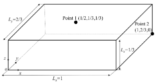
Figure 1: Physical model and coordinate definition. Two detection points 1 and 2 are set on the surface.

Hereafter, we shall address the heat conduction problem on the cuboid, denoted by domain $V$, as shown in Fig. 1. Its width $L_{x}$, depth $L_{y}$, and height $L_{z}$ are 1, 2/3 and 1/3, respectively. The surface of the cuboid is completely insulated. Two temperature detection points No. 1 and 2 are set at (1/2,1/3,1/3), and (1,2/3,0), respectively.

Initially the dimensional temperature $T$ in the cuboid is uniform at $T_{0}\textrm{ }(\theta=-1)$. At $t=0$, a uniform heat input $Q/(L_{y}L_{z})$ is given on the surface at $x=0$, introducing a temperature rise $\Delta T[=Q/(CV)]$ in the steady (equilibrium) state through the instantaneous total heat input $Q$ so that the steady temperature $T_{e}=T_{0}+\Delta T$. The rise provides the typical temperature difference to normalize the dimensional temperature $T$ as explained in the previous section.

In this section, a temperature-dependent thermal diffusivity of the form

$$a(\theta)=\left(\frac{c_{2}}{\theta+c_{2}}\right)^{c_{1}};\textrm{ power-law type}\textrm{ }(a_{1}=-c_{1}/c_{2}),$$

is considered, where coefficients $c_{i}\textrm{ }(i=1,2)$ are supposed to be positive number: $c_{1}$ is changed from 0 to 2.0, and $c_{2}$ is fixed at 3001 or 30001. The range of the parameters is typical for most pure metals (see Appendix B).

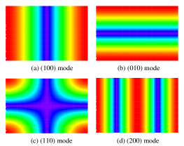
Figure 2: Top view of the first four slowest decaying modes ($z=1/3$): (a) (100) mode; (b) (010) mode; (c) (110) mode; (d) (200) mode. These figures show the absolute value of $\hat{v}_{lmn}$: the antinodal ($\left|\hat{v}\right|\fallingdotseq 3\sqrt{\psi(l)\psi(m)/2}$) and nodal ($\left|\hat{v}\right|\fallingdotseq 0$) regions are drawn in red and blue, respectively.

The heat conduction equation (16) was numerically solved by the finite volume method (FVM Smith (1965); Patankar (1980)). The diffusion term was discretized by the central difference scheme, and time integration was conducted by the first-order Euler explicit method. A used grid was $151\times 101\times 50$, and a time step was $3.66\times 10^{-6}$. The resolution can be numerically verified by comparison with the results on the double-resolution grid. The computations were performed by double precision.

The cuboid has the eigenfunction $\hat{v}_{lmn}$ and eigenvalue $\lambda_{lmn}$, specified by three non-negative integers $(lmn)$ as follows Strauss (1992); Ogi et al. (2016):

$$\lambda_{lmn} =\pi^{2}\left[\left(\frac{l}{L_{x}}\right)^{2}+\left(\frac{m}{L_{y}}\right)^{2}+\left(\frac{n}{L_{z}}\right)^{2}\right],$$

$$\hat{v}_{lmn}(\mathbf{x}) =\sqrt{\frac{\psi(l)\psi(m)\psi(n)}{L_{x}L_{y}L_{Z}}}\cos\left(\frac{l\pi x}{L_{x}}\right)\cos\left(\frac{m\pi y}{L_{y}}\right)\cos\left(\frac{n\pi z}{L_{z}}\right),$$

where $\psi(x)\equiv\min(2,x+1)$. Then the non-zero smallest four eigenvalues of the present model are

$$\lambda_{100}\fallingdotseq 9.86960,\textrm{ }\lambda_{010}\fallingdotseq 22.2066,\textrm{ }\lambda_{110}\fallingdotseq 32.0762,\textrm{ }\lambda_{200}\fallingdotseq 39.4784,$$

and, therefore, corresponding eigenfunctions are the four most slowest decaying modes. Their nodal and antinodal regions are illustrated in Fig. 2.

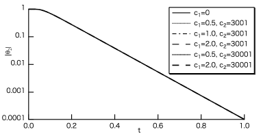
Figure 3: The absolute temperature variation at point 2 for the power-law-type thermal diffusivity. For any cases, the variations are almost identical.

Figure 3 shows the absolute temperature variation at point 2 for the case of power-law-type thermal diffusivity. The variation is independent of the coefficients $c_{1}$ and $c_{2}$, and its exponential decay rate 9.867 agrees well with that of (100) mode. Please note that the initial heat input exclusively excites ($n$00) ($n$: integer) modes and that (100) is the SDM among them. Herein, it is important that the decay rate of the SDM are not affected by the temperature-dependent thermal diffusivity.

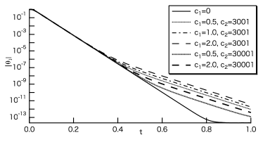
Figure 4: The absolute temperature variation at point 1 for the power-law-type thermal diffusivity. Thin and thick lines indicate the cases of $c_{2}=3001$ and 30001, respectively. Initially all lines are along the case of $c_{1}=0$, i.e. the case of constant diffusivity. Eventually, the lines separate and show the dependence on $c_{1}$ and $c_{2}$.

In contrast, as shown in Fig. 4, the temperature variation at point 1, bends at around $t=0.3\sim 0.4$ when $c_{1}$ is nonzero (not to be confused with a plateau at around $t=0.8$ for the case of a constant thermal diffusivity, $c_{1}=0$, caused by the round-off error around $10^{-13}$ ). The initial exponential decay ($t\lesssim 0.3$) does not depend on $c_{1}$ and $c_{2}$, and its decay rate 39.47 is in accord with that of (200) mode: the rSDM detected at point 1 is (200) mode because both excitation and detection are made on antinodal region of (200) mode. The (100) mode can not be observed on the point 1 because the point is the node of (100) mode. However, the later exponential decay depends on $c_{1}$ and $c_{2}$. For both of the two $c_{2}$ cases, the decay rate ranges from 19.27 $(c_{1}=0.5,\textrm{ }c_{2}=30001)$ to 19.89 $(c_{1}=0.5,\textrm{ }c_{2}=3001)$ and shows good agreement with $2\lambda_{100}(=19.74)$. This is the correction caused by the dependency, observed on the (200) mode. Please note, herein, that $\hat{v}_{100}^{2}$ corresponds to $\hat{v}_{200}$ except its constant component.

As $c_{2}$ is raised from 3001 to 30001, the bent point is delayed from $t$=0.3 to 0.4: the temperature-dependent property is weakened. Along the change, $|a_{1}|$ decreases approximately to 1/10. It implies that the parameter $a_{1}$ is significant for quantifying the dependent property (see Appendix B).

IV DISCUSSIONS AND CONCLUSIONS

The reduction of the Biot number $Bi$, i.e. sufficient insulation on the surface of specimen, holds the key to applicability of TMS. There are three reasons for that. First, we can not a priori know the distribution of heat transfer rate. We can define thermal modes for not the Neumann but the Robin boundary condition as explained in Sec. II. Such modes, however, highly depend on the fined distribution of heat transfer rate and, therefore, it is almost impossible for us in advance to know nodal and antinodal points for specifying a thermal mode. Second, we can not observe truly slowest decaying mode, i.e. uniform steady mode of zero decay rate. We have no choice but to regard a measured temperature decay rate as a non-zero decay rate of a target mode. If the uniform steady mode changes its eigenvalue to $S_{e}Bi/V$ by the minute heat transfer on the surface, described in Sec. III.1, the measured decay rate must be lower value by the contamination of the minute decay rate of the uniform SDM and, therefore, the thermal diffusivity is underestimated. Third, the decay rates of various modes are affected themselves by the heat transfer rate. The corrections were obtained by a perturbation analysis described in Sec. III.1.

In general, we can not regulate the corrections $\hat{\lambda}_{i}^{(n)}$ obtained in Sec. III.1 because they depend on given conditions such as the shape of specimen. All we can do is, therefore, reduce the Biot number $Bi$ so that $S_{e}Bi/V$ would be far smaller than the decay rate $\hat{\lambda}_{i}$ of a target mode. This is the de-facto insulated condition. Since the number is defined by $Bi=hL/k$, we can decrease the value by vacuuming or the reduction of typical specimen size $L$. Or it becomes small when a given specimen has high thermal conductivity. As explained in Sec. III.1, most measurement techniques request for the number to be sufficiently large. That is the reason why it is difficult to apply the methods to a small, like the order of 1mm Ogi et al. (2016), high-conductivity specimen. In contrast, TMS can rather conduct the measurement of such specimens with high-precision. It is certain that this is the major advantage of TMS method.

However, we should not restrict the application of TMS to the small-size, large thermal-diffusivity specimen. As described in Sec. III.3, the measurement of the decay rate of a specified mode has two advantages. First, the decay rate is measured after time passes sufficiently. In this final stage, the temperature variation within the specimen is very small, e.g. less than 0.03K (Ref. Ogi et al., 2016). The property allows us to identify the state in measurement with great accuracy as the temperature and pressure at thermal equilibrium without the introduction of such an effective temperature Parker et al. (1961). In addition, the decay rate of the SDM is identical with the rate at the equilibrium, not affected by the dependence of the thermal conductivity on temperature, as explained in Sec. III.3. In this sense, TMS truly overcomes the problem of the temperature dependency. This is also the great advantages of TMS. It is meaningful, therefore, to measure a low-diffusivity specimen in conjunction with some vacuuming techniques.

As explained in Sec. I, the Kapitza resistive film, i.e. the contact of a thin film with a specimen through the Kapitza resistance, is inevitable for most measurement techniques of thermal diffusivity. TMS has strength in this respect because the method is not so influenced by the Kapitza resistance in the sense that the first-order corrections to the decay rate caused by the film are independent of the Kapitza conductance, as explained in Sec. III.2. As long as the film thickness is sufficiently thin, therefore, there is no need for TMS to evaluate the conductance. This is the great advantage of TMS while most methods are required the evaluation to eliminate or to consider the first-order contributions Schmidt et al. (2009). The dimensionless film thickness $l$ is the ratio of a dimensional film thickness $l^{*}$ to a typical length $L$ of specimen. It is easy for us to reduce the thickness ratio less than $10^{-3}$ and, consequently, the errors caused by the films. We Ogi et al. (2016) actually achieved the ratio of $5.0\times 10^{-4}$ even for millimeter size specimens.

Herein, we should note that we can make thermal modes not affected by the resistive films. In Eq. (15), $\mathbf{x}^{T}\mathbf{Ny}$ and $\mathbf{x}^{T}\mathbf{Dy}$ present the integrated product of functions $x,y$ and of their gradients on an attached-film surface $S_{e}$, respectively. In TMS, such a surface is positioned at the excitation or detection point, selected so that it is at an antinode of a target mode, say $i$th mode, and also at a node of a mode, say $k$th mode, to be eliminated. The mode-selection principle does remove the first-order correction $w_{i,k}^{(1)}$ (Eq. (15b)), significant for TMS.

This is also the case for the effects of heat transfer rate. If we can insulate the surface of the specimen except the excitation and detection points, similar discussion deduces that the first-order correction $w_{i,k}^{(1)}$ (Eq. (10b)) of thermal mode vanishes. The condition is naturally fulfilled when we are to insulate the surface of specimen as much as possible: such insulation is impossible near the excitation and detection points. In both cases, therefore, thermal modes are assumed to be kept unchanged for the cases of small heat transfer rate and thin Kapitza resistive film. It is significant for the mode-selection principle.

Appendix A HEAT CONDUCTION EQUATION ON A SPECIMEN WITH KAPITZA RESISTIVE FILMS

On the platform of the ODEs described in Sec. III.1, we shall incorporate the Kapitza resistive films as a boundary condition within a portion of the specimen surface, and derive a closed heat conduction equation for an arbitrary-shape specimen with arbitrary-shape resistive films.

Now we begin with a formulation of a film (domain $V^{\prime}$) attached to a portion $Se$ on a specimen. Application of the form (6) to the film yields the evolution equation for film temperature $\bm{\uptheta^{\prime}}$ as follows:

$$\mathbf{M^{\prime}}\frac{d\bm{\uptheta^{\prime}}}{dt}=-\mathbf{\Gamma^{\prime}}\bm{\uptheta^{\prime}}+\mathbf{c^{\prime}},$$ (20a)

where

$$\mathbf{M^{\prime}}=\{M^{\prime}_{\alpha\beta}:\textrm{ }\mathit{M^{\prime}_{\alpha\beta}=C^{\prime}\int_{V^{\prime}}\varphi_{\alpha}\varphi_{\beta}dV},\textrm{ }1\leq\alpha,\beta\leq N\},$$ (20b)

$$\mathbf{\Gamma^{\prime}}=\{\varGamma^{\prime}_{\alpha\beta}:\textrm{ }\mathit{\Gamma^{\prime}_{\alpha\beta}=k^{\prime}\int_{V^{\prime}}\sum_{j}\frac{\partial\varphi_{\alpha}}{\partial x_{j}}\frac{\partial\varphi_{\beta}}{\partial x_{j}}dV},\textrm{ }1\leq\alpha,\beta\leq N\},$$ (20c)

$$\mathbf{c^{\prime}}=\{c^{\prime}_{\alpha}:\textrm{ }\mathit{c^{\prime}_{\alpha}=\int_{S_{e}}f_{n}\varphi_{\alpha}dS},\textrm{ }1\leq\alpha\leq N\},$$ (20d)

and the variable $C^{\prime}$ is the ratio of volumetric specific heat of the film to that of the specimen. The heat conductivity ratio $k^{\prime}$ is similarly defined. In this formulation the flux $f_{n}$ is defined as the heat flux in the direction of inward pointing normal vector on the film-specimen boundary $Se$: by use of the thermal contact condition, it turns out to be the outward normal heat flux from the specimen.

Expanding the flux $f_{n}$ by the basis functions $\varphi_{\beta}$ as follows

$$\left.f_{n}(\mathbf{x},t)\right|_{\mathbf{x}\in S_{e}}=\left.\sum_{\beta}f{}_{\beta}(t)\varphi_{\beta}(\mathbf{x})\right|_{\mathbf{x}\in S_{e}},$$

and substituting into Eq. (20d) we obtain

$$\mathbf{c^{\prime}}=\mathbf{Nf},$$ (21a)

where

$$\mathbf{f}\equiv(f_{1},\cdots,f_{N}),$$ (21b)

$$\mathbf{N}=\{N{}_{\alpha\beta}:\textrm{ }\mathit{N_{\alpha\beta}=\int_{Se}\varphi_{\alpha}\varphi_{\beta}dS},\textrm{ }1\leq\alpha,\beta\leq N\}.$$ (21c)

In order to obtain a solution to hold the quiescent initial condition, the Laplace transform of Eq. (20a) with a complex variable $s$ is utilized to find

$$\bar{\mathbf{f}}=\mathbf{\Xi^{\prime}}\bm{\bar{\uptheta}^{\prime}},\textrm{ }\mathbf{\Xi^{\prime}}\equiv\mathbf{N}^{-1}(s\mathbf{M^{\prime}}+\mathbf{\Gamma^{\prime}}),$$ (22)

where $\bar{\mathbf{f}}$ and $\bm{\bar{\uptheta}^{\prime}}$ are the Laplace transforms of $\mathbf{f}$ and $\bm{\uptheta^{\prime}}$, respectively. Herein, as defined by Eq. (21c), $\mathbf{N}$ is positive-definite and, therefore, its inverse can be defined.

The Kapitza conductance $\alpha$ at the film-specimen interface makes a surface temperature gap on both sides. When $\bm{\bar{\uptheta}}$ denote the Laplace transform of the temperature $\bm{\uptheta}$ on the specimen surface $Se$, a dimensionless thermal contact condition leads to $\bar{\mathbf{f}}=l_{K}^{-1}(\bm{\bar{\uptheta}}-\bm{\bar{\uptheta}^{\prime}})$, where $l_{K}\equiv(k/\alpha)/L$ is the ratio of the so-called Kapitza length $k/\alpha$ to the typical length. Substituting the relation into Eq. (22) yields

$$\bar{\mathbf{f}} =(\mathbf{I}+l_{K}\mathbf{\Xi^{\prime}})^{-1}\mathbf{\Xi^{\prime}}\bm{\bar{\uptheta}}$$

$$=(\mathbf{I}-l_{K}\mathbf{\Xi^{\prime}}+l_{K}^{2}\mathbf{\Xi^{\prime}}^{2}-l_{K}^{3}\mathbf{\Xi^{\prime}}^{3}+\cdots)\mathbf{\Xi^{\prime}}\bm{\bar{\uptheta}}$$

$$\equiv\mathbf{A}^{\prime}\bm{\bar{\uptheta}}$$ (23a)

$$\equiv(\mathbf{A}^{\prime}_{0}-s\mathbf{A}^{\prime}_{1}+\cdots+(-s)^{n}\mathbf{A}^{\prime}_{n}+\cdots)\bm{\bar{\uptheta}}.$$ (23b)

On the other hand, the evolution equation (6a) of specimen temperature is modified to be

$$\mathbf{M}\frac{d\bm{\uptheta}}{dt}=-\mathbf{\Gamma}\bm{\uptheta}-\mathbf{Nf}.$$ (24)

Substituting of the inverse Laplace transform of Eq. (23b) into the above equation, we eventually obtain a closed governing equation for specimen temperature as follows:

$$\mathbf{M}\dot{\bm{\uptheta}}+\mathbf{\Gamma}\bm{\uptheta}+\mathbf{N}(\mathbf{A}^{\prime}_{0}\bm{\uptheta}-\mathbf{A}^{\prime}_{1}\dot{\bm{\uptheta}}+\mathbf{A}^{\prime}_{2}\ddot{\bm{\uptheta}}+\cdots+(-1)^{n}\mathbf{A}^{\prime}_{n}\bm{\uptheta}^{(n)}+\cdots)=0.$$ (25)

If we have more than one ($R$) resistive films, the third term of the left-hand side of the equation should be replaced by

$$\sum_{i=1}^{R}\mathbf{N}_{i}(\mathbf{A}_{0}^{(i)^{\prime}}\bm{\uptheta}-\mathbf{A}_{1}^{(i)^{\prime}}\dot{\bm{\uptheta}}+\mathbf{A}_{2}^{(i)^{\prime}}\ddot{\bm{\uptheta}}+\cdots).$$

Appendix B INDICATOR OF DEPENDENCY OF THERMAL DIFFUSIVITY ON TEMPERATURE

In order to elucidate the importance of parameter $a_{1}$ as the indicator of temperature-dependent properties, in this section, two types of thermal diffusivity are tested:

$$a(\theta)=\begin{cases}e^{-c_{3}\theta}&;\textrm{ exponential type }(a_{1}=-c_{3}),\\ \frac{1}{\left(1+\theta^{2}\right)^{c_{4}}}&;\textrm{ modified power-law type }(a_{1}=0),\end{cases}$$

where coefficients $c_{i}\textrm{ }(i=3,4)$ are also supposed to be positive number.

The coefficient $a_{1}$ for each case is obtained from Eq. (17a). By use of dimensional thermal diffusivity $a^{*}(T)$, it can be rewritten as

$$a_{1}=\left.\frac{1}{a}\frac{\partial a}{\partial\theta}\right|_{\theta=0}=\frac{\Delta T}{a^{*}(Te)}\left.\frac{\partial a^{*}}{\partial T}\right|_{T=T_{e}},$$ (26)

and, therefore, it can be regarded as the normalized exponential increase rate of thermal diffusivity at the steady state.

Most pure metals Gray (1972); jsm (2009) have the dimensional coefficient $c_{3}^{*}$ of the order of $10^{-4}\sim 10^{-3}$, and have the coefficient $c_{1}<1$. If the temperature rise $\Delta T$ is of the order of $0.01\sim 0.1$K (see, for example, Ref. Ogi et al., 2016), the coefficient $c_{3}(=c_{3}^{*}\Delta T)$ is estimated to be $10^{-6}\sim 10^{-4}$. On the other hand, the coefficient $c_{2}\equiv T_{e}/\Delta T$ is of the order of $10^{3}\sim 10^{4}$ when $T_{e}$ is near a room temperature and $\Delta T$ is $0.01\sim 0.1$K. In this study $c_{2}$ is fixed at 3001 or 30001, and $c_{1}$ is changed from 0 to 2.0. It follows that the order of $c_{3}(\sim c_{1}/c_{2})$ is less than that of $10^{-4}\sim 10^{-3}$. $c_{4}$ is changed from 0 to 1.0 because double the value corresponds to $c_{1}$.

The physical model and the discretization of the heat conduction equation are the same as those explained in Sec. III.3.2. Most computations (except one case mentioned below) were performed by double precision.

First of all, the computations by the exponential-type thermal diffusivity, corresponding to Figs. 3 and 4, are performed under the same initial condition. With the coefficient $c_{3}$ held fixed at $c_{1}/c_{2}$, i.e. with the corresponding two $a_{1}$’s being identical, we can confirm that temperature variations for the exponential type agree up to the first five digit numbers with the variations of the power-law-type diffusivity, and they can not be distinguished on Figs. 3 and 4. These results indicate that the coefficient $a_{1}$ is important for the temperature-dependent properties.

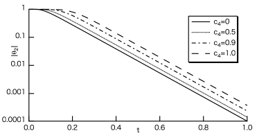
Figure 5: The absolute temperature variation at point 2 for the modified power-law-type thermal diffusivity. Unlike Fig. 3, the initial variations are strongly affected by $C_{4}$. In the final stage, however, every line decays with the same rate.

When we choose the modified power-law-type diffusivity, temperature variations become simple. In this type of dependency $a_{1}$ is fixed at zero. Figure 5 shows the temperature variation at point 2. Since the diffusivity is far smaller than that of power-law type for $\theta>10$, the temperature initially remains constant when $c_{4}$ is large. But it eventually shows exponential decay whose decay rate ranges from 9.864 ($c_{4}$=0.9) to 9.867 ($c_{4}$=0), in agreement with that of (100) mode.

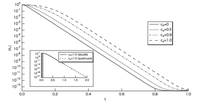
Figure 6: The absolute temperature variation at point 1 for the modified power-law-type thermal diffusivity. Unlike Fig. 4, every line decays with a single rate, saturating around the order of its round-off error, $10^{-13}$. On the other hand, the inset shows the result of quadruple-precision computation. The line decays to reach around the order of its round-off error, $10^{-31}$. Even with this accurate computation, we can not find the effects of $a_{2}$ or higher-order corrections.

As shown in Fig. 6, the variation at point 1 does not show the bent: its exponential decay rate ranges from 39.32 ($c_{4}$=0.9) to 39.47 ($c_{4}$=0), almost identical with that of (200) mode. The effects of higher-order corrections or $a_{2}$ can appear in the final, minute temperature variation in the vicinity of the thermal equilibrium. In this study, therefore, a computation by quadruple precision is performed and the result is shown in the inset of Fig. 6. The temperature shows a single exponential decay eventually to reach the order of round-off error $10^{-31}$, lower than the limit of temperature measurement. There is no evidence that higher-order corrections appear. The results clarified that the normalized exponential increasing rate $a_{1}$ of thermal diffusivity can be regarded as the indicator to quantify the effects of temperature-dependent thermal diffusivity.

From the expression (26) of $a_{1}$, we might expect that it is reducible by diminishing the (typical) temperature rise $\Delta T$ caused by the heat input in measurement. However, it depends on the property of a specimen. From the discussion in Fig. 4, we confirmed that the bent point $t_{b}$, i.e. the time when the effects of temperature dependence appear, is delayed from 0.3 to 0.4. We can extrapolate the result to estimate that $a_{1}$ should be less than $1.0\times 10^{-8}$ to hold the condition that $t_{b}=1$ for the accurate measurement of the decay rate. For most pure metals the dimensional exponential increase rates of diffusivity are typically the order of $10^{-4}\sim 10^{-3}$ (1/K), it follows that $\Delta T$ must be less than $10^{-5}\sim 10^{-4}$ (K). Thereby it is difficult for us accurately to detect temperature evolution.

Thus, we need the plan to avoid such a situation. The temperature change shown in Fig. 4 is caused by the selection of not the SDM [(100) mode] but (200) mode (rSDM) as the target among excited modes. If the point 2 were chosen, we could have measured the decay rate $\lambda_{SDM}$ of the SDM as shown in Fig. 3. It follows that the detection mode must be in accord with the SDM among the excited modes except the case that we measure in a positive manner the decay rate of $2\lambda_{SDM}$ for the case of temperature-dependent thermal diffusivity.

References

- Ångström (1861) A. J. Ångström, Ann. Phys. Chem. 114, 513 (1861).
- Ångström (1863) A. J. Ångström, Phil. Mag. 25, 130 (1863).
- Schleiermacher (1888) A. Schleiermacher, Ann. Phys. Chem. 34, 623 (1888).
- Andersson and Bäckström (1973) P. Andersson and G. Bäckström, J. Appl. Phys. 44, 2601 (1973).
- Kraemer and Chen (2014) D. Kraemer and G. Chen, Rev. Sci. Instrum. 85, 025108 (2014).
- King (1915) R. W. King, Phys. Rev. 6, 437 (1915).
- Sidles and Danielson (1954) P. H. Sidles and G. C. Danielson, J. Appl. Phys. 25, 58 (1954).
- Ingersoll and Koepp (1924) L. R. Ingersoll and O. A. Koepp, Phys. Rev. 24, 92 (1924).
- Frazier (1932) R. H. Frazier, Phys. Rev. 39, 515 (1932).
- Zhang et al. (2006) X. Zhang, H. Gu, and M. Fujii, J. Appl. Phys. 100, 044325 (2006).
- Cahill and Pohl (1987) D. G. Cahill and R. O. Pohl, Phys. Rev. B 35, 4067 (1987).
- Wang et al. (2007) Z. L. Wang, D. W. Tang, S. Liu, X. H. Zheng, and N. Araki, Int. J. Thermophysics 28, 1255 (2007).
- Schmidt et al. (2009) A. J. Schmidt, R. Cheaito, and M. Chiesa, Rev. Sci. Instrum. 80, 094901 (2009).
- Adams et al. (1976) M. J. Adams, A. A. King, and G. F. Kirkbright, Analyst 101, 73 (1976).
- Astrath et al. (2012) F. B. G. Astrath, N. G. C. Astrath, M. L. Baesso, A. C. Bento, J. C. S. Moraes, and A. D. Santos, J. Appl. Phys. 111, 014701 (2012).
- Parker et al. (1961) W. Parker, R. Jenkins, C. Butler, and G. Abbott, J. Appl. Phys. 32, 1679 (1961).
- Baba and Ono (2001) T. Baba and A. Ono, Meas. Sci. Technol. 12, 2046 (2001).
- Paddock and Eesley (1986) C. A. Paddock and G. L. Eesley, J. Appl. Phys. 60, 285 (1986).
- Capinski and Maris (1996) W. S. Capinski and H. J. Maris, Rev. Sci. Instrum. 67, 2720 (1996).
- Alwi et al. (2013) H. A. Alwi, Y. Kim, R. Awang, S. Rahman, and S. Krishnaswamy, Int. J. Heat Mass Transfer 63, 199 (2013).
- Hatta et al. (1985) I. Hatta, Y. Sasuga, R. Kato, and A. Maesono, Rev. Sci. Instrum. 56, 1643 (1985).
- Hashimoto et al. (1990) T. Hashimoto, Y. Matsui, A. Hagiwara, and A. Miyamoto, Thermochimica Acta 163, 317 (1990).
- Cifuentes et al. (2016) A. Cifuentes, S. Alvarado, H. Cabrera, A. Calderón, and E. Marín, J. Appl. Phys. 119, 164902 (2016).
- Wang et al. (2016) T. Wang, S. Xu, D. H. Hurley, Y. Yue, and X. Wang, Opt. Lett. 41, 80 (2016).
- Ogi et al. (2016) H. Ogi, T. Ishihara, H. Ishida, A. Nagakubo, N. Nakamura, and M. Hirao, Phys. Rev. Lett. 117, 195901 (2016).
- Migliori et al. (1993) A. Migliori, J. Sarrao, W. M. Visscher, T. Bell, M. Lei, Z. Fisk, and R. Leisure, Physica B 183, 1 (1993).
- Maynard (1996) J. Maynard, Phys. Today 49, 26 (1996).
- Ogi et al. (1999) H. Ogi, H. Ledbetter, S. Kim, and M. Hirao, J. Acoust. Soc. Am. 106, 660 (1999).
- Ogi et al. (2002) H. Ogi, K. Sato, T. Asada, and M. Hirao, J. Acoust. Soc. Am. 112, 2553 (2002).
- Strauss (1992) W. A. Strauss, Partial Differential Equations: An Introduction (John Wiley & Sons, Inc., 1992).
- Smith (1965) G. D. Smith, Numerical Solution of Partial Differential Equations (Oxford University Press, New York, 1965).
- Patankar (1980) S. V. Patankar, Numerical Heat Transfer and Fluid Flow (Taylor & Francis, London, 1980).
- Gray (1972) D. E. Gray, ed., American institute of physics handbook, 3rd ed. (McGraw-Hill, New York, 1972).
- jsm (2009) JSME Data Book: Heat Transfer, 5th ed. (Maruzen Co. Ltd., Tokyo, 2009) (in Japanese).