Core Emergence in a Massive Infrared Dark Cloud:
A Comparison Between Mid-IR Extinction and 1.3 mm Emission

Abstract

Stars are born from dense cores in molecular clouds. Observationally, it is crucial to capture the formation of cores in order to understand the necessary conditions and rate of the star formation process. The Atacama Large Mm/sub-mm Array (ALMA) is extremely powerful for identifying dense gas structures, including cores, at mm wavelengths via their dust continuum emission. Here we use ALMA to carry out a survey of dense gas and cores in the central region of the massive ($\sim 10^{5}\>M_{\odot}$) Infrared Dark Cloud (IRDC) G28.37+0.07. The observation consists of a mosaic of 86 pointings of the 12m-array and produces an unprecedented view of the densest structures of this IRDC. In this first paper about this data set, we focus on a comparison between the 1.3 mm continuum emission and a mid-infrared (MIR) extinction map of the IRDC. This allows estimation of the “dense gas” detection probability function (DPF), i.e., as a function of the local mass surface density, $\Sigma$, for various choices of thresholds of mm continuum emission to define “dense gas”. We then estimate the dense gas mass fraction, $f_{\rm dg}$, in the central region of the IRDC and, via extrapolation with the DPF and the known $\Sigma$ probability distribution function, to the larger-scale surrounding regions, finding values of about 5% to 15% for the fiducial choice of threshold. We argue that this observed dense gas is a good tracer of the protostellar core population and, in this context, estimate a star formation efficiency per free-fall time in the central IRDC region of $\epsilon_{\rm ff}\sim$10%, with approximately a factor of two systematic uncertainties.

1. Introduction

Dense cores, as the birthplace of stars, are the focus of intense theoretical and observational study, in particular for understanding the initial conditions and efficiency of star formation (see, e.g., Bergin & Tafalla, 2007; Tan et al., 2014; Offner et al., 2014). One theory of core formation is that of gravito-turbulent fragmentation where dense, gravitationally unstable cores are created in density perturbations arising from compressions in supersonically turbulent molecular gas (e.g., Padoan & Nordlund, 2002; Krumholz & McKee, 2005; Hennebelle & Chabrier, 2008; Chabrier et al., 2014). In the theory of Krumholz & McKee (2005) (see also Padoan & Nordlund, 2011) the rate of star formation is linked to the Mach number and virial parameter (i.e., degree of gravitational boundedness) of the cloud, although it should be remembered that most of the numerical simulation results that underpin these models are of periodic box turbulence (rather than of global cloud structures) and have relatively weak magnetic fields (i.e., are globally magnetically supercritical) (see Tan, 2016). Models of core formation mediated by magnetic fields, e.g., via ambipolar diffusion (Kunz & Mouschovias, 2009; Christie et al., 2017), have also been proposed.

Giant molecular clouds (GMCs) in the Milky Way are known to have a low star formation efficiency (SFE) (Zuckerman & Evans, 1974; Kennicutt & Evans, 2012), where this quantity is most naturally evaluated as the fraction of mass that forms stars in one local free-fall time of the gas, i.e., $\epsilon_{\rm ff}$, which is seen to have a value of about 0.02. Krumholz & Tan (2007) extended the analysis methods of Zuckerman & Evans (1974) to denser gas structures, such as Infrared Dark Clouds (IRDCs) and embedded clusters, finding similar values of $\epsilon_{\rm ff}$. Murray (2011) and Lee et al. (2016) have pointed out there is a large dispersion in $\epsilon_{\rm ff}$ in Galactic GMCs, but the average value in the population is still low and consistent with prior estimates. Theoretical models of star formation rates (SFRs) regulated by turbulence (e.g., Krumholz & McKee, 2005; Hennebelle & Chabrier, 2011; Krumholz et al., 2012) are one way to explain the low averaged observed values of $\epsilon_{\rm ff}$. However, Lee et al. (2016) have noted that the high dispersion in $\epsilon_{\rm ff}$ is not accounted for in these models. This may imply a role for more stochastic processes, such as triggering by collisions of magnetically supported GMCs inducing bursts of star formation activity (Scoville et al., 1986; Tan, 2000; Wu et al., 2015, 2017).

In order to observationally capture the formation of cores and have a sneak peek of the signature of low SFE, we can compare features that are specifically sensitive to the core formation with features representing the host cloud. Dust continuum emission at mm wavelength is sensitive to star-forming cores and often used as a core tracer (e.g., Bergin & Tafalla, 2007; Sanhueza et al., 2017). If observed with interferometers like ALMA, mm continuum emission can potentially pinpoint dense, star-forming cores embedded in a molecular cloud because the extended emission is resolved out by interferometers. Moreover, continuum emission does not depend on chemical abundance variations (such as chemical depletion) which can affect molecular-line-defined cores. The host cloud, and its density structure, can be traced by far-infrared dust emission (André et al., 2014) or dust extinction (Lombardi, 2009; Butler & Tan, 2009). The latter has been used to construct $\Sigma$ probability distribution functions ($\Sigma$-PDF, e.g., Kainulainen et al., 2009; Butler et al., 2014; Stutz & Kainulainen, 2015; Lim et al., 2016). Such distributions appear to have a log-normal component, perhaps arising from turbulence, together with a high-$\Sigma$ power law tail, perhaps due to self-gravity. However, observationally it is challenging to accurately measure the $\Sigma$-PDF (e.g., Alves et al., 2017; Chen et al., 2017). Numerical simulations of molecular clouds also aim to reproduce the $\Sigma$-PDF and understand its dependence on the included physics (see, e.g., Collins et al., 2011; Federrath & Klessen, 2013; Myers, 2015).

In this paper, we study the relationship between mm continuum emitting dense gas structures and the local mass surface density of their hosting cloud to better understand the conditions of core formation. Our target cloud is IRDC G28.37+0.07 (also referred to as IRDC C) from the sample of Butler & Tan (2009, 2012, hereafter BT09, BT12) at an estimated kinematic distance of 5 kpc. Specifically, we compare the mid-infrared (MIR) extinction map of the IRDC (Butler et al., 2014, hereafter BTK14) with a newly acquired 1.3 mm continuum image, observed with ALMA.

2. Data

2.1. ALMA Observations

The observations were carried out between 24-Jun-2016 and 30-Jun-2016 (UTC) (ALMA Cycle 3), under the project 2015.1.00183.S (PI: Kong). Forty-six 12-m antennas were used during the observation in C40-4 configuration. A custom mosaic with 86 pointings was used to cover the majority of the central dark regions of IRDC G28.37+0.07. The observations were in band 6 ($\sim$ 231 GHz). A baseband of 1.8 GHz was used for the 1.3 mm continuum observation (the effective bandwidth for continuum imaging is $\sim 1.4\>$GHz due to the exclusion of the ¹²CO(2-1) molecular line). Three other basebands were set for molecular line observations. In this paper, we focus on the continuum data; we defer the analysis of the molecular line data to a future paper.

The observations consist of 6 scheduling blocks, each having roughly 50 minutes on-source integration time. J1751+0939 and J1924-2914 were used as bandpass calibrators. J1751+0939, J1924-2914, and Titan were used as flux calibrators. J1851+0035 was used as the phase calibrator. The typical system temperature was 80 K. The mosaic image was cleaned using the standard clean task in CASA. Briggs weighting with a robust number of 0.5 was applied. No self-calibration was done. In order to perform a pixel-by-pixel comparison with the MIREX image (see following section), we applied an outer uv-taper to match the ALMA synthesized beam to the MIREX beam (2″). A pixel scale of 0.4″ was adopted in the clean task. Then we re-binned the images to have 1.2″ pixels to match the MIREX pixel scale. The resulting sensitivity at map center is $\sigma_{\rm center}=$ 0.2 mJy per 2″ beam. The maximum recoverable scale of the ALMA continuum image is $\sim$20″ (corresponding to the shortest baseline of 10 k$\lambda$ with $\lambda$ being 1.3 mm).

2.2. The MIREX image

The MIR extinction (MIREX) map of IRDC G28.37+0.07 was first developed by BT09 and BT12 using Spitzer 8 $\rm\mu m$ GLIMPSE imaging data (Churchwell et al., 2009). It was merged with a lower resolution NIR extinction map by Kainulainen & Tan (2013), which improves accuracy at lower values of $\Sigma$. Finally, the map was refined by Butler et al. (2014) by using an analysis of deeper archival Spitzer-IRAC imaging, which enables the highest dynamic range of $\Sigma$ to be probed. In general, the method of MIREX mapping involves estimating the intensity of the diffuse background emission, i.e., from the diffuse Galactic ISM, via interpolation from surrounding regions, and estimating, empirically, the level of the foreground emission. Then, given an estimate of the dust opacity at 8 $\rm\mu m$ (averaged over the Spitzer IRAC Band 4) and a dust to gas mass ratio, the total mass surface density can be calculated by solving the simple 1D radiative transfer equation, given the observed intensities emerging from the cloud. The spatial resolution achieved in the map is 2″with a pixel scale of 1.2″, set by the resolution of the Spitzer-IRAC data.

There are several effects that lead to systematic errors in the MIREX maps. One problem is that in regions containing local bright MIR source, the extinction is contaminated by the source. Another problem is that in some regions the IRDCs become very optically thick, so only a lower limit on $\Sigma$ can be estimated. These regions are referred to as being “saturated” in the MIREX map (their presence allows the measurement of the diffuse foreground emission, assumed to be spatially constant). Local fluctuations in the background will lead to errors, since it is modeled as a smoothly varying source. Zero point offsets of up to $\sim 0.1\>{\rm g\>cm}^{-2}$ are present, which are partially corrected for by calibration with NIR extinction maps (Kainulainen & Tan, 2013). Still, the zero point uncertainty is present at a level estimated to be $\sim 0.02\>{\rm g\>cm}^{-2}$ (i.e., $A_{V}\sim 4$ mag or so).

3. Results

3.1. Comparison between 1.3 mm Dust Continuum Emission and MIR Extinction

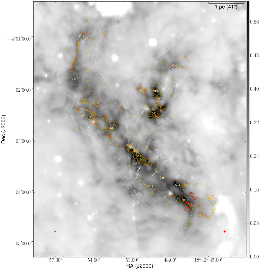
Figure 1.— Greyscale: MIREX mass surface density map from BTK14 (scale in g cm^-2). The angular resolution of the map is shown as the gray filled circle at lower-left. “C1, C2, C3…” label extinction peaks from BTK14. The white arrows point to possible embedded protostars that show as local enhancements in the $\rm 8\>\mu m$ image, which produce local “holes” in the MIREX map. Contours: ALMA 1.3 mm continuum mosaic. The contours range from SNR = 2, 3, 5, 10, 20, 40, 60, … with the rms noise at map center $\sigma_{\rm center}\sim 0.2\rm mJy\>beam^{-1}$. The two red contours highlight SNR = 3 and 10. The synthesized beam is shown as the red filled ellipse at lower-right. The two white enclosing contours show primary-beam responses of 0.3 (outer) and 0.5 (inner).

Figure 1 shows the comparison between the cloud mass surface density from the MIREX map and the 1.3 mm dust continuum emission observed by ALMA. In general, the MIREX image shows mainly $\Sigma\gtrsim 0.2\>$g cm^-2 pixels in the ALMA-mosaicked region. They correspond to relatively dark regions in the original Spitzer IRAC 8$\rm\mu m$ image. The MIREX map reveals features via dust absorption (depending on total $\Sigma$), while the ALMA image shows dust emission (depending on total $\Sigma$ and dust temperature). Another difference arises due to ALMA filtering out low spatial frequency (larger-scale) structures. In our case, the recoverable physical scales range from 10,000 AU (0.05 pc, 2″) (after uv-tapering) to approximately 100,000 AU (0.48 pc, 20″). We note that the Jeans length

$$\lambda_{J}=0.10\left(\frac{T}{15\>\rm K}\right)^{1/2}\left(\frac{n_{\rm H}}{10^{5}\>\rm cm^{-3}}\right)^{-1/2}\>\rm pc$$ (1)

is in the range of recovered scales, given typical conditions of ambient gas in the IRDC. Consequently, while the extinction map tracks the total column density, the ALMA continuum image pinpoints compact, dense and warmer structures, i.e., expected to be protostellar cores. Thus, through comparison with the extinction map, the ALMA image shows us where such dense, likely star-forming, structures emerge from the cloud.

We now give a brief overview of several of the regions seen in the map. Dense “cores/clumps” C1 to C16 were identified in the MIREX map by BT12 and BTK14. The continuum cores in the south-west C1 region were studied by Tan et al. (2013, 2016); Kong et al. (2017). C1-Sa and C1-Sb have been identified as protostellar cores and C1a and C1b as candidate protostellar cores. A massive pre-stellar core candidate, C1-S, identified by $\rm N_{2}D^{+}(3-2)$ emission by Tan et al. (2013), sits between C1-Sa and C1-Sb, but has relatively faint 1.3 mm continuum emission. C1 is the location of the C1-N core, which is another massive pre-stellar core candidate identified by its $\rm N_{2}D^{+}(3-2)$ emission. We note that most of the protostellar cores (including the relatively low-mass $\sim 2\>M_{\odot}$ C1-Sb core) and some massive pre-stellar cores are well-detected in the ALMA continuum image.

Moving to the NE, several other sources are seen in the region, including the C14, C15 and C16 core/clumps. Next we come to the C2 region, which corresponds to the “P1 clump” studied by Zhang et al. (2009, 2015). They identified a linear chain of five main continuum structures, with a hint of a sixth core/clump at the SW end. Here we confirm the detection of this sixth, weaker continuum structure. Like the other cores, it also corresponds to a high-$\Sigma$ peak in the MIREX map. With the higher resolution ($\sim 0.7\arcsec$) observations of Zhang et al. (2015) a few tens of cores were identified in the C2 region down to sub-solar masses, with many of these seen to be protostellar by the presence of bipolar CO outflows.

North-west of C2 is a region containing C4, C10 and C13, with most of the mass concentrated near C4 and C13. Several distinct mm continuum peaks are visible in this region. Continuing north-east from C2 is the sequence of MIR dark core/clumps C5 and C6, which contain a cluster of mm emission cores, then the sparser C11 and C12. Between C11 and C12 there is a narrow filament seen in mm continuum emission, which closely follows the morphology seen in the MIREX map. This filament shows signs of fragmenting into several cores (including C12), but may be at an earlier stage of evolution compared to the more fragmented regions described above, such as C5/C6, C4/C13 and perhaps C2.

Globally, Figure 1 shows that the 1.3 mm continuum structures follow the extinction features quite well, i.e., they tend to be found in high-$\Sigma$ regions of the MIREX map. For example, in the region around C4, the cloud shows very good agreement between the continuum emission and high-$\Sigma$ pixels. On the other hand, MIREX high-$\Sigma$ regions do not always show mm continuum emission. This is illustrated in the region around C11, where it shows few robust 1.3 mm continuum detections. Being in a high-$\Sigma$ region is a necessary, but not sufficient, condition for the presence of strong mm continuum cores.

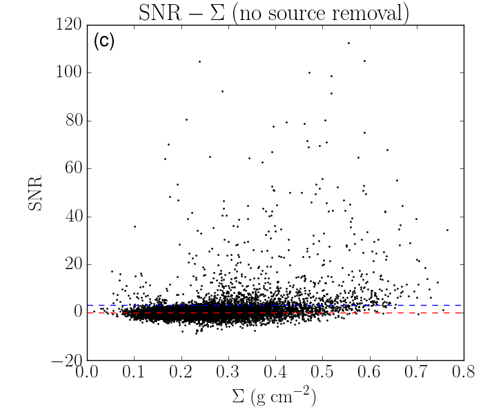
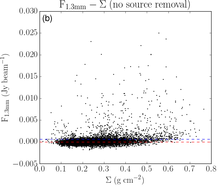
Figure 2.— (a) Pixel-by-pixel comparison between SNR and $\Sigma$. The red dashed line shows the zero point of the continuum image. The blue dashed line shows the SNR = 3 noise level. The map boundary is defined where the primary-beam response is 0.5. (b) Pixel-by-pixel comparison between $F_{\rm 1.3mm}$ and $\Sigma$. The map boundary is defined where the primary-beam response is 0.5 (see Figure 1). The noise at the map center $\sigma_{\rm center}$ (indicated by the blue dashed line) is a factor of 2 smaller than at the edge. (c) Same as (a) but removing the embedded sources. See §3.2. (d) Same as (b) but removing the embedded sources. See §3.2.

In order to reveal more quantitatively the large-scale mass surface density conditions needed for the formation of 1.3 mm continuum emitting structures, we make a pixel-by-pixel comparison between the ALMA image and the MIREX image (Figure 2). We show two different types of comparison. In panel (a), we compare signal-to-noise ratio (SNR) and $\Sigma$. In panel (b), we compare the 1.3 mm continuum flux density $F_{\rm 1.3mm}$ with $\Sigma$. The continuum image is primary-beam corrected, so the map boundary regions have higher noise levels. Both comparisons are restricted to regions where the ALMA primary-beam response $\geq$0.5. In both panels, we show the 3$\sigma_{\rm center}$ noise level with a blue dashed horizontal line. The zero point is shown as the red dashed horizontal line. A $3\sigma_{\rm center}$ noise corresponds to a continuum-derived mass surface density $\Sigma_{\rm mm}$ = 0.044 g cm^-2 (using equation 1 in Kong et al., 2017), assuming a dust temperature of 20 K, $\kappa_{\nu}=5.95\times 10^{-3}\>{\rm cm^{2}\>g^{-1}}$ (the moderately coagulated thin ice mantle model of Ossenkopf & Henning, 1994), i.e., with a dust-to-gas mass ratio of 1:141 (Draine, 2011). For a mean particle mass of 2.33$m_{\rm H}$ (i.e., $n_{\rm He}=0.1n_{\rm H}$), this corresponds to a total column density $N_{\rm H}=1.9\times 10^{22}\>$cm^-2, i.e, a visual extinction of $A_{V}=9.4\>$mag (assuming an extinction to column density relation $A_{V}=(N_{\rm H}/2.0\times 10^{21}\>{\rm cm}^{-2})\>$mag). We note that our restriction of analysis to the region where the primary-beam correction factor is $<2$ means that uncertainties associated with this correction are minimized to this level or smaller.

At first glance, the plots show no clear correlation between the mm continuum flux and MIREX $\Sigma$. A similar situation was found by Johnstone et al. (2004) comparing 0.85 mm continuum emission (observed with JCMT) and near infrared extinction (derived from 2MASS data). However, Figure 2, shows a hint of detection deficit of mm continuum emission at $\Sigma\lesssim 0.15\rm g~{}cm^{-2}$, although there are still a modest number of relatively high SNR and flux density values in this regime. However, one important systematic error associated with the MIREX map is the presence of MIR-bright sources, which lead to an underestimation of $\Sigma$ at these locations. We carry out a visual identification of potential MIR sources in the Spitzer IRAC $8\>{\rm\mu m}$ image and mark their locations in Figure 1. We then remove these pixels from the analysis, showing the results in Fig. 2(c)(d). There are now significantly fewer low $\Sigma$ (i.e., $\lesssim 0.3\>{\rm g\>cm}^{-2}$) points with high SNR or flux density values.

Focusing on the results in Fig. 2(c)(d), we first note that there are very few pixels with $\Sigma\lesssim 0.1\>{\rm g\>cm}^{-2}$, since even the boundary of the mapped region still corresponds to quite deeply embedded parts of the molecular cloud. Also there are relatively few points with $\Sigma\gtrsim 0.6\>{\rm g\>cm}^{-2}$, which is partly due to the effects of approaching the saturation limit in the MIREX map (BTK14). Then, we see that the cloud of points within $-3\sigma_{\rm center}\lesssim F_{\rm 1.3mm}\lesssim 3\sigma_{\rm center}$ shows the RMS noise in the continuum image. At $\Sigma\lesssim 0.5\>\rm g~{}cm^{-2}$, most of the pixels still aggregate within $\pm 3\sigma_{\rm center}$ RMS noise. However, starting from $\Sigma\sim 0.2\>\rm g~{}cm^{-2}$, we see increased numbers of high SNR and flux density values. By $\Sigma\gtrsim 0.65~{}\rm g~{}cm^{-2}$, nearly all points are above the 3$\sigma_{\rm center}$ line. In other words, with the increase of $\Sigma$, it is more likely to detect 1.3 mm continuum flux with ALMA (given the recoverable angular scales). When the IRDC has a high enough mass surface density ($\Sigma\gtrsim 0.65\>\rm g~{}cm^{-2}$), the 1.3 mm continuum emitting dense structures are always present. If the continuum detections indicate current/future star-forming cores, this would indicate that core/star formation is more likely to happen in high-$\Sigma$ regions of IRDCs.

3.2. Dense Gas Detection Probability Function

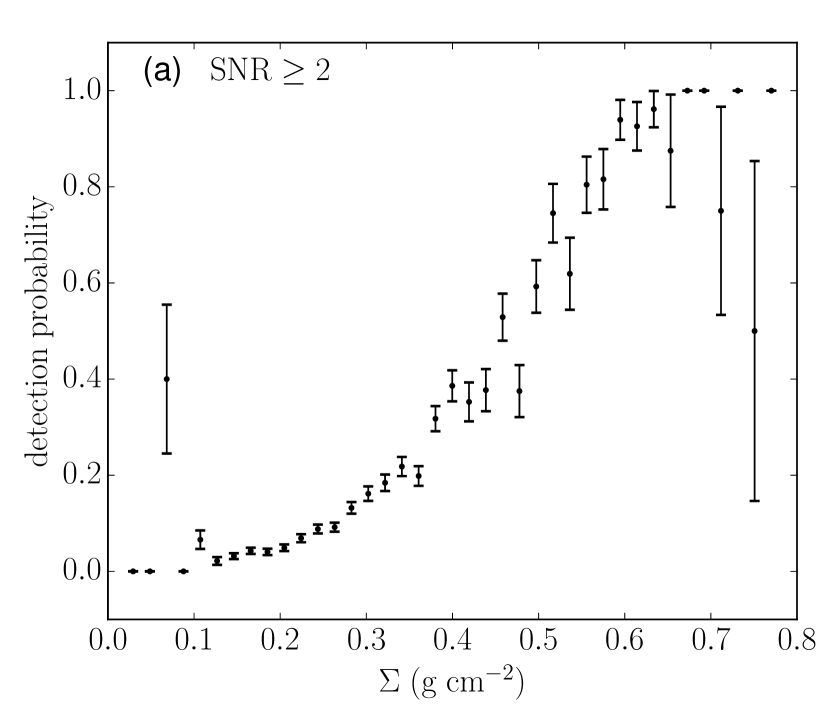
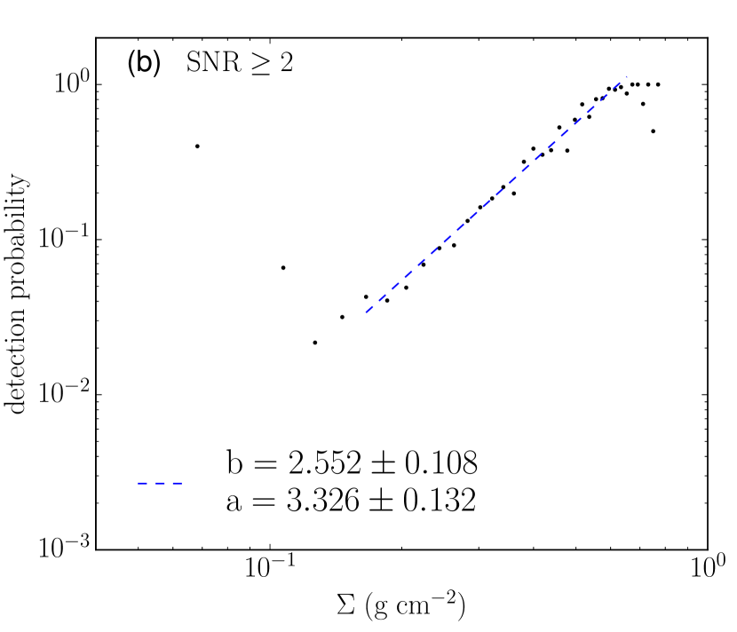
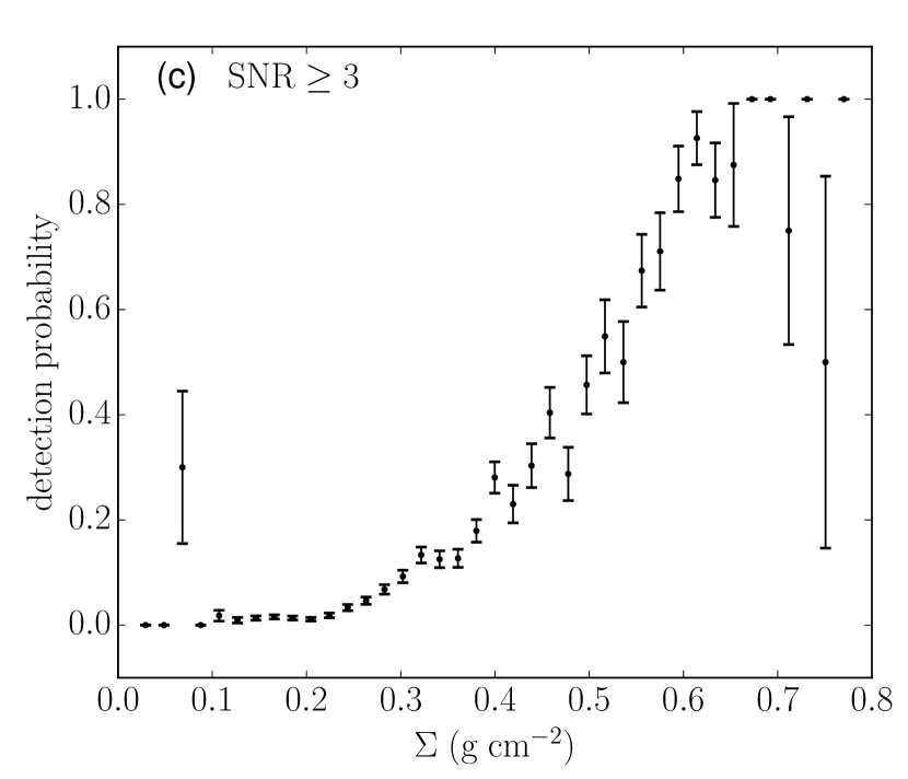
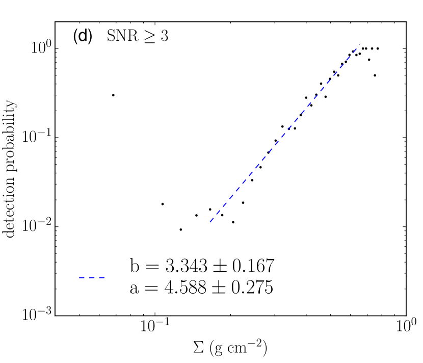
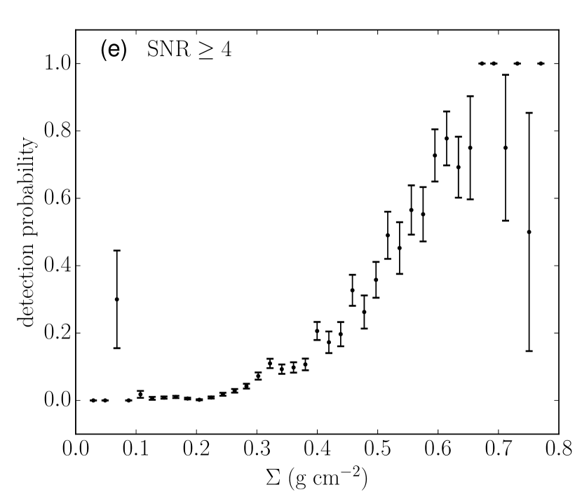
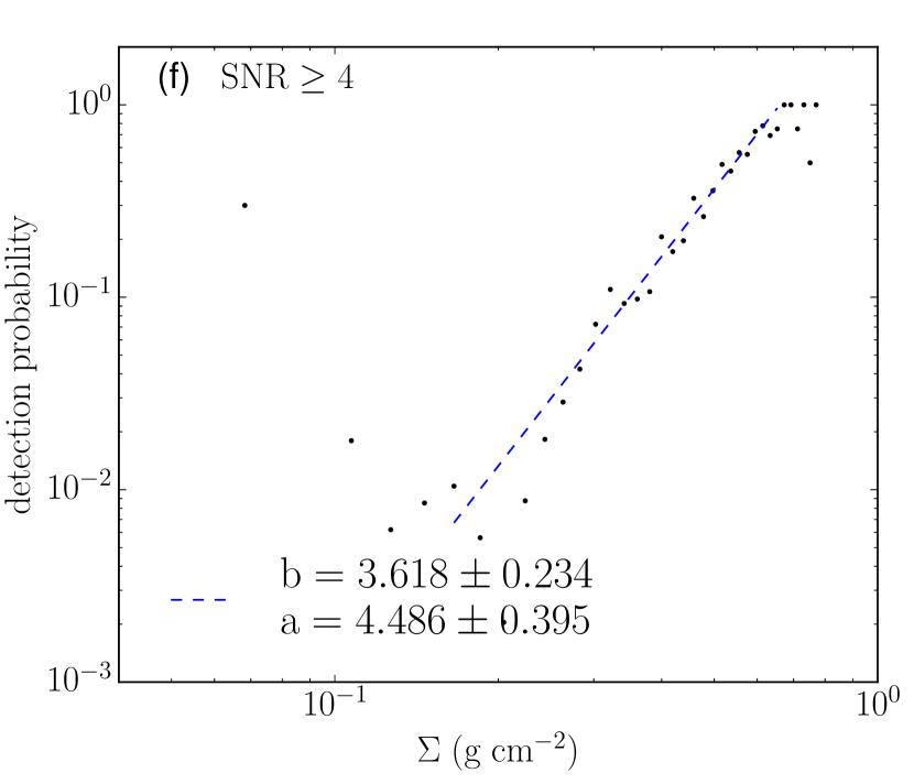
Figure 3.— (a): 1.3 mm continuum detection probability $P_{\rm 1.3mm}$ as a function of $\Sigma$. Here the continuum detection threshold is SNR = 2 with the RMS noise being 0.2 mJy per 2″ beam. The error bars are the square root of the variance of the Bernoulli distribution (see text). (b): The same as panel (a), but in logarithmic scale. The blue dashed line shows a power-law fit over the indicated range of $\Sigma$. The parameters $a$ and $b$ follow equation 3. (c): Same as (a), but with a detection threshold of SNR = 3. (d): Same as (c), but in logarithmic scale. (e): Same as (a), but with a detection threshold of SNR = 4. (f): Same as (e), but in logarithmic scale.

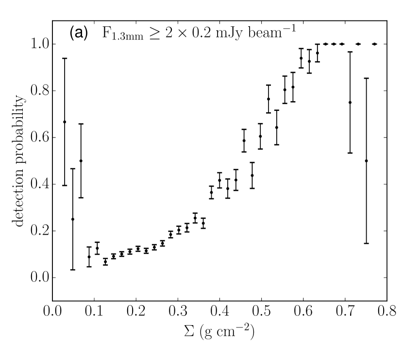
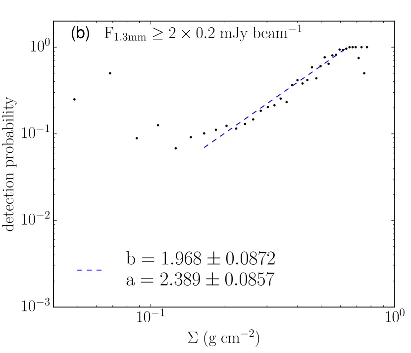
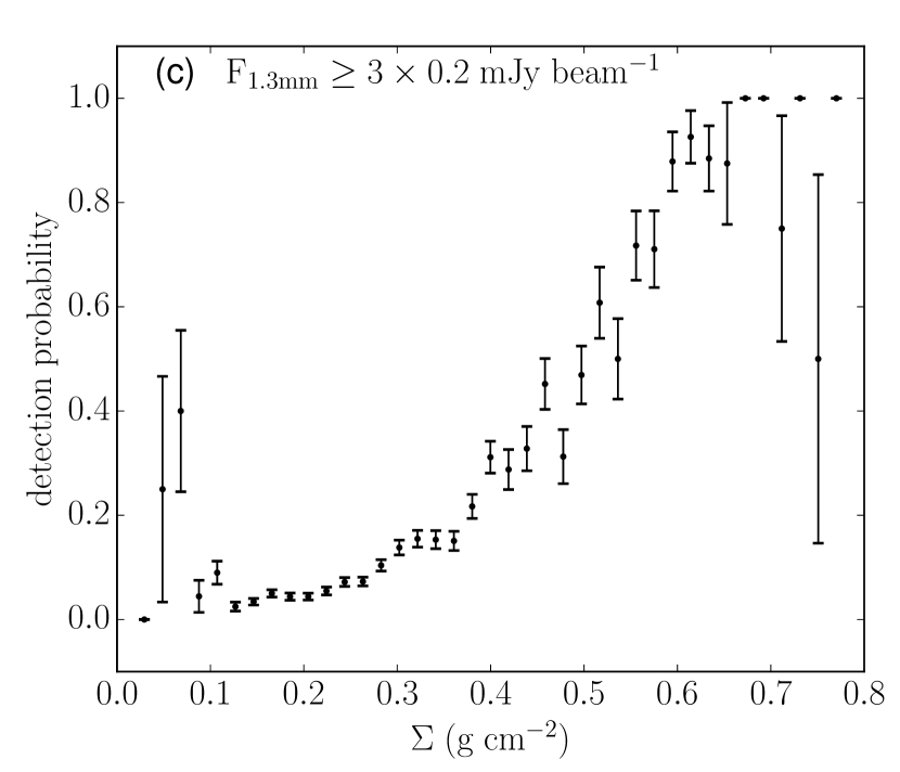
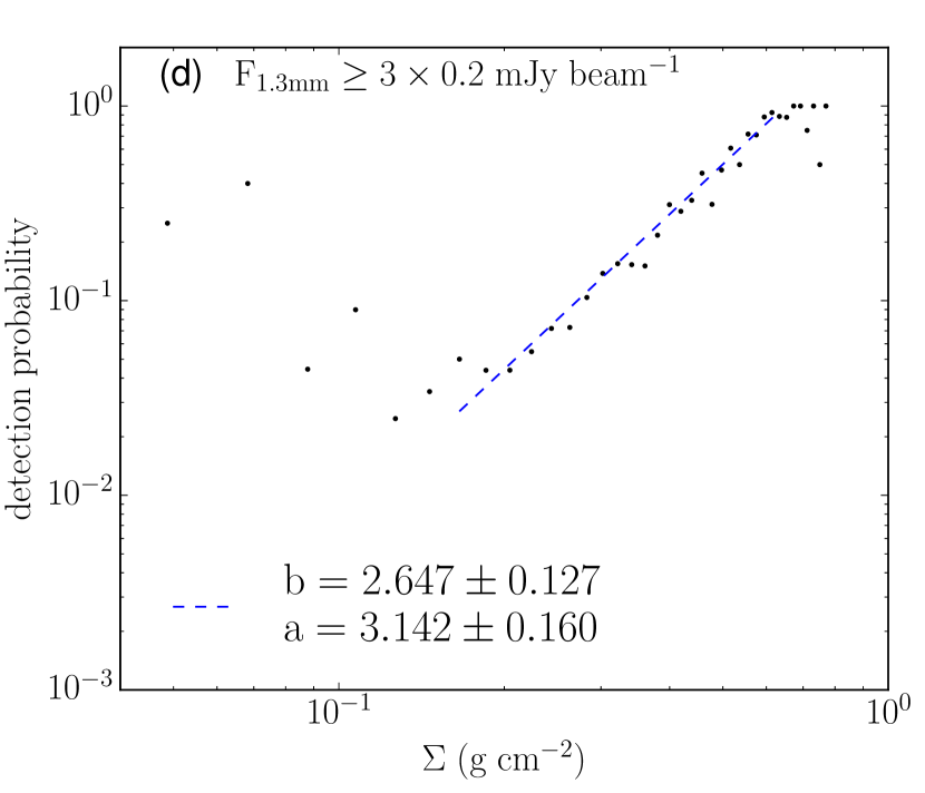
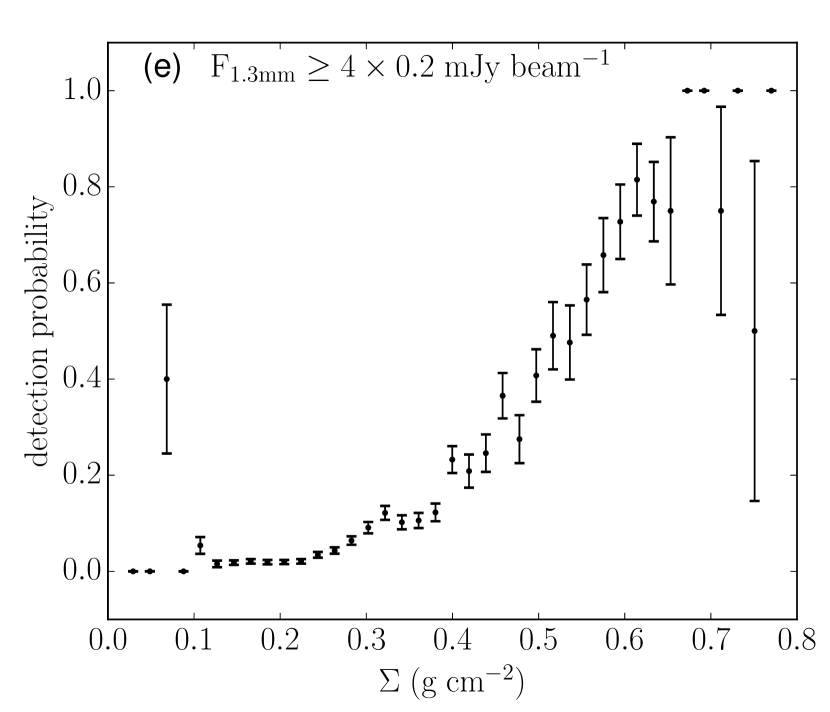
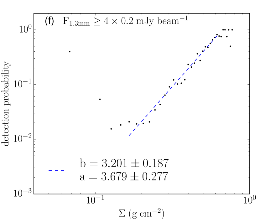
Figure 4.— (a): 1.3 mm continuum detection probability $P_{\rm 1.3mm}$ as a function of $\Sigma$. Here the continuum detection threshold is 2$\sigma_{\rm center}$, where $\sigma_{\rm center}$ (= 0.2 mJy per 2″ beam) is the RMS noise at map center (primary-beam response = 1). The error bars are the square root of the variance of the Bernoulli distribution (see text). (b): The same as panel (a), but in logarithmic scale. The blue dashed line shows a power-law fit over the indicated range of $\Sigma$. The parameters $a$ and $b$ follow equation 3. (c): Same as (a), but with a detection threshold of 3$\sigma_{\rm center}$. (d): Same as (c), but in logarithmic scale. (e): Same as panel (a), but with a detection threshold of 4$\sigma_{\rm center}$. (f): Same as panel (e), but in logarithmic scale.

To further quantify the relation between presence of 1.3 mm continuum emission and mass surface density of the parent cloud, we plot the detection probability, $P_{\rm 1.3mm}$, versus $\Sigma$ in Figures 3 and 4, using the dataset with pixels containing MIR sources removed (see above). Here $P_{\rm 1.3mm}$ is defined as the fraction of “detected” pixels at a given $\Sigma$. The definition of detection differs by cases. In the first case (Figure 3), a pixel is defined to be detected when its SNR is greater than a given threshold. A low threshold is more likely to have false detections, and vice versa. We adopt a fiducial threshold of SNR = 3, and show the effects from using SNR = 2 and SNR = 4. In the second case (Figure 4), a pixel is defined to be detected when its flux density is greater than a given threshold. Here we use the primary-beam corrected image. The fiducial threshold is 3$\sigma_{\rm center}$ at the map center, where the primary-beam response is 1. We also show the effects of using 2$\sigma_{\rm center}$ and 4$\sigma_{\rm center}$.

In the first case of a constant SNR threshold, it is possible that we miss some weak features at the map boundary where the RMS noise $\sigma$ is a factor of 2 higher than $\sigma_{\rm center}$. In the second case of a constant absolute flux density threshold, while this is closer to a constant physical limit, i.e., of constant core column density for fixed dust temperature and dust opacity, the disadvantage is that we may be overestimating $P_{\rm 1.3mm}$ near the map boundary due to increased contamination from noise fluctuations.

In these analyses, we adopt a bin size of $\Delta\Sigma$ = 0.02 g cm^-2 ($A_{V}\sim 4\>$mag). In the left columns of Figures 3 and 4, we show the $P_{\rm 1.3mm}-\Sigma$ relation with a linear scale. In the right columns, we show the relation with a logarithmic scale. Each row of panels shows the relation with a different detection threshold, as noted on the top-left corner.

In each $\Sigma$ bin, $P_{\rm 1.3mm}\equiv N_{\rm detection}/N_{\rm total}$. If each point obeys the Bernoulli distribution with success probability $p$, i.e.,

$${\rm P}(X)=\begin{cases}p&\text{if $X=1$}\\ 1-p&\text{if $X=0$}\\ \end{cases},$$ (2)

where $X=1$ means detection, then $P_{\rm 1.3mm}$ is the expectation of $\sum_{i=1}^{n}X_{i}/n$, given $X_{1}$…$X_{n}$ are independent, identically distributed random variables. The standard deviation of $\sum_{i=1}^{n}X_{i}/n$ is $[p(1-p)/n]^{0.5}$, which is adopted as the error bar for each bin. We use the observed probability as an estimate of the Bernoulli success probability. Note that by this method, estimating the error bar becomes problematic when the success probability equals 0 or 1. Such points are excluded from the functional fitting (see below).

At $\Sigma\lesssim 0.04\>\rm g~{}cm^{-2}$ ($A_{V}\sim 8\>$mag), there are very few (i.e., only about 5) pixels in the mapped region. While these pixels do not tend to show mm continuum flux detections via the various thresholds, there are too few for us to test scenarios of there being a threshold for star formation at about this level (e.g., McKee, 1989; Johnstone et al., 2004; Lada et al., 2010). Also, we note that the MIREX map, even with NIR extinction correction, can have relatively large systematic errors in this low-$\Sigma$ regime. Indeed, such problems, including incomplete removal of MIR sources, lead us to be cautious of results for $\Sigma\lesssim 0.15\>\rm g~{}cm^{-2}$, where $P_{\rm 1.3mm}$ is seen to sometimes have finite values, but typically with large errors.

However, in the main region of interest for our study, i.e., for $\Sigma\gtrsim 0.15\>\rm g~{}cm^{-2}$, in all the cases the detection probability increases steadily to reach approximately 100% by $\Sigma\sim 0.65~{}\rm g~{}cm^{-2}$. In Figures 3(b)(d)(f) and 4(b)(d)(f), the plots show that $P_{\rm 1.3mm}$ follows an approximate power-law relation with $\Sigma$ between $\Sigma\sim 0.15~{}\rm g~{}cm^{-2}$ and $\Sigma\sim 0.65~{}\rm g~{}cm^{-2}$. We fit the function $P_{\rm 1.3mm}=a(\Sigma/1\>\rm g~{}cm^{-2})^{b}$ by minimizing $\chi^{2}$ (normalized by the errors), which is shown as the blue dashed lines in these figures. Note, we do not include $P_{\rm 1.3mm}$ = 1 points in the fit. The resulting power-law indices $b$ and amplitudes $a$ are displayed in the figures and in Table 1.

With an increase in the level of the detection thresholds, Figures 3 and 4 show a decrease in detection probabilities, as expected. At the same time, the power-law indices become larger, i.e., with a higher detection threshold, the increase of $P_{\rm 1.3mm}$ between $\Sigma\sim 0.15~{}\rm g~{}cm^{-2}$ and $0.65~{}\rm g~{}cm^{-2}$ becomes steeper. In the next section we will use such power law approximations for $P_{\rm 1.3mm}(\Sigma)$ to estimate the mass fraction of “dense” gas in the IRDC and GMC region.

Table 1Detection Probability Relations

thresholds	$\Sigma_{\rm mm}\rm(g~{}cm^{-2})$	$a$	$b$	$f_{\rm dg,mm}$	$f_{\rm dg,MIREX}$	$f_{\rm dg,DPF,0.15-0.65}$	$f_{\rm dg,DPF,GMC}$
(1)	(2)	(3)	(4)	(5)(a)	(6)	(7)	(8)
SNR$\geq$2	0.029	3.3	2.6	10%${}_{6.0\%}^{15\%}$	20%	17%	9.2%
SNR$\geq$3	0.044	4.6	3.3	8.7%${}_{5.3\%}^{13\%}$	13%	12%	6.5%
SNR$\geq$4	0.058	4.5	3.6	8.0%${}_{4.9\%}^{12\%}$	10%	9.4%	5.7%
$F_{\rm 1.3mm}\geq 2\sigma_{\rm center}$	0.029	2.4	2.0	11%${}_{6.5\%}^{16\%}$	24%	22%	13%
$F_{\rm 1.3mm}\geq 3\sigma_{\rm center}$	0.044	3.1	2.6	9.5%${}_{5.8\%}^{14\%}$	17%	15%	8.2%
$F_{\rm 1.3mm}\geq 4\sigma_{\rm center}$	0.058	3.7	3.2	8.6%${}_{5.2\%}^{13\%}$	12%	11%	6.3%

• (a) The super- and subscripts correspond to using the lower (15 K) and higher (30 K) temperature assumptions in the mass estimation based on 1.3 mm continuum flux.

3.3. Dense Gas Fraction

The ALMA observations give us a direct measure of the amount of “dense” gas, i.e., that is detected by some defined criteria of 1.3 mm flux emission, which can be compared to the total mass estimate of the IRDC that overlaps with the region mapped by ALMA. From the MIREX map, this mass is $1.21\times 10^{4}\>M_{\odot}$, with uncertainties at the level of about 30% due to opacity per unit total mass uncertainties. Distance uncertainties contribute further, but these will cancel out in the ratio of these masses to the mm-continuum derived mass.

The total mm flux in the observed, analyzed region (i.e., where primary beam correction factor is $\leq 2$) is 1.42 Jy (based on detections above $3\sigma_{\rm center}$), which translates into a total mass of $1.16\times 10^{3}\>M_{\odot}$ given our fiducial assumptions, including $T=20\>$K. Thus the direct measure of dense gas mass fraction (expressed as percentages) is $f_{\rm dg,mm}=9.5\%$ for this case. This value is listed in column (5) of Table 1 for all the considered cases, and showing the effects of varying $T$ from 15 K to 30 K. We see the sensitivity of these dense gas fractions to threshold choice and temperature choice, with fiducial results being about 10%. Systematic variations arising from the choice of dust temperature are up to a factor of almost two and are the most significant source of uncertainty (see also Goodman et al., 2009).

A second estimate of the dense gas fraction, $f_{\rm dg,MIREX}$ can be made by summing the MIREX mass estimate of the pixels that are detected in 1.3 mm continuum. These values are shown in column (6) of Table 1. Fiducial results are now moderately higher at about 15%.

Next we utilize our analytic approximations for the detection probability function (DPF), $P_{\rm 1.3mm}(\Sigma)$, combined with analytic forms for the probability distribution function (PDF) of $\Sigma$ to estimate dense gas fractions. Recall, the observed DPFs have a power law form in the range from $\Sigma\sim 0.15\rm g~{}cm^{-2}$ to $\sim 0.65\rm g~{}cm^{-2}$. At lower values of $\Sigma$ we extrapolate with a constant that is similar to the $P_{\rm 1.3mm}$ at $\Sigma=0.15\>\rm g~{}cm^{-2}$. Finally at high values, $\Sigma>0.65\rm g~{}cm^{-2}$ we use a constant value of unity. Thus, overall the DPF is described via

$$P_{\rm 1.3mm}=\begin{cases}P_{\rm 1.3mm,min}&\text{if $\Sigma/({\rm g~{}cm}^{-2})<0.15$}\\ a(\frac{\Sigma}{1~{}\rm g~{}cm^{-2}})^{b}&\text{if $0.15<\Sigma/({\rm g~{}cm}^{-2})<0.65$}\\ 1&\text{if $\Sigma/({\rm g~{}cm}^{-2})>0.65$},\\ \end{cases}$$ (3)

where $P_{\rm 1.3mm,min}=a(0.15~{}\rm g~{}cm^{-2}/1~{}\rm g~{}cm^{-2})^{b}$. The fiducial value for $P_{\rm 1.3mm,min}$ is $\sim 0.02$. This value acts effectively as a lower limit floor on our estimated values of $f_{\rm dg}$.

Then the mass of dense, i.e., 1.3mm-emitting, gas is

$$M_{\rm dg}=\int P_{\rm 1.3mm}\Sigma Ap({\rm ln}\Sigma){\rm d(ln}\Sigma)$$ (4)

where $A$ is the total cloud area being integrated over and $p({\rm ln}\Sigma)$ is the cloud’s PDF of mass surface densities.

Based on two independent methods, the $\Sigma$-PDF in IRDC G28.37+0.07 and its surroundings (i.e., of a $\sim 20\arcmin$-scale region, equivalent to $\sim 30\>$pc) has been found to be reasonably well fit by a single log-normal function (Butler et al., 2014; Lim et al., 2016), i.e., of the form

$$p(\rm ln\Sigma)=\frac{1}{\sqrt{2\pi}\sigma_{\rm ln\Sigma}}\rm exp[-\frac{(\rm ln\Sigma-\overline{\rm ln\Sigma})^{2}}{2\sigma_{\rm ln\Sigma}^{2}}].$$ (5)

Here we adopt this empirical $\Sigma$-PDF (i.e., area-weighted) in the NIR+MIR extinction map case, i.e., with $\sigma_{\rm ln\Sigma}$ = 1.15, $\overline{\rm\Sigma}$ = 0.038 $\rm g~{}cm^{-2}$, and $\overline{\rm ln\Sigma}$ = -3.93. We note that the actual $\Sigma$-PDF measured by Lim et al. (2016) has a small power law tail excess component, emerging at about $\Sigma\sim 0.3\>{\rm g\>cm}^{-2}$. While the use of the above log-normal leads to a small underestimation of the importance of the higher $\Sigma$ regions, it is a very modest effect since the fraction of pixels affected by this excess is less than a few percent.

Then the total mass of dense gas can be estimated by integrating equation 4. If we carry out this exercise for the area corresponding to the analyzed area of the IRDC, i.e., that mapped by ALMA with a primary beam response $>0.5$, we obtain 135$\>M_{\odot}$. This is much smaller than our previous estimates for $M_{\rm dg}$, which is primarily because the $\Sigma$-PDF was estimated for a much larger region and contains much more contribution from lower values of $\Sigma$. If we restrict the above integration to the range $\Sigma=0.15$ to $0.65\>{\rm g\>cm}^{-2}$, then we obtain $M_{\rm dg}=1,828\>M_{\odot}$ (for the $>3\sigma_{\rm center}$ case), in much closer agreement with our previous estimates. Dense gas fractions calculated via this latter method can be derived by comparison to the total cloud mass observed in the mapped region, i.e., $1.21\times 10^{4}\>M_{\odot}$, yielding the values $f_{\rm dg,DPF,0.15-0.65}$ in column (7) of Table 1. These values are very similar to those of $f_{\rm dg,MIREX}$.

Finally, we can make the extrapolation that the observed DPF of the inner IRDC region mapped by ALMA will hold in the wider GMC region, where the approximately log-normal $\Sigma$-PDF was measured. For this $\sim 30\>$pc-scale region, the total cloud mass is

$$M_{\rm tot}=\int\Sigma Ap({\rm ln}\Sigma){\rm d(ln}\Sigma),$$ (6)

which has a value of 170,000$\>M_{\odot}$. The values of $f_{\rm dg,DPF,GMC}=M_{\rm dg}/M_{\rm tot}$ are shown in column (8) of Table 1. In the fiducial cases, these values are smaller than 10%.

4. Discussion

4.1. Core/Star Formation Efficiency

The MIR extinction map and the ALMA 1.3 mm continuum map both trace dust in the IRDC, which are then used to estimate the masses. However, while the MIREX map traces the total mass surface density without bias at any particular spatial scale and without bias on the temperature (as long as the region is cold enough not to be emitting at $\rm 8\>\mu m$), the ALMA continuum map misses flux from extended structures ($\gtrsim 20\arcsec$) and is biased towards warmer material. We describe the mass associated with the 1.3 mm continuum flux as the “dense” gas component and discuss below that the majority of this material is likely to be directly involved in the star formation process.

We have measured the mass of the component that is detected by our ALMA observation of dust continuum emission and find it to be about $f_{\rm dg,mm}\sim$10% of the total mass in the “central”, i.e., mapped region of the IRDC, but with about 50% uncertainties due to assumed dust temperature. If we use the values of the MIREX pixels at the locations where mm continuum emission is seen, then the associated mass fraction increases by a factor of about 1.7 (depending on the choice of flux threshold), i.e., to $f_{\rm dg,MIREX}\sim$17%. The difference between $f_{\rm dg,MIREX}$ and $f_{\rm dg,mm}$ could be due to, e.g., a dense core filling factor of less than one on the scale of the 2″ pixels or a systematically lower temperature of the mm continuum emitting dust, i.e., $\sim 15\>$K rather than $20\>$K.

If we use the data to define a detection probability of mm continuum emission as a function of $\Sigma$ and then apply this to an estimate of the $\Sigma$-PDF of the mapped region of the IRDC, i.e., a log-normal but restricted to the range of $\Sigma=0.15$ to $0.65\>{\rm g\>cm}^{-2}$, then we obtain values of dense gas fractions of $f_{\rm dg,DPF,0.15-0.65}\simeq$15%, very similar to the values of $f_{\rm dg,MIREX}$ (also compare other values in columns 6 and 7), which indicates that the analytic approximations for the DPF are quite accurate. Extrapolating the observed DPF of the inner IRDC region to the wider GMC region, where the $\Sigma$-PDF was seen to be well-fit by a single log-normal (BTK14; Lim et al., 2016), then integration with this PDF leads to estimates of $f_{\rm dg,DPF,GMC}\simeq$8%. We note that this mass fraction is very similar to the mass fraction of the GMC that is in the power law tail part of the $\Sigma$-PDF, $\epsilon_{\rm pl}\sim$3% to 8% (Lim et al., 2016) based on lower angular resolution Herschel measurements of sub-mm dust continuum emission from the region.

Our ALMA continuum map detects the C1a, C1-Sa, and C1-Sb protostellar cores from Tan et al. (2016), which includes some lower-mass objects. It also detects the five main continuum structures in C2 (Zhang et al., 2009, 2015), which have been resolved into a population of cores extending down to sub-solar masses. Thus it is likely that the current observations capture a significant fraction of the core mass function (CMF) of protostellar cores. The detected mm flux may also contain some contribution from more massive pre-stellar cores, such as C1-S and C1-N (Tan et al., 2013; Kong et al., 2017). Thus, for simplicity, we will assume that our detected 1.3 mm continuum fluxes give a near complete census of the protostellar CMF and ignore the possibility that it may include some contribution from the pre-stellar CMF. These effects of protostellar CMF incompleteness and pre-stellar CMF contribution will offset each other to some extent. Under this assumption, then the total current star-forming core efficiency is simply the same as $f_{\rm dg}$. If we next further assume that the star formation efficiency from individual cores is about 50%, which is expected based on models of outflow feedback (Matzner & McKee, 2000; Zhang et al., 2014), then the total mass of stars that would form from the currently observed cores is about half of $f_{\rm dg}$, i.e., $\epsilon_{*}\sim$5% to $\sim$8%.

4.2. Star Formation Rates

A number of star formation models involve protostellar cores collapsing at rates similar to their local free-fall rate (e.g., Shu et al., 1987; McKee & Tan, 2003; Krumholz & McKee, 2005). The Turbulent Core Model (McKee & Tan, 2003, hereafter MT03) assumes core properties are set by the mean pressure in their surrounding, self-gravitating clump, which then leads to a simple relation between the individual star formation time and the average free-fall time of the clump. In the fiducial case the timescale for star formation is $t_{*f}=1.3\times 10^{5}(M_{c}/60\>M_{\odot})^{1/4}(\Sigma_{\rm cl}/1\>{\rm g\>cm}^{-2})^{-3/4}\>{\rm yr}$ (cf. equation 44 in MT03), which has a very weak dependence on core mass, $M_{c}$, and clump mass surface density, $\Sigma_{\rm cl}$. This timescale is related to the clump’s mean free-fall time via $t_{*f}/\bar{t}_{\rm ff,cl}=0.98(M_{c}/60\>M_{\odot})^{1/4}(M_{\rm cl}/4000\>M_{\odot})^{-1/4}$ (cf. equation 37 in MT03), i.e., they are quite similar.

For a CMF that is a Salpeter (1955) power law of form $dN/d{\rm log}M_{c}\propto M_{c}^{-\alpha}$ with $\alpha=1.35$ with lower limit of $M_{c}=1\>M_{\odot}$ and upper limit of $240\>M_{\odot}$ (so that resulting stellar IMF with 50% formation efficiency from the core is in the range from $m_{*}=0.5\>M_{\odot}$ to $120\>M_{\odot}$, which is, for our purposes, a reasonable approximation of the actual observed IMF), then half of the mass of the core population has $M_{c}\gtrsim 5\>M_{\odot}$. Thus we take $M_{c}=5\>M_{\odot}$ as a typical core mass. The mapped region of the IRDC has a total mass of $\simeq 1.21\times 10^{4}\>M_{\odot}$, which we will approximate as $10^{4}\>M_{\odot}$. Under these two conditions, $t_{*f}/\bar{t}_{\rm ff,cl}\rightarrow 0.42$.

Assuming the SFR is steady and the CMF is evenly populated, then the observed cores will represent those objects that have formed in the last average individual star formation time, $\bar{t}_{*f}$, i.e., the last $0.42\bar{t}_{\rm ff,cl}$. Taking the mass fraction in dense gas (defined at $F_{\rm 1.3mm}\geq 3\sigma_{\rm center}$) as $f_{\rm dg,mm}=0.095^{0.14}_{0.058}$ as the most accurate estimate of the current mass fraction in protostellar cores in the observed region of the IRDC, then we find that, for $\epsilon_{\rm core}=0.5$ (Matzner & McKee, 2000; Zhang et al., 2014), the star formation efficiency per free-fall time is $\epsilon_{\rm ff}=0.11^{0.17}_{0.069}$.

This estimate of $\epsilon_{\rm ff}\sim 0.1$ is about a factor of two larger than the value estimate inside the half-mass radius of the Orion Nebula Cluster by Da Rio et al. (2014), which was estimated from observed age spreads of young stellar objects. However, the uncertainties arising solely from the uncertain temperatures of protostellar cores (15 to 30 K range adopted here) lead to almost a factor of two uncertainty in $\epsilon_{\rm ff}$. The mean mass surface density in the analyzed region of the IRDC is $\simeq 0.26\>{\rm g\>cm}^{-2}$. The protostellar core models of Zhang & Tan (2015), i.e., for $M_{c}=2,3,4\>M_{\odot}$, in $\Sigma\simeq 0.3\>{\rm g\>cm}^{-2}$ clump environments have mean envelope temperatures near 20 K (set mostly by accretion luminosities), but can exceed 30 K in $\Sigma\simeq 1\>{\rm g\>cm}^{-2}$ regions that have higher accretion rates. Also, more massive cores forming more massive protostars, will tend to have warmer envelope temperatures, which would lower our estimates of the mass of the core population and thus $\epsilon_{\rm ff}$. These uncertainties can be reduced by carrying out temperature measurements of each protostellar core (e.g., of the dust via spectral energy distribution observations and modeling or of associated gas via, e.g., $\rm NH_{3}$ observations).

In addition to the effects of core temperature uncertainties, additional systematic uncertainties include that the analysis has assumed a fixed value of the star formation efficiency from the core, a particular relation between star formation time and clump free-fall time (fiducial case from MT03) and equates the observed 1.3 mm continuum structures with the total protostellar core population. These assumptions and uncertainties can be improved with future work. For example, observations of CO outflows can be used to confirm that mm continuum sources are indeed protostellar cores. Better sensitivity of mm continuum data can help to probe further down the protostellar CMF (although with the half-mass point estimated to be near $5\>M_{\odot}$, we expect that the bulk of the population containing most of the mass has already been detected). Assumptions about star formation efficiency from the core can be tested with improved theoretical and numerical models (e.g., Tanaka et al., 2017; Matsushita et al., 2017). The relation of individual star formation time to mean clump free-fall time is more difficult to test observationally, and may depend on the uncertain degree of magnetization in the cores (Li & Shu, 1997, MT03). One observational test involves measuring the mass accretion rates of the protostars, potentially from modeling their spectral energy distributions (see, e.g., De Buizer et al., 2017; Zhang & Tan, 2015, 2017) or from measuring their mass outflow rates that are expected to be proportional to accretion rates (see, e.g., Beltrán & de Wit, 2016).

5. Conclusions

In this paper, we have presented first results from an ALMA 1.3 mm continuum mosaic observation using the 12-m array of the central regions of a massive IRDC, which is a potential site of massive star cluster formation. We have focused on carrying out a detailed comparison of the 1.3 mm emission (which is sensitive to structures $\lesssim 20\arcsec$ in size) with a MIR-derived extinction map of the cloud. In particular, we argue that the 1.3 mm structures likely trace “dense”, protostellar cores, and have studied the prevalence of such sources in the IRDC as a function of its local mass surface density, $\Sigma$. Based on various definitions of 1.3 mm continuum detection, i.e., at a fixed signal to noise ratio or a fixed absolute flux density, we find that the detection probability function (DPF), $P_{\rm 1.3mm}(\Sigma)$, rises as a power law, i.e., $\propto(\Sigma/1\>{\rm g\>cm}^{-2})^{b}$ with $b\sim 3$ in the fiducial cases, over the range $0.15\lesssim\Sigma/1\>{\rm g\>cm}^{-2}\lesssim 0.65$. At higher values of $\Sigma$, we find that $P_{\rm 1.3mm}\simeq 1$. At lower values of $\Sigma$, which are not so common in the mapped region, we have weaker constraints on $P_{\rm 1.3mm}$, but approximate it as a constant of $\sim 10^{-2}$ in the fiducial cases. Such an empirical relation can provide a test of theoretical/numerical models of star formation.

We have then utilized the continuum image and the estimated form of $P_{\rm 1.3mm}(\Sigma)$ to carry out various estimates of the “dense” gas mass fraction, $f_{\rm dg}$, in the IRDC and, by extrapolation with the observed $\Sigma$-PDF, in the larger-scale GMC region. The mass estimate in the mapped region of the IRDC made directly from the observed 1.3 mm flux depends on adopted dust opacities and temperatures, but has a fiducial value of just under 10%. Using the MIREX $\Sigma$ at location of 1.3 mm flux detection leads to mass fraction estimates that are about a factor of 1.5 times higher. Extrapolating to the larger scale region, given its observed log-normal $\Sigma$-PDF, we find values of $f_{\rm dg}\sim 7\%$.

Finally, assuming that the detected 1.3 mm structures mostly trace protostellar cores and capture the bulk of the mass of the core population, we use these results to estimate the star formation rate in the IRDC, in particular the star formation efficiency per free-fall time, $\epsilon_{\rm ff}$. This analysis requires a model to link core properties to ambient clump properties, for which we utilize the Turbulent Core Model of McKee & Tan (2003). Then individual star formation times are, on average, about half of the clump free-fall time. Given an expected core to star formation efficiency, $\epsilon_{\rm core}$, of about 50%, then leads to estimates of $\epsilon_{\rm ff}\simeq f_{\rm dg}\simeq 10\%$.

Future improvements in this measurement have been outlined, including better temperature and thus mass estimates of the protostellar cores and confirmation of protostellar activity via analysis of outflow properties. Future work may also include extension of these methods to a larger sample of IRDCs and star-forming regions.

References

- Alves et al. (2017) Alves, J., Lombardi, M., & Lada, C. J. 2017, A&A, 606, L2
- André et al. (2014) André, P., Di Francesco, J., Ward-Thompson, D., et al. 2014, Protostars and Planets VI, 27
- Beltrán & de Wit (2016) Beltrán, M. T., & de Wit, W. J. 2016, A&A Rev., 24, 6
- Bergin & Tafalla (2007) Bergin, E. A., & Tafalla, M. 2007, ARA&A, 45, 339
- Butler & Tan (2009) Butler, M. J., & Tan, J. C. 2009, ApJ, 696, 484
- Butler & Tan (2012) —. 2012, ApJ, 754, 5
- Butler et al. (2014) Butler, M. J., Tan, J. C., & Kainulainen, J. 2014, ApJ, 782, L30
- Chabrier et al. (2014) Chabrier, G., Hennebelle, P., & Charlot, S. 2014, ApJ, 796, 75
- Chen et al. (2017) Chen, H., Burkhart, B., Goodman, A. A., & Collins, D. C. 2017, ArXiv e-prints, arXiv:1707.09356
- Christie et al. (2017) Christie, D., Wu, B., & Tan, J. C. 2017, ApJ, 848, 50
- Churchwell et al. (2009) Churchwell, E., Babler, B. L., Meade, M. R., et al. 2009, PASP, 121, 213
- Collins et al. (2011) Collins, D. C., Padoan, P., Norman, M. L., & Xu, H. 2011, ApJ, 731, 59
- Da Rio et al. (2014) Da Rio, N., Tan, J. C., & Jaehnig, K. 2014, ApJ, 795, 55
- De Buizer et al. (2017) De Buizer, J. M., Liu, M., Tan, J. C., et al. 2017, ApJ, 843, 33
- Draine (2011) Draine, B. T. 2011, Physics of the Interstellar and Intergalactic Medium, Princeton Series in Astrophysics (Princeton University Press)
- Federrath & Klessen (2013) Federrath, C., & Klessen, R. S. 2013, ApJ, 763, 51
- Goodman et al. (2009) Goodman, A. A., Pineda, J. E., & Schnee, S. L. 2009, ApJ, 692, 91
- Hennebelle & Chabrier (2008) Hennebelle, P., & Chabrier, G. 2008, ApJ, 684, 395
- Hennebelle & Chabrier (2011) —. 2011, ApJ, 743, L29
- Johnstone et al. (2004) Johnstone, D., Di Francesco, J., & Kirk, H. 2004, ApJ, 611, L45
- Kainulainen et al. (2009) Kainulainen, J., Beuther, H., Henning, T., & Plume, R. 2009, A&A, 508, L35
- Kainulainen & Tan (2013) Kainulainen, J., & Tan, J. C. 2013, A&A, 549, A53
- Kennicutt & Evans (2012) Kennicutt, R. C., & Evans, N. J. 2012, ARA&A, 50, 531
- Kong et al. (2017) Kong, S., Tan, J. C., Caselli, P., et al. 2017, ArXiv e-prints, arXiv:1701.05953
- Krumholz et al. (2012) Krumholz, M. R., Klein, R. I., & McKee, C. F. 2012, ApJ, 754, 71
- Krumholz & McKee (2005) Krumholz, M. R., & McKee, C. F. 2005, ApJ, 630, 250
- Krumholz & Tan (2007) Krumholz, M. R., & Tan, J. C. 2007, ApJ, 654, 304
- Kunz & Mouschovias (2009) Kunz, M. W., & Mouschovias, T. C. 2009, MNRAS, 399, L94
- Lada et al. (2010) Lada, C. J., Lombardi, M., & Alves, J. F. 2010, ApJ, 724, 687
- Lee et al. (2016) Lee, E. J., Miville-Deschênes, M.-A., & Murray, N. W. 2016, ApJ, 833, 229
- Li & Shu (1997) Li, Z.-Y., & Shu, F. H. 1997, ApJ, 475, 237
- Lim et al. (2016) Lim, W., Tan, J. C., Kainulainen, J., Ma, B., & Butler, M. J. 2016, ApJ, 829, L19
- Lombardi (2009) Lombardi, M. 2009, A&A, 493, 735
- Matsushita et al. (2017) Matsushita, Y., Machida, M. N., Sakurai, Y., & Hosokawa, T. 2017, MNRAS, 470, 1026
- Matzner & McKee (2000) Matzner, C. D., & McKee, C. F. 2000, ApJ, 545, 364
- McKee (1989) McKee, C. F. 1989, ApJ, 345, 782
- McKee & Tan (2003) McKee, C. F., & Tan, J. C. 2003, ApJ, 585, 850
- Murray (2011) Murray, N. 2011, ApJ, 729, 133
- Myers (2015) Myers, P. C. 2015, ApJ, 806, 226
- Offner et al. (2014) Offner, S. S. R., Clark, P. C., Hennebelle, P., et al. 2014, Protostars and Planets VI, 53
- Ossenkopf & Henning (1994) Ossenkopf, V., & Henning, T. 1994, A&A, 291, 943
- Padoan & Nordlund (2002) Padoan, P., & Nordlund, Å. 2002, ApJ, 576, 870
- Padoan & Nordlund (2011) —. 2011, ApJ, 741, L22
- Sanhueza et al. (2017) Sanhueza, P., Jackson, J. M., Zhang, Q., et al. 2017, ApJ, 841, 97
- Scoville et al. (1986) Scoville, N. Z., Sanders, D. B., & Clemens, D. P. 1986, ApJ, 310, L77
- Shu et al. (1987) Shu, F. H., Adams, F. C., & Lizano, S. 1987, ARA&A, 25, 23
- Stutz & Kainulainen (2015) Stutz, A. M., & Kainulainen, J. 2015, A&A, 577, L6
- Tan (2000) Tan, J. C. 2000, ApJ, 536, 173
- Tan (2016) Tan, J. C. 2016, in IAU Symposium, Vol. 315, From Interstellar Clouds to Star-Forming Galaxies: Universal Processes?, ed. P. Jablonka, P. André, & F. van der Tak, 154–162
- Tan et al. (2014) Tan, J. C., Beltrán, M. T., Caselli, P., et al. 2014, Protostars and Planets VI, 149
- Tan et al. (2013) Tan, J. C., Kong, S., Butler, M. J., Caselli, P., & Fontani, F. 2013, ApJ, 779, 96
- Tan et al. (2016) Tan, J. C., Kong, S., Zhang, Y., et al. 2016, ApJ, 821, L3
- Tanaka et al. (2017) Tanaka, K. E. I., Tan, J. C., & Zhang, Y. 2017, ApJ, 835, 32
- Wu et al. (2017) Wu, B., Tan, J. C., Christie, D., et al. 2017, ApJ, 841, 88
- Wu et al. (2015) Wu, B., Van Loo, S., Tan, J. C., & Bruderer, S. 2015, ApJ, 811, 56
- Zhang et al. (2015) Zhang, Q., Wang, K., Lu, X., & Jiménez-Serra, I. 2015, ApJ, 804, 141
- Zhang et al. (2009) Zhang, Q., Wang, Y., Pillai, T., & Rathborne, J. 2009, ApJ, 696, 268
- Zhang & Tan (2015) Zhang, Y., & Tan, J. C. 2015, ApJ, 802, L15
- Zhang & Tan (2017) —. 2017, ArXiv e-prints, arXiv:1708.08853
- Zhang et al. (2014) Zhang, Y., Tan, J. C., & Hosokawa, T. 2014, ApJ, 788, 166
- Zuckerman & Evans (1974) Zuckerman, B., & Evans, II, N. J. 1974, ApJ, 192, L149