Mass functions from the excursion set model

Abstract

Aims. We aim to study the stochastic evolution of the smoothed overdensity $\delta$ at scale $S$ of the form $\delta(S)=\int_{0}^{S}K(S,u)\mathrm{d}W(u)$, where $K$ is a kernel and $\mathrm{d}W$ is the usual Wiener process.

Methods. For a Gaussian density field, smoothed by the top-hat filter, in real space, we used a simple kernel that gives the correct correlation between scales. A Monte Carlo procedure was used to construct random walks and to calculate first crossing distributions and consequently mass functions for a constant barrier.

Results. We show that the evolution considered here improves the agreement with the results of N-body simulations relative to analytical approximations which have been proposed from the same problem by other authors. In fact, we show that an evolution which is fully consistent with the ideas of the excursion set model, describes accurately the mass function of dark matter haloes for values of $\nu\leq 1$ and underestimates the number of larger haloes. Finally, we show that a constant threshold of collapse, lower than it is usually used, it is able to produce a mass function which approximates the results of N-body simulations for a variety of redshifts and for a wide range of masses.

Conclusions. A mass function in good agreement with N-body simulations can be obtained analytically using a lower than usual constant collapse threshold.

1 Introduction

Over the course of the past several decades, cosmologists using a large number of observations came up with a model describing the structure and evolution of the universe, dubbed $\Lambda$CDM model. In this model the Universe is constituted by cold dark matter (CDM), and vacuum energy (represented by the cosmological constant $\Lambda$). This model fits a large number of data (Del Popolo, 2007; Komatsu et al., 2011; Del Popolo, 2013, 2014; Planck Collaboration XIII, 2016), but suffers from drawbacks on small scales (see Del Popolo & Le Delliou, 2017), the fine tuning problem (Weinberg, 1989; Astashenok & del Popolo, 2012) and the cosmic coincidence problem. Another fundamental test that the $\Lambda$CDM model has to pass is to accurately predict the dark matter (DM) haloes distribution (i.e., the halo mass function (MF) (see Del Popolo & Yesilyurt, 2007; Hiotelis & Del Popolo, 2006; Hiotelis & del Popolo, 2013)). The high mass end of the MF at small redshift ( $z\leq 2$) is very sensitive to cosmological parameters like the Universe matter and dark energy (DE) content ($\Omega_{\rm m}$ and $\Omega_{\Lambda}$), the equation of state of the Universe, $w$, and its evolution (Malekjani et al., 2015; Pace et al., 2014). At redshifts higher than the previously quoted ones, the MF is of fundamental importance in the study of the reionization history of the universe (e.g., Furlanetto et al., 2006), quasar abundance (e.g., Haiman & Loeb, 2001), and to study the distribution of DM.

Press & Schechter (1974) (PS) proposed a very simple model based on the assumption of Gaussian distribution of the initial density perturbation, and the spherical collapse model. The quoted approach has the drawback of overpredicting the number of objects at small masses, and underpredicting those at high mass (e.g., Jenkins et al., 2001; White, 2002). The extended-PS formalism, or excursion set approach, (Bond et al., 1991; Bower, 1991; Lacey & Cole, 1993; Gardner, 2001), introduced to overcome the quoted problems, was unable to solve them.

Extension of the quoted formalism (Del Popolo & Gambera, 1998, 1999, 2000; Sheth et al., 2001), moving from the spherical collapse to non-spherical collapse gave much better agreement with N-body simulations (Sheth & Tormen, 1999) (ST). However, a deeper analysis of ST, and Sheth et al. (2001) showed that the ST MF overpredicts the halo number at large masses (Warren et al., 2006; Lukić et al., 2007; Reed et al., 2007; Crocce et al., 2010; Bhattacharya et al., 2011; Angulo et al., 2012; Watson et al., 2013), and when the redshift evolution is studied the situation worsen (Reed et al., 2007; Lukić et al., 2007; Courtin et al., 2011).

Another important issue is that of the universality of the MF, namely its independence on cosmology and redshift. Several studies (e.g., Tinker et al., 2008; Crocce et al., 2010; Bhattacharya et al., 2011; Courtin et al., 2011; Watson et al., 2013) showed that the MF is not universal nor in its $z$ dependence or for different cosmologies.

In the present paper, we want to show how the excursion set approach can be improved to the extent that it can produce a MF in good agreement with N-body simulations like that of (Tinker et al., 2008) who showed clear evidences of the MF deviations from universality, calibrated the MF at $z=0$ in the $10^{11}<M<10^{15}\leavevmode\nobreak\ h^{-1}\leavevmode\nobreak\ M_{\odot}$ mass range within 5%, and found the redshift evolution of the same.

The paper is organized as follows. In Sect. 2, we discuss the stochastic process, and Sect. 3 is devoted to results and discussion.

2 The stochastic process.

As already reported, the excursion set model is based on the ideas of Press & Schechter (1974) and on their extensions which are presented in the pioneered works of Bond et al. (1991) and Lacey & Cole (1993). We will improve on these ideas in this paper but before that we will write some useful relations about the density fields and the smoothing filters which will be used in what follows.
The smoothed density perturbation at the center of a spherical region is

$$\delta(R)=\int W_{f}(r;R)\hat{\delta}(r)4\pi r^{2}\mathrm{d}r,$$ (1)

where $\hat{\delta}(r)$ is the density at distance $r$ from the center of the spherical region and $W_{f}$ is a smoothing filter. Reducing $R$, the variable $\delta$ executes a random walk that depends on the form of the density field and on the smoothing filter $W_{f}$. If the density field is Gaussian, then $\delta$ is a central Gaussian variable and its probability density is given by

$$p(\delta(R)=x)\mathrm{d}x=\frac{1}{\sqrt{2\pi\sigma^{2}(R)}}\mathrm{exp}\left[-\frac{x^{2}}{2\sigma^{2}(R)}\right]\mathrm{d}x.$$ (2)

For a spherically symmetric filter, the variance at radius $R$ is given by

$$S(R)\equiv\sigma^{2}(R)=\frac{1}{2\pi^{2}}\int_{0}^{\infty}k^{2}P(k){\widehat{W}_{f}}^{2}(k;R)\mathrm{d}k,$$ (3)

where $\widehat{W}_{f}$ is the Fourier transform of the filter and $P$ is the power spectrum.
The correlation of values of $\delta$ between scales is given by the autocorrelation function that is

$$\langle\delta(R)\delta(R^{\prime})\rangle=\frac{1}{2\pi^{2}}\int_{0}^{\infty}k^{2}P(k){\widehat{W}_{f}}(k;R){\widehat{W}_{f}}(k;R^{\prime})\mathrm{d}k.$$ (4)

Since $S$ is a decreasing function of $R$ and $R$ an increasing function the mass $M$ contained in the sphere of radius $R$, then, $S$ can be considered as a function of mass.
The most interesting filter, because of its obvious physical meaning, is the top-hat in real space given by

$$W_{f}(r;R)=H\left(1-\frac{r}{R}\right)\frac{1}{\frac{4}{3}\pi R^{3}},$$ (5)

where $H$ is the Heaviside step function. The Fourier transform of the filter is given by,

$$\widehat{W}(k;R)=\frac{3[\mathrm{sin}(kR)-kR\mathrm{cos}(kR)]}{k^{3}R^{3}}.$$ (6)

In this paper we assume a Gaussian density field and the top-hat filter in real space. We used a flat model for the Universe with present day density parameters $\Omega_{m,0}=0.3$ and $\Omega_{\Lambda,0}\equiv\Lambda/3H_{0}^{2}=0.7$, where $\Lambda$ is the cosmological constant and $H_{0}$ is the present day value of Hubble’s constant. We have used the value $H_{0}=100\leavevmode\nobreak\ \mathrm{hKMs^{-1}Mpc^{-1}}$ and a system of units with $m_{unit}=10^{12}M_{\odot}h^{-1}$, $r_{unit}=1h^{-1}\mathrm{Mpc}$ and a gravitational constant $G=1$. In these units, $H_{0}/H_{unit}=1.5276.$ Regarding the power spectrum, we employed the $\Lambda CDM$ formula proposed by (Smith et al., 1998).

The stochastic process is defined as follows. We assume that

$$\delta(S)=\int_{0}^{S}K(S,u)\mathrm{d}W(u),$$ (7)

where $K$ is a kernel and $\mathrm{d}W$ is the usual Wiener process. Thus, in the plane $(S,\delta)$ we have a random walk. We assume a kernel of the simple form

$$K(S,u)=c\left[1-a\frac{u}{S}\right],$$ (8)

for $u\leq S$ and zero otherwise. Substituting in Eq. 7 and integrating by parts we have

$$\delta(S)=c(1-a)W(s)+c\frac{a}{S}\int_{0}^{S}W(u)\mathrm{d}u.$$ (9)

Thus $\delta$ is a linear combination of a Wiener process, $W(S)$, and an average integrated Wiener process,$\frac{1}{S}\int_{0}^{S}W(u)\mathrm{d}u$. For $a=0$ the variable $\delta$ describes a Wiener process in which the value of $\delta(S+\Delta S)$ depends only on the value of $\delta(S)$ and not on previous values, $\delta(S+\Delta S)=\delta(S)+c(1-a)\Delta W(s)$. This is because, according to the definition of Wiener process, at every step the increment $\Delta W(s)$ is chosen from a central Gaussian with variance $\Delta S$. Thus the steps of a walk on the $(S,\delta)$ plane are uncorrelated. For $a\neq 0$ the second term in the right hand side of Eq. 9 includes information from all positions of the walk up to $S$ and results to a correlation between steps. Obviously $\delta$ is a central Gaussian as a sum of central Gaussians.
The autocorrelation between scales is found multiplying $\delta(S)$ by $\delta(S^{\prime})$ and finding the expected value of the product taking into account the following property of Wiener integration, see for example Jacobs (2010)

$$\langle\int_{0}^{S}f(u)\mathrm{d}W(u)\int_{0}^{S^{\prime}}g(u)\mathrm{d}W(u)\rangle=\int_{0}^{min\{S,S^{\prime}\}}f(u)g(u)\mathrm{d}u.$$ (10)

For $S^{\prime}\leq S$ we have

$$\langle\delta(S)\delta(S^{\prime})\rangle=c^{2}S^{\prime}\left(1-\frac{a}{2}\right)\left[1+\frac{a(2a-3)}{3(2-a)}\frac{S^{\prime}}{S}\right].$$ (11)

Then,

$$\langle\delta^{2}(S)\rangle=c^{2}S\left(\frac{a^{2}}{3}-a+1\right).$$ (12)

From Eqs. 2 and 3 we have the condition $c^{2}[a^{2}/3-a+1]=1$. Then, Eq. 11 can be written as

$$\langle\delta(S)\delta(S^{\prime})\rangle=S^{\prime}+\lambda\frac{S^{\prime}(S-S^{\prime})}{S},$$ (13)

where $\lambda=\frac{a(3-2a)}{2(a^{2}-3a+3)}$.
It is reported in Eq. 90 of Maggiore & Riotto (2010), and is confirmed by our calculations that for the top-hat filter the predictions of Eq. 13 are in good agreement with those of Eq. 4 for values of $\lambda$ close to 0.5. In Fig.1 we give an example. The prediction of Eq. 4 and the prediction of Eq. 13 for $\lambda=0.45$ that corresponds to $a=1.185$ or $a=0.796$ are plotted. This choice for the values of $a$, and consequently of $c$, gives the correct correlation between scales which is very important in describing the accurate evolution of random walks. This evolution corresponds completely to the power spectrum and the smoothing filer used and first distributions which will be presented below are fully consistent with the idea of the excursion set model. Since the excursion set model and the first crossing distribution are inseparably linked, an accurate evaluation of the first crossing of a barrier by the above random walks is essential.
An interesting quantity which correlates the past the present and the future of a time evolving stochastic process $x(t)$ is defined by

$$C(\Delta,x(t))=E\left[(x(t)-x(t-\Delta))(x(t+\Delta)-x(t))\right].$$ (14)

In our problem this quantity gives a correlation between the steps of random walks for various values of $S$. Using Eq. 13 we have

$$C(\Delta,\delta(S))=E\left[(\delta(S)-\delta(S-\Delta))(\delta(S+\Delta)-\delta(S))\right]=$$

$$\frac{\Delta^{2}\lambda(2S-\Delta)}{S(S+\Delta).}$$ (15)

Obviously when $\lambda=0$ also $C=0$ and the steps are uncorrelated. This corresponds to a Wiener process. For positive values of $\lambda$, steps are positive correlated for $\Delta<2S$ (persisting walks) and negative correlated for $\Delta>2S$ (anti-persisting walks). We note that for the fractional Brownian motion, which is a procedure with correlated steps, the persisting case corresponds to a Hurst exponent $H>1$ and the anti-persisting to $H<1$, (see for example Hiotelis & del Popolo (2013)). However, roughly speaking, the procedure studied above looks like a fractional Brownian motion with varying $H$.

Figure 1: Predictions of Eqs. 4 and 13, solid line and dashed line respectively, for $\lambda=0.45$.

3 Results and discussion

We discretize Eq. 9 by dividing the mass interval $[M_{min},M_{max}]=[10^{-3},10^{5.5}]M_{unit}$ into $n$ intervals of equal length in logarithm spacing. $N$ tracer particles are considered and $\Delta W_{i},i=1,2..n$ values for each tracer particle are chosen from central Gaussians with respective variances $S(M_{i-1})-S(M_{i})$. Then, $\delta S(i)$ is calculated according to Eq. 9. The first crossing of the constant barrier $\delta_{c}=\delta(z)$ is found for every tracer particle. We recall that $\delta(z)$ is the linear extrapolation up to present of the overdensity of a spherical region which collapses at redshift $z$ (Peebles, 1980). The number $n_{i}$ of particles which have their first upcrossing of the barrier between $S_{i-1}-S{{}_{i}}$ are grouped and the first crossing distribution is calculated by $f(S_{i})=n_{i}/[N(S_{i-1}-S{{}_{i}})]$. Finally, the mass function is calculated by $2S_{i}f(S_{i})$.

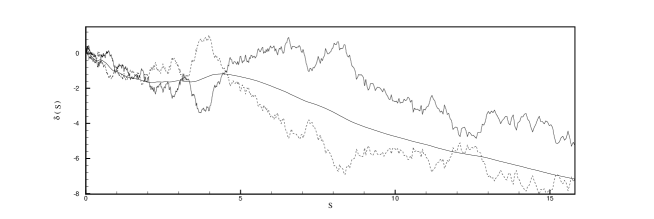
Figure 2: Role of the kernel in amplifying the walk of a tracer particle. Smooth solid, noisy-dashed and noisy-solid lines correspond to $a=1$, $a=0$ and $a=3/2$ respectively.

In Fig. 2 we show the paths of the same tracer particle for $a=1$ and for the cases $a=0$ and $a=3/2$. These paths are represented in the figure. It is clear that the path with $a=1$ is much smoother, as expected. Consequently values of $a$ control the degree of smoothness which is related to the distribution of values of $\delta(S+\mathrm{d}S)$ for given $\delta(S)$. So the values of $a$ define the correlation between various scales and, as we have shown above, a proper choice of these values results to autocorrelation functions which approximate very satisfactory the results of Eq. (4) .
Before studying mass functions we have checked the reliability of our Monte Carlo approximation by testing our results with analytical solutions. For $a=0$ or $a=3/2$ the procedure is a Wiener process and the first crossing distribution is given by the inverse Gaussian

$$f_{invG}(S)=\frac{\delta_{c}}{\sqrt{2\pi}}S^{-\frac{3}{2}}e^{-\frac{\delta^{2}_{c}}{2S}}.$$ (16)

In Fig. 3, the prediction of Eq. 16 is plotted together with the prediction of our Monte carlo approximation. The horizontal axis is $\nu=\delta_{c}(z)/\sqrt{S}$ for $z=0$. We note that this is a test with only numerical interest. The results presented in this figure are derived for $n=1000$ and $N=5\times 10^{5}$. Our results are also compared with the interesting analytical predictions of Maggiore & Riotto (2010) and Musso & Sheth (2012).
In Maggiore & Riotto (2010) the authors use a path integral approach to estimate the first crossing distributions and their results have the form of infinite series which converge slowly. Their approximation is fully consistent with the idea of the excursion set model. The resulting mass function is approximated by the formula,

Figure 3: Comparison of the results of our Monte Carlo method with the exact solution for the cases $a=0$ or $a=3/2$. The agreement is satisfactory.

$$2Sf(S)=(1-\lambda)\left(\frac{2}{\pi}\right)^{1/2}\nu e^{-\frac{1}{2}{\nu}^{2}}+\frac{\lambda}{\sqrt{2\pi}}\nu G\left(\frac{1}{2}{\nu}^{2}\right),$$ (17)

where $G(x)=\int_{x}^{\infty}t^{-1}e^{-t}\mathrm{d}t$, (see Eq. 120 in Maggiore & Riotto (2010)) .
On the other hand, in the approximation Musso & Sheth (2012) the condition of the first up-crossing is replaced by a condition of any up-crossing, while these two conditions are obviously not equivalent. Additionally, a bivariate joint distribution between $\delta$ and $v\equiv\mathrm{d}\delta/\mathrm{d}S$ is assumed, a choice which is unjustified. The mass functions is approximated by

$$2Sf(S)=Sf_{invG}R(\Gamma,\nu),$$ (18)

where

$$R(\Gamma,\nu)=\frac{1+\mathrm{erf}(\Gamma\nu\sqrt{2})}{2}+\frac{e^{-\frac{1}{2}\Gamma^{2}\nu^{2}}}{\sqrt{2\pi}\Gamma\nu},$$ (19)

where $\Gamma$ depends on the power spectrum and the kernel used to smooth the density field.

Figure 4: Comparison of the results of N-body simulations, squares, with those of analytical formulae of Eq. 17 and Eq. 18, and with our predictions. Left snapshot: squares are the results of N-body simulations. The predictions of Eq. 17 are represented by the smooth solid line while the predictions of Eq. 18 for $\Gamma=1/3$ and $\Gamma=1/2$ are represented by the dashed lines (large dashes and small dashes respectively). Right snapshot: squares are the results of N-body simulations. The results of our Monte Carlo simulations are given by the solid line.

Figure 5: Comparison of the results N-body simulations, squares, with our results. The thin solid line solid corresponds to $p=0.894$ and the thick one to $p=0.836$.

In Fig. 4, we compare the predictions of our results, derived for $a=0.796$, with those of analytical formulae of Eq. 17 and Eq. 18 with the predictions of N-body simulations at $z=0$. In both snapshots, squares are the predictions of N-body simulations of Tinker et al. (2008).

The prediction of Eq. 17 and the predictions of Eq. 18 for $\Gamma=1/3$ and for $\Gamma=1/2$ are plotted in the figure. In the right snapshot the prediction of Monte Carlo approximation. Analytical formulae of Eq.17 and Eq. 18 result to smaller numbers for heavy haloes and larger numbers for smaller haloes compared to the results of N-body simulations, while our approximation gives the correct behavior of the mass function for small haloes, $\nu\leq 1$. This is an interesting result. It shows that the excursion set model works very satisfactory for small haloes with $\nu\leq 1$. This agreement has not been reported elsewhere. On the other hand, in agreement with the analytical formulae studied above, our approximation fails to produce the correct number of heavier haloes but for $\nu\geq 1.1$ our results coincide with those of Eq. 17 and those of Eq. 19 (for $\Gamma$ =1/3). Definitely, the problem of the approximation of the correct first crossing distribution by a simple analytical formula has not been solved yet but we believe that the simplicity of the approximation formula is a secondary issue. The important issue is that of the accurate evaluation of the first crossing distributions at various scales. Our results and those of the analytical formulae of Eq. 17 and Eq. 18 indicate that the predictions of the excursion set model are, in any case, for heavy haloes far from the results of N-body simulations at least for the case of the top-hat filter and the constant barrier.
It seems possible that at large scales, additional parameters may be taken into account, as for example the ellipticity or the angular momentum of the structures. This could lead to think that the use of moving barriers as those proposed in the literature, (Bond & Myers, 1996; Del Popolo & Gambera, 1998; Sheth et al., 2001; Sheth & Tormen, 2002) is necessary. Moving barrier models try to solve the problem of the overestimation of the number of small haloes and the underestimation of the number of small haloes using a critical threshold of collapse which varies with mass ($S$). The choice of a moving barrier is based on physical arguments since larger haloes appear with the larger ellipticity and larger angular momentum. A smaller critical threshold of collapse for large haloes rearranges first crossing distributions at various scales. Studying various cases of moving barriers we found that an agreement with the predictions of N-body simulations can be achieved using a constant, lower threshold for collapse. We used a barrier of the form $\delta_{*}(z)=p\delta_{c}(z)$ where $p$ is a constant. In Fig.5 we present a comparison with the results of N-body simulations for two different values of $p$ at $z=0$. An agreement is shown. It is interesting to note the sensitivity of the distribution of heavy haloes to the values of $p$. We note that the use of a lower threshold results to an increase of the fraction $n_{cross}/N$ where $N$ is the total number of walks studied and $n_{cross}$ is the number of walks which have passed the threshold in the range $S_{min}-S_{max}$, but this increase is larger for small values of $S$ (larger haloes).

Figure 6: Comparison of our results, open squares with those of N-body simulations. The results of N-body simulations are represented by the fitting formula of Tinker et al. (2008) and are shown by the thick solid lines. Our results have been derived for $a=0.796$ and $p=0.866$.

We used $p=0.866$ as the best value. We calculated mass functions for redshifts $z=0,z=1.25$ and $z=2.5$ and we presents them in Fig. 6. Our results are plotted in the figure as are those derived from the fitting formula of Tinker et al. (2008) given in their Eq. 3 which is

Figure 7: Fractional error $[\log(MF)-\log(MF_{T})]/\log(MF_{T})$ for two redshifts $z=0$ (dotted-line) and $z=2.5$ (solid-line). $MF_{T}$ is given by the fitting formula of Tinker et al. (2008) while $MF$ represents our results.

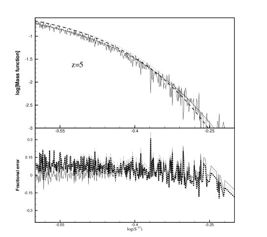
Figure 8: Upper snapshot: Mass functions at redshift $z=5$. The noisy solid line shows our results ($a=0.796,p=0.866$). The smooth solid line shows the model of Sheth et al. (2001). Dashed line represents the results of Warren et al. (2006) while dotted line shows the results of Watson et al. (2013).
Lower snapshot: Fractional errors between our results and the model of Sheth et al. (2001) , solid line, between our results and the model of Warren et al. (2006), dashed line, and between our results and the model of Watson et al. (2013), dotted line.

$$MF_{T}(\sigma,z)=A\left[\left(\frac{b}{\sigma}\right)^{a}+1\right]e^{-\frac{c}{\sigma^{2}}},$$ (20)

where $\sigma=\sqrt{S}$ and the z-dependence is given by

$$A=0.186(1+z)^{-0.14},\leavevmode\nobreak\ \leavevmode\nobreak\ a=1.47(1+z)^{-0.06},$$

$$b=2.57(1+z)^{-\alpha},\leavevmode\nobreak\ \leavevmode\nobreak\ c=1.19$$ (21)

$$\alpha=\exp\left[-\left(\frac{0.75}{\log(\Delta_{vir}/75)}\right)^{1.2}\right],$$ (22)

( See Eqs 5,6,7, and 8 in Tinker et al. (2008)). We used $\Delta_{vir}=200$.
In Fig.7 we show the fractional error, defined by $\mathrm{fr_{error}}=\frac{\log(MF)-\log(MF_{T})}{\log(MF_{T})}$ where $MF$ is the mass function derived by our model, for $z=0$ and $z=2.5$.
We note that according to Tinker et al. (2008) their model described by Eq. (20) is valid for $0\leq z\leq 2.5$. However in order to find the cause of increasing difference between our results and those of Tinker et al. (2008), shown in Fig.7, we present comparisons with some other analytical mass functions available in the literature, such that of
A. Watson et al. (2013) which is valid for $0\leq z\leq 30$. This is given by

$$MF_{Wats}=MF_{T},$$ (23)

where

$$A=0.282,\leavevmode\nobreak\ \leavevmode\nobreak\ a=2.163,\leavevmode\nobreak\ \leavevmode\nobreak\ b=1.406,\leavevmode\nobreak\ \leavevmode\nobreak\ c=1.21.$$ (24)

B. The formula of Warren et al. (2006), which is,

$$MF_{War}=0.7234(\sigma^{-1.625}+0.2538)e^{-\frac{1.1982}{\sigma^{2}}},$$ (25)

and
C. that of Sheth et al. (2001)

$$MF_{ST}=A\sqrt{\frac{2a_{s}}{\pi}}\left[1+\left(\frac{\sigma^{2}}{a_{s}\delta_{c}^{2}}\right)^{p_{s}}\right]\frac{\delta_{c}}{\sigma}e^{-\frac{a_{s}\delta_{c}^{2}}{2\sigma^{2}}},$$ (26)

where $A=0.3222,\leavevmode\nobreak\ a_{s}=0.707$ and $p_{s}=0.3$.
The comparisons for redshift $z=5$ are shown in Fig. 8. We show that the agreement remains satisfactory.
We also note that for large redshifts resolution problems appear. This is because $\delta_{c}(z)$ is an increasing function of $z$ and thus the percentage of walks which pass the barrier becomes smaller for large $z$. Large structures are more rare and the mass function appears noisy (see at the right side of Fig.8). However, it becomes difficult to check if a disagreement is due to the physical process or to the poor resolution. This difficulty rises the challenge of finding an analytical solution for the first crossing distribution of the process of Eq. 9.

In Fig. 9 we present a comparison of our results with the formula of Watson et al. (2013) and for $z=10$. These results are derived for $n=400$ and $N=5\times 10^{6}$. Resolution problems are obvious since only $4365$ from N tracer particles cross the barrier, but the agreement remains satisfactory.

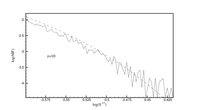
Figure 9: Mass functions at redshift $z=10$. Noisy solid line shows our results ($a=0.796,p=0.866$). The dashed line shows the model of Watson et al. (2013).

It is well known that the process of structure formation is a very complex one. It has been studied extensively in the literature and more than thirteen formulae for the mass function has been proposed for various cosmological models, various halo finding algorithms and various mass scales, see for example Watson et al. (2013) and references therein. Consequently, the probability of constructing an analytical approach that predicts the results of N-body simulations is extremely small. However, our results show that the stochastic process studied here, is not a N-body simulation, which is however able to shed more light to the physical process during the formation of structures. Since it is a process which describes accurately the correlation between scales for the realistic top-hat filter and is able to produce results close to these of N-body simulations for a constant barrier, deserves a more profound study. Any alternative approximation of first crossing distributions, resulting from the above described stochastic process, should be very interesting.

4 Acknowledgements

We acknowledge Dr. Andromachi Koufogiorgou for her kind help and J.Tinker for making available the results of their N-body simulations. ADP was supported by the Chinese Academy of Sciences and by the President’s international fellowship initiative, grant no. 2017 VMA0044.

References

- Angulo et al. (2012) Angulo, R. E., Springel, V., White, S. D. M., et al. 2012, MNRAS, 426, 2046
- Astashenok & del Popolo (2012) Astashenok, A. V. & del Popolo, A. 2012, Classical and Quantum Gravity, 29, 085014
- Bhattacharya et al. (2011) Bhattacharya, S., Heitmann, K., White, M., et al. 2011, ApJ, 732, 122
- Bond et al. (1991) Bond, J. R., Cole, S., Efstathiou, G., & Kaiser, N. 1991, ApJ, 379, 440
- Bond & Myers (1996) Bond, J. R. & Myers, S. T. 1996, ApJS, 103, 1
- Bower (1991) Bower, R. G. 1991, MNRAS, 248, 332
- Courtin et al. (2011) Courtin, J., Rasera, Y., Alimi, J.-M., et al. 2011, MNRAS, 410, 1911
- Crocce et al. (2010) Crocce, M., Fosalba, P., Castander, F. J., & Gaztañaga, E. 2010, MNRAS, 403, 1353
- Del Popolo (2007) Del Popolo, A. 2007, Astronomy Reports, 51, 169
- Del Popolo (2013) Del Popolo, A. 2013, in AIP Conf. Proc., Vol. 1548, 2–63
- Del Popolo (2014) Del Popolo, A. 2014, International Journal of Modern Physics D, 23, 30005
- Del Popolo & Gambera (1998) Del Popolo, A. & Gambera, M. 1998, A& A, 337, 96
- Del Popolo & Gambera (1999) Del Popolo, A. & Gambera, M. 1999, A& A, 344, 17
- Del Popolo & Gambera (2000) Del Popolo, A. & Gambera, M. 2000, A& A, 357, 809
- Del Popolo & Le Delliou (2017) Del Popolo, A. & Le Delliou, M. 2017, Galaxies, 5, 17
- Del Popolo & Yesilyurt (2007) Del Popolo, A. & Yesilyurt, I. S. 2007, Astronomy Reports, 51, 709
- Furlanetto et al. (2006) Furlanetto, S. R., McQuinn, M., & Hernquist, L. 2006, MNRAS, 365, 115
- Gardner (2001) Gardner, J. P. 2001, ApJ, 557, 616
- Jacobs (2010) Jacobs, K. Stochastic Processes for Physicists, Cambridge University Press
- Haiman & Loeb (2001) Haiman, Z. & Loeb, A. 2001, ApJ, 552, 459
- Hiotelis & Del Popolo (2006) Hiotelis, N. & Del Popolo, A. 2006, Ap&SS, 301, 167
- Hiotelis & del Popolo (2013) Hiotelis, N. & del Popolo, A. 2013, MNRAS, 436, 163
- Jenkins et al. (2001) Jenkins, A., Frenk, C. S., White, S. D. M., et al. 2001, MNRAS, 321, 372
- Komatsu et al. (2011) Komatsu, E., Smith, K. M., Dunkley, J., & et al. 2011, ApJS, 192, 18
- Lacey & Cole (1993) Lacey, C. & Cole, S. 1993, MNRAS, 262, 627
- Lukić et al. (2007) Lukić, Z., Heitmann, K., Habib, S., Bashinsky, S., & Ricker, P. M. 2007, ApJ, 671, 1160
- Maggiore & Riotto (2010) Maggiore, M. & Riotto, A. 2010, ApJ, 711, 907
- Malekjani et al. (2015) Malekjani, M., Naderi, T., & Pace, F. 2015, MNRAS, 453, 4148
- Musso & Sheth (2012) Musso, M. & Sheth, R. K. 2012, MNRAS, 423, L102
- Pace et al. (2014) Pace, F., Moscardini, L., Crittenden, R., Bartelmann, M., & Pettorino, V. 2014, MNRAS, 437, 547
- Peebles (1980) Peebles, P. J. E. 1980, The large-scale structure of the universe (Princeton University Press, Princeton)
- Planck Collaboration XIII (2016) Planck Collaboration XIII. 2016, A& A, 594, A13
- Press & Schechter (1974) Press, W. H. & Schechter, P. 1974, ApJ, 187, 425
- Reed et al. (2007) Reed, D. S., Bower, R., Frenk, C. S., Jenkins, A., & Theuns, T. 2007, MNRAS, 374, 2
- Sheth et al. (2001) Sheth, R. K., Mo, H. J., & Tormen, G. 2001, MNRAS, 323, 1
- Sheth & Tormen (1999) Sheth, R. K. & Tormen, G. 1999, MNRAS, 308, 119
- Sheth & Tormen (2002) Sheth, R. K. & Tormen, G. 2002, MNRAS, 329, 61
- Smith et al. (1998) Smith, C. C., Klypin, A., Gross, M. A. K., Primack, J. R., & Holtzman, J. 1998, MNRAS, 297, 910
- Tinker et al. (2008) Tinker, J., Kravtsov, A. V., Klypin, A., et al. 2008, ApJ, 688, 709
- Warren et al. (2006) Warren, M. S., Abazajian, K., Holz, D. E., & Teodoro, L. 2006, ApJ, 646, 881
- Watson et al. (2013) Watson, W. A., Iliev, I. T., D’Aloisio, A., et al. 2013, MNRAS, 433, 1230
- Weinberg (1989) Weinberg, S. 1989, Reviews of Modern Physics, 61, 1
- White (2002) White, M. 2002, ApJS, 143, 241