Properties of dirty two-bands superconductors with repulsive interband interaction:
normal modes, length scales, vortices and magnetic response

Abstract

Disorder in two-band superconductors with repulsive interband interaction induces a frustrated competition between the phase-locking preferences of the various potential and kinetic terms. This frustrated interaction can result in the formation of an $s+is$ superconducting state, that breaks the time-reversal symmetry. In this paper we study the normal modes and their associated coherence lengths in such materials. We especially focus on the consequences of the soft modes stemming from the frustration and time-reversal-symmetry breakdown. We find that two-bands superconductors with such impurity-induced frustrated interactions display a rich spectrum of physical properties that are absent in their clean counterparts. It features a mixing of Leggett’s and Anderson-Higgs modes, and a soft mode with diverging coherence length at the impurity-induced second order phase transition from $s_{\pm}/s_{++}$ states to the $s+is$ state. Such a soft mode generically results in long-range attractive intervortex forces that can trigger the formation of vortex clusters. We find that, if such clusters are formed, their size and internal flux density have a characteristic temperature dependence that could be probed in muon-spin-rotation experiments. We also comment on the appearance of spontaneous magnetic fields due to spatially varying impurities.

I Introduction

The discovery of iron-based superconductors motivated research on two-band superconductors where the pairing between electrons is produced by interband electron-electron repulsion Mazin et al. (2008); Chubukov et al. (2008); Hirschfeld et al. (2011). Such systems tend to form a state with two $s$-wave gaps $\Delta_{i}=|\Delta_{i}|\text{e}^{i\theta_{i}}$ (with $i=1,2$), for which the relative phase differs by $\pi$ (that is, $\theta_{2}=\theta_{1}+\pi$). This superconducting state with a sign change between the gap functions is called $s_{\pm}$, in contrast to the more commonly studied $s_{++}$ state, which has a zero relative phase ($\theta_{1}=\theta_{2}$). The $s_{\pm}$ superconducting state behaves non trivially when disorder is added. It is indeed known that, under certain conditions, impurities induce a crossover from the $s_{\pm}$ to the $s_{++}$ state. At temperatures sufficiently close to the critical temperature $T_{c}$, the transition from the $s_{\pm}$ to the $s_{++}$ state is realized as a direct crossover, with little thermodynamic features, where one of the gap function is completely suppressed Efremov et al. (2011). It was nonetheless recently demonstrated that, due to competing kinetic and potential terms, inhomogeneous states such as vortices or screening currents become structurally nontrivial in the vicinity of that crossover Garaud et al. (2017, 2018).

At lower temperatures, the impurity-induced transition to the $s_{++}$ state occurs via an intermediate state where the inter-component relative phase is different from $0$ and $\pi$ Bobkov and Bobkova (2011); Stanev and Koshelev (2014). This state is called $s+is$ state. It spontaneously breaks the time-reversal symmetry, and is separated from the standard $s_{\pm}/s_{++}$ states by a second-order phase transition (at mean-field level). However quantitative calculations of the phase diagram demonstrated Silaev et al. (2017) that the impurity induced $s+is$ state occupies a vanishingly small region of the phase diagram and is unlikely to be observable directly. Note that this statement applies only to weak-coupling mean-field theory of dirty two-band system. This behavior is drastically different from that found in systems with three or more interacting bands, where the $s+is$ state appears as a result of the frustrated interband repulsive pairing Ng and Nagaosa (2009); Stanev and Tešanović (2010); Carlström et al. (2011a); Maiti and Chubukov (2013); Böker et al. (2017).

In this work we demonstrate that, even if the $s+is$ state occupies a very small region, its mere presence on the phase diagram can still have important consequences. Indeed, as previously stated the $s+is$ state spontaneously breaks the time-reversal symmetry. Thus, in addition to the usual $\mathrm{U}(1)$ symmetry, the $s+is$ state also breaks the discrete $\mathbb{Z}_{2}$ symmetry associated with the time-reversal operations. In other words, since the relative phase between the gaps is neither $0$ nor $\pi$, complex conjugation leads to another state that cannot be rotated back to the initial state by $\mathrm{U}(1)$ transformation. Because $s_{\pm}/s_{++}$ are different on symmetry grounds from the $s+is$ state, at the mean-field level the phase transition is second order. This implies that there is a divergent coherence length inside the superconducting state on both sides of the $s+is$ domain Silaev et al. (2017).

Here we demonstrate that the emerging soft normal mode with divergent coherence length is not only associated with the relative phase (Leggett’s mode), but also with the amplitude (Higgs modes). This leads to the situation that $s_{\pm}/s_{++}$ states adjacent to the $s+is$ domain should acquire unconventional properties associated with the static and dynamic fluctuations, the nature of topological excitations, and the magnetic response to an external applied field. Therefore dirty two-band superconductors with a repulsive interband interaction have a much more complex behavior than the well studied standard $s_{++}$ state in clean systems where, by contrast, the existence of soft modes away from superconducting phase transition, requires only weak interband coupling Silaev and Babaev (2011).

The paper is organized as follows. In section II, starting from the microscopic Usadel theory of dirty two-band superconductors, we provide a detailed derivation of the corresponding two-band Ginzburg-Landau model, and discuss the essential properties of the phase diagram. Next, section III is devoted to the complete analysis of the linearized theory. This provides the framework to describe the behavior of the coherence lengths and their associated normal modes, across the different phases of the phase diagram. The derived perturbation operator can also be used to determine the upper critical fields of such dirty two-band superconductors. This is discussed separately in an appendix. The perturbation operator features a divergent length scale in the vicinity of the second order phase transition to the $s+is$ phase. The existence of such a soft mode can result in long-range attractive intervortex forces. In section IV we investigate this property beyond the linear regime regime, and demonstrate that vortex clusters can form in the vicinity of the $s+is$ phase, and that they feature specific temperature dependent properties.

Readers who are not interested in technical details of the analysis of normal models but are interested in properties of vortex states and their possible experimental manifestations can, after Sec. II, directly proceed to Sec. IV.

II Ginzburg-Landau model derived from the Usadel equations

We investigate the properties of the superconducting states, their characteristic length scales and vortex structures within a weak-coupling model of two-band superconductors with high concentration of impurities. Such material can be described by a system of two Usadel equations coupled together by interband impurity scattering terms Gurevich (2003):

$$\omega_{n}f_{i} =\frac{D_{i}}{2}\big{(}g_{i}{\bm{\Pi}}^{2}f_{i}-f_{i}\nabla^{2}g_{i}\big{)}+\Delta_{i}g_{i}$$

$$\leavevmode\nobreak\ \leavevmode\nobreak\ \leavevmode\nobreak\ +\sum_{j\neq i}\gamma_{ij}(g_{i}f_{j}-g_{j}f_{i})\,,$$ (1)

where $\omega_{n}=(2n+1)\pi T$, with $n\in\mathbb{Z}$, are the fermionic Matsubara frequencies. $T$ stands for the temperature, $D_{i}$ are the electron diffusivities, and $\gamma_{ij}$ are the interband scattering rates.

The quasi-classical propagators $f_{i}$ and $g_{i}$, which are, respectively, the anomalous and normal Green’s functions in each band, obey the normalization condition $|f_{i}|^{2}+g_{i}^{2}=1$. The two components $\Delta_{j}=|\Delta_{j}|e^{i\theta_{j}}$ of the order parameter are determined by the self-consistency equations

$$\Delta_{i}=2\pi T\sum_{n=0}^{N_{d}}\sum_{j}\lambda_{ij}f_{j}(\omega_{n}),$$ (2)

for the Green’s functions that satisfy the Usadel equation Eq. (II). Here, $N_{d}=\Omega_{d}/(2\pi T)$ is the summation cut-off at the Debye frequency $\Omega_{d}$. In the self-consistency equation (2), the diagonal elements $\lambda_{ii}$ of the coupling matrix $\hat{\lambda}$ describe the intraband pairing, while the interband interaction is determined by the off-diagonal terms $\lambda_{ij}$ ($j\neq i$). The interband coupling parameters and impurity scattering amplitudes satisfy the symmetry relation Gurevich (2003):

$$\lambda_{ij}=-\lambda_{J}/n_{i}\leavevmode\nobreak\ \leavevmode\nobreak\ \text{and}\leavevmode\nobreak\ \leavevmode\nobreak\ \gamma_{ij}=\Gamma n_{j}\,,$$ (3)

where $\lambda_{J}$ and $\Gamma>0$. The impurity scattering rate is given in units of $T_{c}$, $n_{i}=N_{i}/(N_{1}+N_{2})$ are the relative densities of states, and $N_{1,2}$ are the partial densities of states in the two-bands.

In general, the $s_{\pm}$ state is not favored by the impurity scattering, which tends to average out the order parameter over the whole Fermi surface, suppressing the critical temperature. Still, provided the interband pairing interaction is weak, superconductivity can be transformed into a $s_{++}$ state and survive even in the limit $\Gamma\gg T_{c0}$, characterized by the critical temperature $T_{c\infty}$ which reads as Stanev and Koshelev (2014); Hirschfeld et al. (2011):

$$\ln(T_{c0}/T_{c\infty})=N_{1}(w_{11}+w_{12})+N_{2}(w_{22}+w_{21})\,,$$ (4)

where $T_{c0}$ is the critical temperature in the absence of interband scattering, $\hat{w}=\hat{\Lambda}^{-1}-z^{-1}\hat{I}$ and $z$ is the maximal eigenvalue of the coupling matrix $\hat{\Lambda}$ with the elements $\lambda_{kk^{\prime}}$. In order to avoid a drastic suppression of the critical temperature in the $s_{++}$ state, according to Eq. (4), the interband interaction $\lambda_{J}$ should be sufficiently weak. To derive a criterion, note that $N_{1}w_{11}+N_{2}w_{22}>0$, so that the r.h.s. of the Eq. (4) is larger than $N_{1}w_{12}+N_{2}w_{21}=\lambda_{J}/(\lambda_{11}\lambda_{22})$. Therefore, in order to have a $T_{c\infty}$ which is not much smaller than $T_{c0}$, we require the following condition $\lambda_{J}/(\lambda_{11}\lambda_{22})<1$ to be satisfied.

II.1 Ginzburg-Landau expansion

The two-band Ginzburg-Landau (GL) expansion is an expansion in two small gaps and small gradients [not to be confused with a single-parameter expansion $\tau=(1-T/T_{c})$]. A detailed discussion of the formal validity of multiband expansions in the context of clean system can be found in Silaev and Babaev (2012). It was demonstrated in Ref. Silaev et al., 2017 that for dirty systems, in the region of its applicability, the Ginzburg-Landau model gives a phase diagram that matches that of the microscopic Usadel theory. Here, we provide the full derivation of the GL expansion including gradient terms. In the case of a dirty system, by inverting the self-consistency equation (2), it is found that:

$$2\pi T\sum_{n=0}^{N_{d}}f_{i}(\omega_{n})=\frac{\lambda_{jj}\Delta_{k}-\lambda_{ij}\Delta_{j}}{\mathrm{det}\hat{\lambda}}\leavevmode\nobreak\ \leavevmode\nobreak\ \leavevmode\nobreak\ \leavevmode\nobreak\ \text{and}\leavevmode\nobreak\ j\neq i\,.$$ (5)

and defining the expansion for the $f_{i}$ from the Usadel equation (II). In the first approximation we put $g^{(0)}_{i}=1$ (at $\omega_{n}>0$) and thus find

$$f^{(1)}_{i}=\frac{\gamma_{ij}\Delta_{j}+(\omega_{n}+\gamma_{ji})\Delta_{i}}{\omega_{n}(\omega_{n}+\gamma_{ij}+\gamma_{ji})}\leavevmode\nobreak\ \leavevmode\nobreak\ \leavevmode\nobreak\ \leavevmode\nobreak\ \text{and}\leavevmode\nobreak\ j\neq i\,.$$ (6)

The corrections $f^{(3)}_{i}$ from the non-linear terms in Eq. (II) are found by neglecting the gradients from which follows the general relation

$$f_{i}=\frac{\Delta_{i}(\omega_{n}+\gamma_{ji}g_{i})+\gamma_{ij}\Delta_{j}g_{j}}{\omega_{n}(\omega_{n}+\gamma_{ij}g_{j}+\gamma_{ji}g_{i})}g_{i}\,.$$ (7)

Then, when taking into account the corrections, $g_{i}=1-|f_{i}^{(1)}|^{2}/2$, and this yields

$$f^{(3)}_{i}= -\frac{|f^{(1)}_{i}|^{2}\Delta_{i}\left[\left(\omega_{n}+\gamma_{ji}\right)^{2}+\gamma_{ij}(\omega_{n}+2\gamma_{ji})\right]}{2\omega_{n}(\omega_{n}+\gamma_{ij}+\gamma_{ji})^{2}}$$

$$-\frac{|f^{(1)}_{i}|^{2}\Delta_{j}(\omega_{n}+\gamma_{ij})\gamma_{ij}}{2\omega_{n}(\omega_{n}+\gamma_{ij}+\gamma_{ji})^{2}}$$

$$+\frac{|f^{(1)}_{j}|^{2}\gamma_{ij}(\omega_{n}+\gamma_{ji})(\Delta_{i}-\Delta_{j})}{2\omega_{n}(\omega_{n}+\gamma_{ij}+\gamma_{ji})^{2}}\,.$$ (8)

Finally, combining the equations (7) and (II.1) yields the non-linear terms in the Ginzburg-Landau expansion. The corrections $f^{(g)}_{i}$ from the gradient terms are obtained by linearizing Usadel equation (II), with respect to the corrections $f^{(g)}_{i}$. This yields

$$f^{(g)}_{i}= \frac{D_{i}(\omega_{n}+\gamma_{ji})^{2}+D_{j}\gamma_{ij}\gamma_{ji}}{2\omega_{n}^{2}(\omega_{n}+\gamma_{ij}+\gamma_{ji})^{2}}{\bm{\Pi}}^{2}\Delta_{i}$$

$$+\frac{\gamma_{ij}\left[D_{i}(\omega_{n}+\gamma_{ji})+D_{j}(\omega_{n}+\gamma_{ij})\right]}{2\omega_{n}^{2}(\omega_{n}+\gamma_{ij}+\gamma_{ji})^{2}}{\bm{\Pi}}^{2}\Delta_{j}\,.$$ (9)

Finally, the Ginzburg-Landau functional reads as

$$\frac{\mathcal{F}}{\mathcal{F}_{0}}= \sum_{j=1}^{2}\Big{\{}\frac{k_{jj}}{2}\left|{\bm{\Pi}}\Delta_{j}\right|^{2}+a_{jj}|\Delta_{j}|^{2}+\frac{b_{jj}}{2}|\Delta_{j}|^{4}\Big{\}}$$ (10a)

$$+\frac{k_{12}}{2}\Big{(}({\bm{\Pi}}\Delta_{1})^{*}{\bm{\Pi}}\Delta_{2}+({\bm{\Pi}}\Delta_{2})^{*}{\bm{\Pi}}\Delta_{1}\Big{)}$$ (10b)

$$+2\left(a_{12}+c_{11}|\Delta_{1}|^{2}+c_{22}|\Delta_{2}|^{2}\right)\mathrm{Re}\big{(}\Delta_{1}^{*}\Delta_{2}\big{)}$$ (10c)

$$+\left(b_{12}+c_{12}\cos 2\theta_{12}\right)|\Delta_{1}|^{2}|\Delta_{2}|^{2}+\frac{{\bm{B}}^{2}}{2}\,.$$ (10d)

Here, $\theta_{12}=\theta_{2}-\theta_{1}$ stands for the relative phase between the complex fields $\Delta_{j}=|\Delta_{j}|e^{i\theta_{j}}$ that represent the superconducting gaps in the different bands. The two gaps in the different bands are electromagnetically coupled by the vector potential ${\bm{A}}$ of the magnetic field ${\bm{B}}=\bm{\nabla}\times{\bm{A}}$, through the gauge derivative ${\bm{\Pi}}\equiv{\bm{\nabla}}+iq{\bm{A}}$. The coefficients of the Ginzburg-Landau functional $a_{ij}$, $b_{ij}$, $c_{ij}$ and $k_{ij}$ can be calculated from a given set of input microscopic parameters $\lambda_{ij}$, $D_{i}$, $T$ and $\Gamma$ of the microscopic self-consistency equation. Their explicit formulas are listed in Appendix A.

As can be seen in Eq. (II.1), the coefficients of the gradient terms depend on both electronic diffusivity coefficients $D_{1}$ and $D_{2}$. Clearly, the parameter space can be reduced by absorbing one of the electronic diffusivity coefficient in the gradient term. Without any loss of generality, we choose $D_{1}$ to be the largest diffusivity coefficient ($D_{1}>D_{2}$). Thus, in the dimensionless units, the coefficients of the gradient term depend only on the ratio of diffusivities, or relative diffusion constant $r_{d}=D_{2}/D_{1}<1$. The free energy (10) is expressed in terms of dimensionless quantities, so the coupling constant $q$ should not be confused with $2\pi/\Phi_{0}$. In such units, the coupling constant $q$ instead parametrizes the penetration depth of the magnetic field (see units detail below). The dimensionless units are defined as:

$${\bm{\nabla}}=\xi_{0}\tilde{{\bm{\nabla}}}\,,\leavevmode\nobreak\ \leavevmode\nobreak\ {\bm{A}}=\tilde{{\bm{A}}}/B_{0}\xi_{0}\,,\leavevmode\nobreak\ \leavevmode\nobreak\ \Delta=\tilde{\Delta}/T_{c}\,,$$ (11)

where the variables with tilde are the dimensionful quantities. Therefore $\xi_{0}=\sqrt{D_{1}/T_{c}}$ is the new unit of the length, and $B_{0}=T_{c}\sqrt{4\pi N_{1}}$ the unit of the magnetic field (here $N_{1}$ is the density of states in the first band). The free energy is then scaled by ${\mathcal{F}_{0}}=B_{0}^{2}/4\pi$, while the electromagnetic coupling constant becomes $q=2\pi B_{0}\xi_{0}^{2}/\Phi_{0}$.

In these new units, the London penetration length $\lambda_{L}$ is given by $\lambda^{-2}_{L}=q^{2}(k_{ii}\Delta_{i0}^{2}+2k_{12}\Delta_{10}\Delta_{20})$, where $\Delta_{i0}$ is the bulk value of the dimensionless gap. Correspondingly the gauge field coupling constant is $q=\lambda_{L}(k_{ii}\Delta_{i0}^{2}+2k_{12}\Delta_{10}\Delta_{20})^{-1/2}$. Eventually, for a given set of input microscopic parameters, $\lambda_{ij}$, $\Gamma$, $r_{d}$, and $T$ close to $T_{c}$, we can reconstruct the coefficients and investigate the ground-state properties of the GL theory by minimizing the free energy (10) with respect to $|\Delta_{j}|$ and $\theta_{12}$.

II.2 Phase diagrams

The mean-field phase diagram of the dirty two-band superconductors was calculated in Silaev et al. (2017), using both Usadel and Ginzburg-Landau formalisms. It was demonstrated there, that the phase diagrams are quantitatively similar within the range of validity of GL expansion. Here we briefly outline the structure of the diagram within the Ginzburg-Landau model. Knowing the coefficients (see details in Appendix A) of the microscopically derived Ginzburg-Landau functional (10), allows to investigate the ground-state properties of dirty two-bands superconductors by minimizing the free energy (10) with respect to $|\Delta_{j}|$ and $\theta_{12}$.

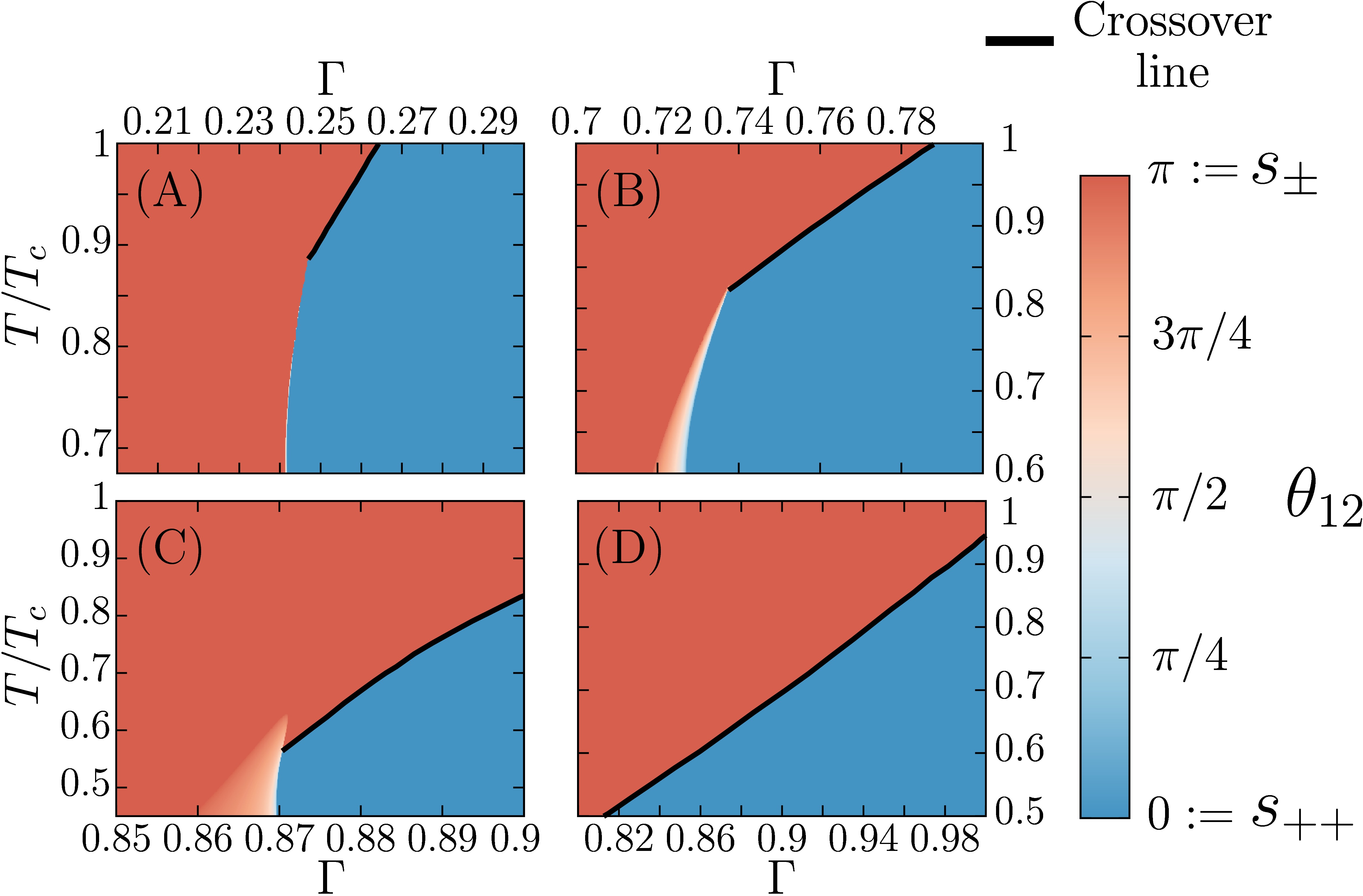
Figure 1: Phase diagrams of the Ginzburg-Landau free energy (10) describing two-band superconductors with interband impurity scattering. These show the values of the lowest-energy state relative phase $\theta_{12}=\theta_{2}-\theta_{1}$ between the components of the order parameter, as function of temperature and interband scattering $\Gamma$. The different panels correspond to different values of the coupling matrix $\hat{\lambda}$. Panels (A), (B), and (C) respectivelly correspond to nearly degenerate bands with $\lambda_{11}=0.29$ and $\lambda_{22}=0.3$ with weak $\lambda_{12}=\lambda_{21}=-0.01$, intermediate $\lambda_{12}=\lambda_{21}=-0.05$ and strong $\lambda_{12}=\lambda_{21}=-0.1$ repulsive interband pairing interaction. The last panel (D) describes the case of intermediate band disparity $\lambda_{11}=0.25$ and $\lambda_{22}=0.3$ with intermediate $\lambda_{12}=\lambda_{21}=-0.05$ repulsive interband pairing interaction. The solid black line shows the zero of $\Delta_{2}$, that is the crossover between $s_{\pm}$ and $s_{++}$ states. In panels (A), (B) and (C), the crossover line is attached to a dome of time-reversal symmetry breaking $s+is$ state. In the panel (D), the crossover line does not connect to an $s+is$ state.

The phase diagrams are constructed in the plane of parameters $\Gamma,T$ of a two-band superconductor with interband impurity scattering. For that purpose, we numerically minimize the free energy (10) using a nonlinear conjugate gradient algorithm. The results displayed in Fig. 1 demonstrate the role of impurities on the ground state properties, for various representative cases. Namely nearly degenerate bands with weak (A), intermediate (B) and strong (C) repulsive interband pairing interactions (as compared to the intraband couplings). Also, we consider the case of intermediate band disparity with intermediate interband coupling (D).

Those diagrams illustrate the now well understood fact that, in two-band superconductors, disorder may induce a transition from the $s_{\pm}$ state (the red regions with $\theta_{12}=\pi$ in Fig. 1) to the $s_{++}$ state (the blue regions with $\theta_{12}=0$ in Fig. 1) Efremov et al. (2011); Bobkov and Bobkova (2011); Stanev and Koshelev (2014); Silaev et al. (2017). The transition can occur in two qualitatively different ways. Either via a direct crossover (denoted by a solid black line) when one of the superconducting gap vanishes as a function of impurity concentration Efremov et al. (2011), or via the intermediate complex $s+is$ state that break time-reversal symmetry with $\theta_{12}\neq 0,\pi$. The crossover occurs without additional symmetry breaking while the transition via an $s+is$ state spontaneously breaks the time-reversal symmetry, and both $s_{\pm}/s+is$ and $s_{++}/s+is$ transitions lines are of the second order, at the mean-field level Silaev et al. (2017). As was mentioned in the Introduction, the existence of the second-order phase transition on the phase diagram dictates that there is softening of one of the normal modes near that transition. This softening has a number of possible physical consequences. That motivates the study performed in the next section, where we consider the normal modes of this system.

III Linear analysis: normal modes and coherence lengths

An analysis of the perturbation operator around classical solutions such as the ground state, or the normal state provides important informations such as the length scales of the theory, the zero modes or the upper critical field. To facilitate this analysis, we find it convenient here to rewrite the Ginzburg-Landau free energy (10) in terms of a new rotated field basis (linear combination) that eliminates the mixed gradient terms.

III.1 Elimination of mixed gradient terms

Because it features mixed gradient terms, the original basis for the superconducting degrees of freedom is quite inconvenient to work with. This is why it is worth rewriting the model using a linear combination of the components of the order parameter that diagonalizes the kinetic terms:

$$\psi_{1}=\sqrt{k_{11}}\Delta_{1}+\sqrt{k_{22}}\Delta_{2}\,,\leavevmode\nobreak\ \leavevmode\nobreak\ \psi_{2}=\sqrt{k_{11}}\Delta_{1}-\sqrt{k_{22}}\Delta_{2}\,.$$ (12)

Within this new basis, we refer to as rotated basis, the kinetic term has a much simpler form. The potential, on the other hand becomes more involved. Yet it is a convenient basis to deal with, for the determination of the physical length scales as well as describing various unusual properties. In the new rotated field basis, the free energy reads as

$$\mathcal{F}=\sum_{j=1}^{2}\Big{\{}\frac{\kappa_{j}}{2}\left|{\bm{\Pi}}\psi_{j}\right|^{2}+\alpha_{jj}|\psi_{j}|^{2}+\frac{\beta_{jj}}{2}|\psi_{j}|^{4}\Big{\}}$$ (13a)

$$+2\left(\alpha_{12}+\gamma_{11}|\psi_{1}|^{2}|+\gamma_{22}\psi_{2}|^{2}\right)|\psi_{1}||\psi_{2}|\cos\varphi_{12}$$ (13b)

$$+\left(\beta_{12}+\gamma_{12}\cos 2\varphi_{12}\right)|\psi_{1}|^{2}|\psi_{2}|^{2}+\frac{{\bm{B}}^{2}}{2}\,,$$ (13c)

with the rotated superconducting degrees of freedom $\psi_{j}=|\psi_{j}|\text{e}^{i\varphi_{j}}$, and $\varphi_{12}=\varphi_{2}-\varphi_{1}$, and the coefficients for the kinetic term are now

$$\kappa_{1}=\frac{\sqrt{k_{11}k_{22}}+k_{12}}{2\sqrt{k_{11}k_{22}}}\leavevmode\nobreak\ \leavevmode\nobreak\ \leavevmode\nobreak\ \leavevmode\nobreak\ \text{and}\leavevmode\nobreak\ \leavevmode\nobreak\ \leavevmode\nobreak\ \leavevmode\nobreak\ \kappa_{2}=\frac{\sqrt{k_{11}k_{22}}-k_{12}}{2\sqrt{k_{11}k_{22}}}\,.$$ (14)

Upon some algebraic manipulations, all coefficients $\alpha_{ij}$, $\beta_{ij}$, $\gamma_{ij}$ of the potential, are expressed in terms of the coefficients $a_{ij}$, $b_{ij}$, $c_{ij}$ and $k_{ij}$ of the original Ginzburg-Landau functional (10). Detailed expressions of new parameters can be found in Appendix B. Within the framework of new rotated variables (12), the Ginzburg-Landau equations have no mixed-gradients and read as

$${\bm{\Pi}}^{2}\psi_{j}=2\frac{\partial V}{\partial\psi_{j}^{*}}\,.$$ (15)

The variation of the free energy (13) with respect to the vector potential ${\bm{A}}$, determines Ampère’s equation ${\bm{\nabla}}\times{\bm{B}}+{\bm{J}}=0$. There, the total current is the superposition of the partial currents (${\bm{J}}=\sum_{i}{\bm{J}}^{(i)}$) that reads as

$${\bm{J}}^{(i)}=q\kappa_{i}\mathrm{Im}\big{(}\psi_{i}^{*}{\bm{\Pi}}\psi_{i}\big{)}\,.$$ (16)

The reparametrization (12) simplifies drastically the Ginzburg-Landau equations as there is no more coupling of the components through mixed gradients. However, this comes with the price of more complicated potential terms. This is actually a minor issue, since the ground state within the rotated basis, can easily be determined from the one in the original field basis according to the formulas

$$|\psi_{1}|^{2} =k_{11}|\Delta_{1}|^{2}+k_{22}|\Delta_{2}|^{2}+2\sqrt{k_{11}k_{22}}|\Delta_{1}||\Delta_{2}|\cos\theta_{12}\,,$$

$$|\psi_{2}|^{2} =k_{11}|\Delta_{1}|^{2}+k_{22}|\Delta_{2}|^{2}-2\sqrt{k_{11}k_{22}}|\Delta_{1}||\Delta_{2}|\cos\theta_{12}\,,$$

$$\varphi_{12} =\tan^{-1}\left(\frac{-2\sqrt{k_{11}k_{22}}|\Delta_{1}||\Delta_{2}|\sin\theta_{12}}{k_{11}|\Delta_{1}|^{2}-k_{22}|\Delta_{2}|^{2}}\right)\,.$$ (17)

To understand the role of excitations, as well as the fundamental length scales of the Ginzburg-Landau free energy (13), it can be rewritten in terms of gauge invariant quantities (i.e. in terms of charged and neutral modes (see a general discussion in the context of a simpler model in Babaev et al. (2002); Babaev (2002)) by expanding the kinetic term in (13a) and using (16):

$$\mathcal{F}=\frac{1}{2}({\bm{\nabla}}\times{\bm{A}})^{2}+\frac{{\bm{J}}^{2}}{2q^{2}\varrho^{2}}+\sum_{a}\frac{\kappa_{a}}{2}({\bm{\nabla}}|\psi_{a}|)^{2}$$

$$+\frac{\kappa_{1}\kappa_{2}|\psi_{1}|^{2}|\psi_{2}|^{2}}{2\varrho^{2}}({\bm{\nabla}}\varphi_{12})^{2}+V(|\psi_{1}|,|\psi_{2}|,\varphi_{12})\,.$$ (18)

Here again $\varphi_{12}=\varphi_{2}-\varphi_{1}$ stands for the relative phase between the condensates, and $\varrho^{2}=\sum_{i}\kappa_{i}|\psi_{i}|^{2}$. For this rewriting, we used the supercurrent defined from the Ampère’s equation ${\bm{\nabla}}\times{\bm{B}}+{\bm{J}}=0$, that reads

$${\bm{J}}/q=q\varrho^{2}{\bm{A}}+\sum_{i}\kappa_{i}|\psi_{i}|^{2}{\bm{\nabla}}\varphi_{a}\,.$$ (19)

As discussed below, due to absence of mixed gradient terms, this formulation allows an easier calculation of the length scales and a better interpretation of the corresponding normal modes.

III.2 Coherence lengths and perturbation operator

The length scales that characterize matter fields are called coherence lengths. Fundamentally the coherence length $\xi$ associated to a field $\Psi({r})$ is defined through the exponent that characterizes how, from a small perturbation, the field recovers its ground state value $\bar{\Psi}$ (see, e.g., Tinkham (1995); Plischke and Bergersen (1989); Svistunov et al. (2015)). That is, from a perturbation $\Psi({r})\approx\bar{\Psi}$, the field recovers according to the asymptotic behavior

$$\Psi({r})-\bar{\Psi}\propto e^{-\frac{r}{\xi}}\ \ \ \ (r\gg\xi)\,.$$ (20)

Note that, typically in the context of superconductivity the definition of the coherence length has an extra $\sqrt{2}$ factor Tinkham (1995), while this factor is absorbed into the definition of $\xi$ in other contexts. Here we follow the more general definition and absorb this factor into $\xi$. Note also that for the simplest Ginzburg-Landau model the coherence length is occasionally indirectly assessed, for example through overall vortex core size or from the slope of the order parameter near the center of the vortex core. Only in some special cases all these estimates give consistent results. For example, even in the simplest single-component $s$-wave superconductors, away from $T_{c}$ all these definitions give inconsistent results Gygi and Schlüter (1991). In a multi-component systems, the length scales physics is more complicated so they should not be a priori expected to be easily assessable from such quantities as the order parameter slope near the origin. Another consequence of intercomponent interactions, is that it cannot be expected that independent coherence lengths are associated with single fields $\Delta_{j}$. Instead one can expect to find linear combinations of the complex fields that recover from a perturbation with different exponential laws (20) and therefore are characterised by different coherence lengths. In general, in multi-component GL models, determination of the various coherence lengths cannot be done analytically, except in the cases of weak interband interaction, where the intercomponent interactions can be addressed perturbatively Carlström et al. (2011b). Thus generic determination of the coherence lengths has to be carried out numerically.

To determine the coherence lengths one thus consider the small perturbations in all relevant field degrees of freedom around a physical solution, and linearize the theory around that solution. Such a physical solution is for example the ground-state, the normal state, etc. The eigenvalue spectrum of the infinitesimal perturbation operator are the (squared) masses of the normal modes, and the coherence lengths are defined as the inverse masses. Thus, the eigenspectrum of the obtained (linear) differential operator determines the masses of the normal modes and consequently their corresponding length scales. In the single-component limit that corresponds to the standard calculation Tinkham (1995). By contrast, the model we consider here has four degrees of freedom associated with the matter fields: two moduli and two phases of the complex fields.

If one neglect the coupling to vector potential then the sum of the phases forms a mode with zero mass (the Goldstone mode), since it is associated with a broken $\mathrm{U}(1)$ symmetry. When coupling to the vector potential is included this mode becomes massive via the London-Anderson-Higgs mechanism. The inverse of that mass is the London’s magnetic field penetration length. For the simplest two-band $s_{++}$ material the phase difference constitute another massive mode that, in a dynamical context, is called the Leggett’s mode Leggett (1966). In a static case the length scale associated with this mode (i.e. the length scale at which the phase difference recovers from a perturbation) is also called Josephson length. However it was discussed in clean three-band superconductors, that when time-reversal symmetry is broken, there is no Leggett-type (phase-only) mode, and instead the phase difference mode is hybridized (i.e. mixed) with the density (Higgs) modes Carlström et al. (2011a); Maiti and Chubukov (2013); Stanev (2012); Marciani et al. (2013). Below, we find that in impurities-induced $s+is$ case the modes are mixed as well. As dictated by the theory of the mean-field second order phase transitions, mass of one of the modes should go to zero at the superconducting phase transition (indeed at this transition $\mathbb{Z}_{2}$ symmetry is broken and thus there is divergence of one of the coherence lengths, while other length scales should remain finite). In Ref. Silaev et al., 2017 it was demonstrated that the transition to the $s+is$ state from $s_{++}$ or $s_{\pm}$ state is second order at the mean-field level. This dictates that there should be a divergent coherence length at that transition as well.

The perturbation theory is constructed as follows. The fields are expanded in series of a small parameter $\epsilon$: $\psi_{i}=\sum_{a}\epsilon^{a}\psi_{i}^{(a)}$ and collected order by order in the functional. The zeroth order is the original functional, while the first order is identically zero provided the leading order in the series expansion satisfies the equations of motion. Because we expand near a classical state (for example the ground state), physically relevant correction thus appear at the order $\epsilon^{2}$ of the expanded Ginzburg-Landau functional. The length scale analysis is done by applying the previously discussed perturbative theory to the case where the leading order is the ground-state.

We choose the following expansion in small perturbations around the ground state

$$|\psi_{i}|=u_{i}+\frac{\epsilon f_{i}}{\sqrt{\kappa_{i}}}\,,\leavevmode\nobreak\ \leavevmode\nobreak\ \varphi_{12}={\bar{\varphi}}+\epsilon\sqrt{\frac{\kappa_{1}u_{1}^{2}+\kappa_{2}u_{2}^{2}}{\kappa_{1}\kappa_{2}u_{1}^{2}u_{2}^{2}}}\phi\,.$$ (21)

where $u_{i}$ and ${\bar{\varphi}}$ denote the ground state while $f_{i}$ and $\phi$, stand for the perturbations. $\epsilon$ is the arbitrarily small parameter of the series expansion. Collecting the perturbations in a single vector $\Upsilon=(f_{1},f_{2},\phi)^{T}$, the term which is second order in $\epsilon$ in the Ginzburg-Landau functional (III.1) reads as:

$$\frac{1}{2}\Upsilon^{T}\left({\bm{\nabla}}^{2}+{\cal M}^{2}\right)\Upsilon\,,$$ (22)

where the diagonal entries of the (squared) mass matrix are:

$${\cal M}^{2}_{f_{i}f_{i}} =\frac{2}{\kappa_{i}}\Big{(}\alpha_{ii}+3\beta_{ii}u_{i}^{2}+(\beta_{12}+\gamma_{12}\cos 2{\bar{\varphi}})u_{j}^{2}$$

$$\leavevmode\nobreak\ \leavevmode\nobreak\ \leavevmode\nobreak\ \leavevmode\nobreak\ \leavevmode\nobreak\ +6\gamma_{ii}u_{1}u_{2}\cos{\bar{\varphi}}\Big{)}$$ (23a)

$${\cal M}^{2}_{\phi\phi} =-\frac{\kappa_{1}u_{1}^{2}+\kappa_{2}u_{2}^{2}}{\kappa_{1}\kappa_{2}u_{1}^{2}u_{2}^{2}}\Big{(}4\gamma_{12}u_{1}^{2}u_{2}^{2}\cos 2{\bar{\varphi}}$$

$$\leavevmode\nobreak\ \leavevmode\nobreak\ \leavevmode\nobreak\ \leavevmode\nobreak\ \leavevmode\nobreak\ +2(\alpha_{12}+\gamma_{11}u_{1}^{2}+\gamma_{22}u_{2}^{2})u_{1}u_{2}\cos{\bar{\varphi}}\Big{)}\,,$$ (23b)

and the off-diagonal elements are

$${\cal M}^{2}_{f_{1}f_{2}} =\frac{1}{\sqrt{\kappa_{1}\kappa_{2}}}\Big{(}4(\beta_{12}+\gamma_{12}\cos 2{\bar{\varphi}})u_{1}u_{2}$$

$$\leavevmode\nobreak\ \leavevmode\nobreak\ \leavevmode\nobreak\ \leavevmode\nobreak\ \leavevmode\nobreak\ +2(\alpha_{12}+3\gamma_{11}u_{1}^{2}+3\gamma_{22}u_{2}^{2})\cos{\bar{\varphi}}\Big{)}$$ (24a)

$${\cal M}^{2}_{f_{i}\phi} =-\sqrt{\frac{\kappa_{1}u_{1}^{2}+\kappa_{2}u_{2}^{2}}{\kappa_{1}^{2}\kappa_{2}u_{1}^{2}u_{2}^{2}}}\Big{(}4\gamma_{12}u_{i}u_{j}^{2}\sin 2{\bar{\varphi}}$$

$$\leavevmode\nobreak\ \leavevmode\nobreak\ \leavevmode\nobreak\ \leavevmode\nobreak\ \leavevmode\nobreak\ +2(\alpha_{12}+3\gamma_{ii}u_{i}^{2}+\gamma_{jj}u_{j}^{2})u_{j}\sin{\bar{\varphi}}\Big{)}\,,$$ (24b)

with $j\neq i$. From here, the benefit of using the rotated basis for the fields (12) together with the gauge invariant formulation (III.1), becomes rather clear. Indeed, within that formulation, the perturbation operator (22) has off-diagonal terms coupling various excitations only in the mass matrix. It is worth emphasizing here, that the perturbation operator (22) can be used not only to determine the physical length scales of the Ginzburg-Landau theory, but also to obtain the second critical field $\mathrm{H}_{c2}$. This is presented as a separate discussion in Appendix D.

Finally, the length scales are given by finding the eigenstates of (22). More precisely, the eigenvalues $m_{a}^{2}$ of the (symmetric) mass matrix ${\cal M}^{2}$, whose elements are given in equations (23) and (24), are the (squared) masses of the elementary excitations. The corresponding coherence lengths are the inverse (eigen)masses: $\xi_{a}=1/\sqrt{m_{a}^{2}}$ (and $a=I,II,III$). Similarly, the London’s penetration depth of the magnetic field is the inverse mass of the gauge field: $\lambda=1/m_{\bm{A}}$. The mass of the gauge field can be read from the prefactor of ${\bm{A}}$ in Eq. (19). That is $m^{2}_{\bm{A}}=(q\varrho)^{2}$, which implies that London’s penetration depth reads as $\lambda=q\varrho$.

The theory thus comprises four elementary length scales associated with the different elementary perturbations of the ground state. The length scale associated with the gauge field excitations is the penetration depth $\lambda$, and the three remaining quantities are the coherence lengths $\xi_{a}$ (with $a=I,II,III$). They describe at which distance the system recovers the ground state if one applies small perturbations of different linear combinations of the complex fields moduli and phase differences. If for example, one perturbs only one gap’s modulus, several modes will be excited since it enters several linear combinations corresponding to different normal modes. Therefore there will, in general, be several length scales in the recover of the gap module from the perturbation.

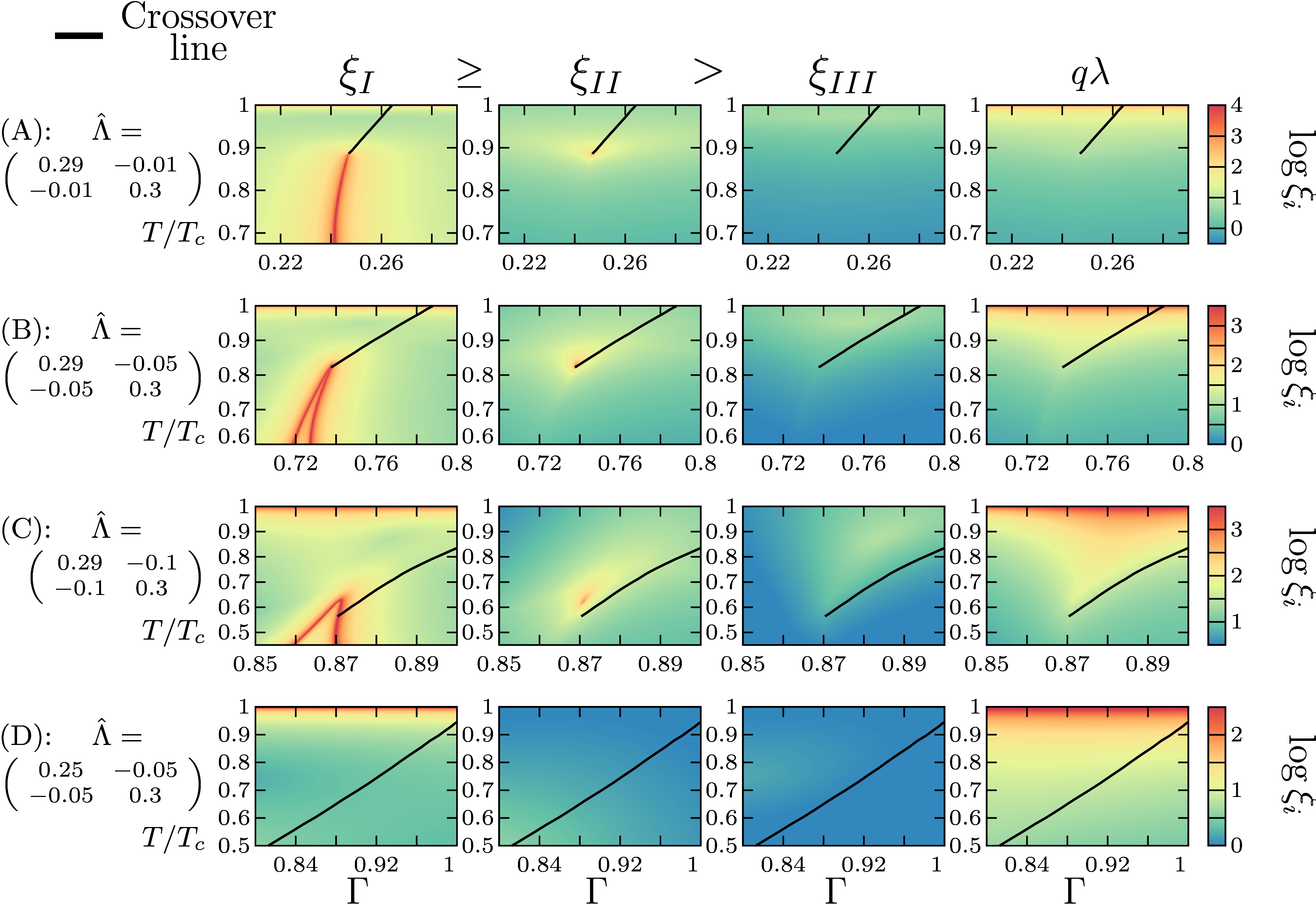
Figure 2: Physical length scales corresponding to various phase diagrams of the Ginzburg-Landau free energy (10). These are calculated from the eigenvalue problem (22). From left to right, the panels in the different columns show the three coherence lengths $\xi_{i}$ and the penetration depth $\lambda$, as functions of the temperature and interband scattering $\Gamma$. The lines correspond to different values of the coupling matrix $\hat{\lambda}$ that are displayed in Fig. 1. Namely lines (A), (B), and (C) correspond to nearly degenerate bands with weak, intermediate and strong repulsive interband pairing interaction respectively. Panel (D) describes the case of intermediate band disparity with intermediate repulsive interband pairing interaction. The ratio of diffusivities here is set to $r_{d}=1$ and the solid black line shows the crossover between $s_{\pm}$ and $s_{++}$ states. The largest coherence length ($\xi_{I}$) diverges both at $T_{c}$ and and the transition lines from $s_{++}/s_{\pm}$ to the time-reversal symmetry breaking $s+is$ state, indicating a second order phase transition. Interestingly, the second largest length scale $\xi_{II}$ also diverges in a single point of the phase diagram corresponding to the summit of the $s+is$ dome. Note the absence of any strong features of coherence lengths at the crossover line between $s_{\pm}$ and $s_{++}$ states. Note also that since the minority component vanishes at the crossover line, this illustrates that coherence length estimates $\xi\propto 1/\Delta$ cannot be used in multiband systems.

Figure 2 shows such length scales in the case of ratio of diffusivities $r_{d}=1$, as functions of the temperature and interband scattering $\Gamma$. First of all, as can be seen in the first and last column of Fig. 2, both the largest coherence length ($\xi_{I}$) and the penetration depth $\lambda$ naturally diverge at $T_{c}$, thus signaling the restoration of the $\mathrm{U}(1)$ symmetry via a second order phase transition. The model features additional phase transition associated with the time-reversal symmetry breaking: from $s_{++}/s_{\pm}$ (that breaks $\mathrm{U}(1)$) to the $s+is$ state (that breaks $\mathrm{U}(1)\times\mathbb{Z}_{2}$). If this phase transition is second order then the largest coherence length ($\xi_{I}$) should be divergent at that line as well. Figure 2 shows that this is indeed the case. Similar conclusion on the order of the phase transitions was reached in Ref. Silaev et al., 2017 through analysis of the effective potential of the model. Note, however, that from the quantities reported in Ref. Silaev et al. (2017), one cannot deduce the coherence lengths because they depend on the gradient terms.

Interestingly, the second largest coherence length $\xi_{II}$ is always finite except at a single point of the phase diagram that corresponds to the summit of the $s+is$ dome, where $\xi_{II}$ also diverges. The shortest length scale ($\xi_{III}$) is always finite. As can be seen from the various panels in Fig. 2, all length scales are finite at the crossover lines (denoted by the solid black line), where one of the gap vanishes.

Physical interpretations of the different coherence lengths can be deduced from the analysis of eigenvectors that correspond to the normal modes. First of all, one should emphasize that the eigenvectors of (22) are expressed in the rotated basis, and thus do not have a direct physical interpretation in terms of the original pairing gaps fields. Thus the eigenvectors of perturbation operator (22) should be expressed in the original basis. In analogy with the perturbative expansion (21) in the rotated basis, the fields in the original basis are expanded in small perturbations around the ground state, as

$$|\Delta_{i}|=U_{i}+\epsilon\delta|\Delta_{i}|\,,\leavevmode\nobreak\ \leavevmode\nobreak\ \theta_{12}={\bar{\theta}}+\epsilon\delta\theta_{12}\,.$$ (25)

There $U_{i}$ and ${\bar{\theta}}$ denote the ground state while $\delta|\Delta_{i}|$ and $\delta\theta_{12}$, stand for the perturbations in the original basis, and $\epsilon$ is the small parameter of the series expansion. The detailed expressions of the perturbations in the original basis can be found in the Appendix C. It is also convenient to introduce the perturbations associated to the total ($\delta|\Delta_{+}|$) and relative ($\delta|\Delta_{-}|$) density variations, defined as $\delta|\Delta_{\pm}|=\delta|\Delta_{1}|\pm\delta|\Delta_{2}|$.

Now, given the infinitesimal perturbations (25), in terms of the perturbations $f_{i}$ and $\phi$ of the rotated basis, we can investigate the behavior of the length scales and their corresponding physical modes. Fig. 3 shows the length scales and the corresponding modes as functions of the temperature for a given interband scattering $\Gamma=0.7275$. This corresponds to a vertical scan in the panel (B) of diagram Fig. 1, going across $s_{\pm}$, $s+is$ and $s_{++}$ phase. That vertical scan, covers four qualitatively different regimes. At low temperature, the system is in the $s_{++}$ state. The eigenmode associated with the largest length scale actually changes its nature during that scan. Indeed, the mode associated with with the divergent length scale at $T_{c}$ is a total amplitude mode, while the one that diverges at the $s+is$ transition is related to the relative phases. It is thus convenient to label the modes by their “critical” behavior. For example $\Upsilon_{T_{c}}^{\text{crit.}}$ is the mode that is associated with the length scale that diverges at $T_{c}$. The choice, Fig. 3, of two different background colors for the $s_{\pm}$ phase is to emphasize this fact that the mode $\Upsilon_{T_{c}}^{\text{crit.}}$ that dominates in the vicinity of $T_{c}$ has a completely different nature than $\Upsilon_{s+is}^{\text{crit.}}$ that is critical at the $s+is$ transition.

Interestingly, in the $s_{++}/s\pm$ phases, the mode $\Upsilon_{s+is}^{\text{crit.}}$ contributes both to relative phase and relative densities, and is decoupled from the total density variations. This picture produced by impurity-scattering is in contrast to clean two-band case Leggett (1966) where phase difference is fully decoupled from densities at linear level. Thus starting from low temperature, state in the $s_{++}$ phase, $\Upsilon_{s+is}^{\text{crit.}}$ does not contribute to the total density, but couples relative phase and relative density. At a higher temperature a second order phase transition to the time-reversal symmetry breaking $s+is$ state occurs, signaled by the divergence of the largest coherence length. In the $s+is$ state, all the modes contribute to the density modes (total and relative) and to the relative phase excitations as well. Further increasing the temperature drives the system through another second order phase transition to the $s_{\pm}$ state. Importantly, when approaching $T_{c}$, the critical mode at $s+is$ transition $\Upsilon_{s+is}^{\text{crit.}}$ that was dominating becomes subdominant in favor of $\Upsilon_{T_{c}}^{\text{crit.}}$, a pure density (amplitude) mode that is relevant for the restoration of the normal state.

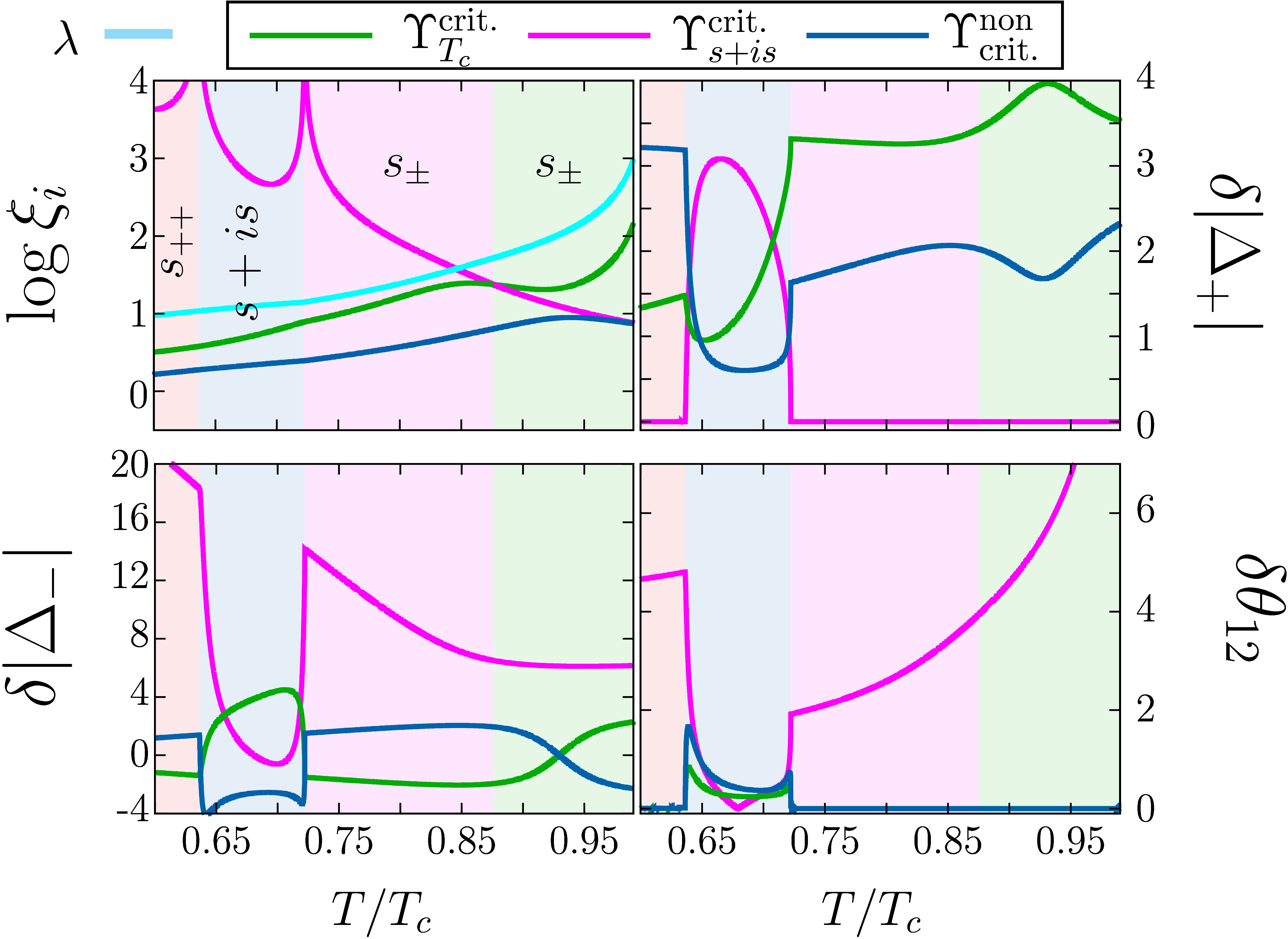
Figure 3: Behavior of the magnetic field penetration length, the coherence lengths and their associated normal modes, in a dirty two-band superconductor with nearly degenerate bands and intermediate repulsive interband pairing interaction (corresponding to panel (B) of diagram Fig. 1). The first panel shows the penetration depth and the three coherence lengths, as functions of the temperature, and for a fixed interband impurity scattering $\Gamma=0.7275$. It thus corresponds to a vertical scan in Fig. 1(B). There are different normal modes that are associated with the different coherence lengths. The green curve refers to the mode $\Upsilon_{T_{c}}^{\text{crit.}}$, whose coherence length diverges at $T_{c}$, that is critical at the superconducting phase transition. The pink curve is associated with $\Upsilon_{s+is}^{\text{crit.}}$, the mode whose coherence length diverges at the breakdown of time-reversal symmetry. The blue curve correspond to the mode that is not critical. The last three panels thus display the contributions of the different normal modes $\Upsilon$ to the infinitesimal perturbations $\delta|\Delta_{+}|$, $\delta|\Delta_{-}|$ and $\delta\theta_{12}$. Note that as $\Upsilon$ are eigenvectors or a linear operator, they are defined up to a normalization factor and only their relative contributions are meaningful. The different background colors denote different physical regimes. The $s_{++}$ state is realized at lowest temperatures, then the time-reversal symmetry breaking $s+is$ state occurs for an intermediate temperature range and is delimited by two second order phase transitions with a diverging coherence length. Finally, the $s_{\pm}$ is realized until $T_{c}$ where another second order phase transition occurs. Note that within the $s\pm$ phase, there are two different background colors. This stresses that the mode which is critical at $T_{c}$, $\Upsilon_{T_{c}}^{\text{crit.}}$, is essentially different from $\Upsilon_{s+is}^{\text{crit.}}$, the critical mode at the $s+is$ transition. Thus the green (resp. pink) background denotes the regions where $\Upsilon_{T_{c}}^{\text{crit.}}$ (resp. $\Upsilon_{s+is}^{\text{crit.}}$) dominates.

The results of the length scale analysis reported in Figs. 2 and 3 are performed for equal electron diffusivities in the different bands ($r_{d}=1$). Varying the relative diffusion constant alter the results only quantitatively, while the overall picture described above remains qualitatively the same. Quantitative detail on the influence of the relative diffusion constant $r_{d}$ on the length scales and on the upper critical field are reported in Appendix E. The analysis above shows that, at the linear level, the normal modes of a dirty two-band superconductor always couple the density and the relative phase excitations. Therefore such system does not feature a phase-only Leggett’s mode. This has to be contrasted with the case of similar but clean two-band system Silaev and Babaev (2011, 2012), where the Leggett’s modes and density modes always decouple.

Complicated variations of the coherence lengths in the dirty case, as well as the existence of diverging coherence lengths, are consequences of competing $s_{\pm}$ and $s_{++}$ and the $s+is$ states. They should have physical manifestations through the various responses that involve spatial or dynamical variations of the fields. Although their detailed analysis is beyond the scope of the current paper, we mention a few phenomena that can arise as a consequence of the rich interplay of the normal modes and their corresponding length scales. The above calculations do not consider dynamics but it demonstrates the existence of massless and soft dynamical modes that can be directly probed in experiment Blumberg et al. (2007).The mixed modes also dictate nontrivial thermoelectric properties Garaud et al. (2016a); Silaev et al. (2015) and their softening manifests itself in anomalies of flux flow viscosity Silaev and Babaev (2013). Likewise by the same mechanism the mode mixing produces nontrivial magnetic signatures of impurities Lin et al. (2016); Maiti et al. (2015), we discuss this in more detail below. Another interesting feature, that follows from the fact that one length scale diverges near the transition to the $s+is$ state, is that it can result in a particular length scale hierarchy where the magnetic field penetration length becomes an intermediate length scale. In the next section we consider implications of such a length scale hierarchy on vortex matter, and in particular illustrate that some behavior that can be deduced from the length scale analysis, actually survive beyond the linear regime.

IV Vortices in the vicinity of the $s+is$ region, physics beyond the linear regime

Here we discuss the physical properties associated with the topological excitations of dirty two-band superconductors, especially focusing on the possible consequences of the presence of the $s+is$ critical line on the phase diagram. We thus construct vortex solution by numerically minimizing the free energy (10). The physical degrees of freedom $\Delta_{1}$, $\Delta_{2}$ and ${\bm{A}}$ are discretized using finite-element formulation Hecht (2012), and the free energy is minimized using a non-linear conjugate gradient algorithm. To construct vortex solutions the minimization procedure is started with an initial configuration, in which both components $\Delta_{1}$ and $\Delta_{2}$ have the same vorticity. This initial vorticity specify the number of vortices that originally seeded in the numerical grid. The minimization procedure leads, after convergence of the algorithm, to a vortex configuration that carries the number of flux quanta that was specified by the initial phase winding. Note that the numerical grid has to be chosen much larger than the vortex configurations that are constructed. This is important to ensure that vortex matter do not interact with the domain boundaries and thus that the obtained configurations are not artifacts of boundary interactions. In particular, in the results that are displayed below, the numerical grid is larger than the displayed region which are close up views of the regions carrying vortices [Forfurtherdetailsonthenumericalmethodsemployedheresee; forexample; relateddiscussionin:][]Garaud.Babaev.ea:16. Note also that here we are interested in the physical properties of the vortex matter, such as intervortex forces, rather than magnetization process. This is why vortices are constructed here in zero external field, and seeded by the initial guess. By contrast in an external field, the vortex matter is not only subjected to its own intervortex interactions, but also to the interaction with Meissner currents, surface barriers, etc.

The determination of the length scales of the theory described in the previous section, relies on the linearization of the theory around the ground state. This analysis is thus relevant in the asymptotic regions that are far away from the vortex cores. As a result, the long-range intervortex interactions (that is, the interactions in the asymptotic region where the linear theory holds), are described in terms of the coherence lengths associated with the normal modes of the system [the solutions of the eigenproblem (22)]. Their nontrivial evolution and mixing across the phase diagram indicates the possible realization of nontrivial intervortex physics beyond the linear regime and thus a likely unusual magnetic magnetic response of the system. Because the dirty two-band superconductors described here feature a critical line that segregates the $s+is$ state from the other $s$-wave states, one coherence should diverge in the vicinity of that transition. Thus varying the temperature can drive the system from an $s$-wave state through the second order phase transition to the time-reversal symmetry-breaking $s+is$ state. Interestingly, as stressed in Fig. 3, for some fixed values of the impurity scattering rates, there can be two successive second order phase transitions: one from the $s_{\pm}\to s+is$ followed by a second $s+is\to s_{++}$ transition at lower temperature. As illustrated in Fig. 3, it immediately follows that a temperature-driven phase transition to the $s+is$ state goes along with the divergence of the largest coherence length at the transition line, while all other length scales, including the magnetic field’s penetration depth, remain finite.

Since the other length scales, including the magnetic field’s penetration length are finite at this transition, there are only two possible hierarchies of the length scales near that transition: (i) all coherence lengths are larger than $\lambda$ (which is a type-1 behavior), (ii) $\xi_{I}>\lambda$ but $\lambda$ is larger than some of the other coherence lengths. Since intervortex interactions are related to the long-range asymptotics, such a hierarchy of the length scales suggests long-range attractive, short-range repulsive intervortex forces. This regime was earlier termed “type-1.5” Moshchalkov et al. (2009) while associated phase separation was termed “semi-Meissner” state Babaev and Speight (2005)). As emphasized above, in dirty two-band superconductor, the normal mode with the largest coherence length typically mixes density modes and phase-difference mode. This implies that, in the vicinity of the $s+is$ transition, vortices feature a long-range tail of density suppression. This results in long-range attractive intervortex forces (dominated by the core-core interactions). On the other hand, at intermediate scales specified by the magnetic field’s penetration depth, the interactions are dominated by current-current interactions which are repulsive. The long-range intervortex interacting potential predicted by the linear theory can be expressed as a combination of modified Bessel functions of the second kind $K_{0}$, as:

$$U(r)=-C_{\lambda}^{2}K_{0}\left(\frac{r}{\lambda}\right)+\sum_{i=I,II,III}\left[C_{i}^{2}K_{0}\left(\frac{r}{\xi_{i}}\right)\right]\,.$$ (26)

The coefficients $C_{\lambda}$ and $C_{i}$ depend on the eigenstates of the perturbation operator (the normal modes) and on nonlinearities.

     

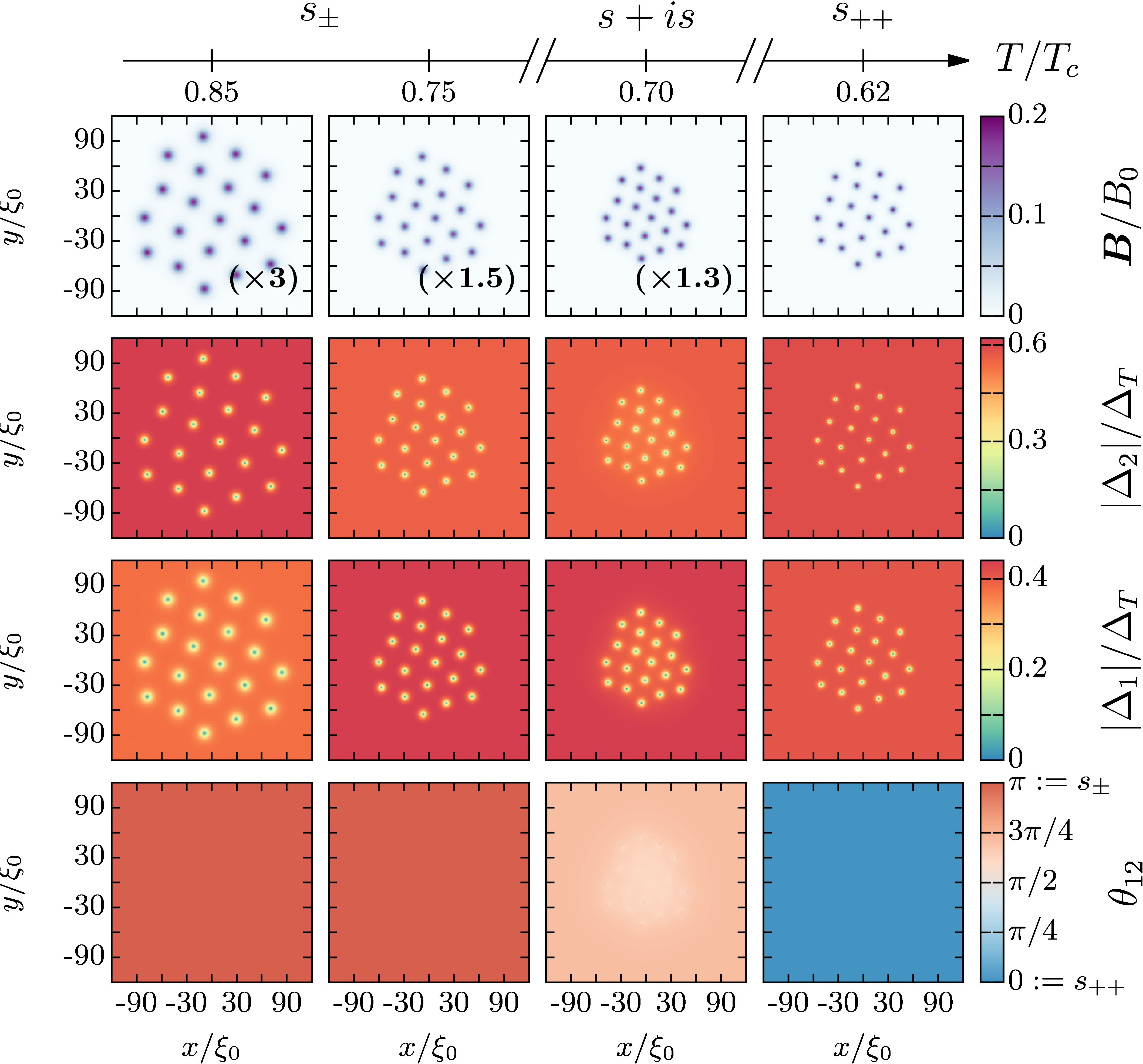
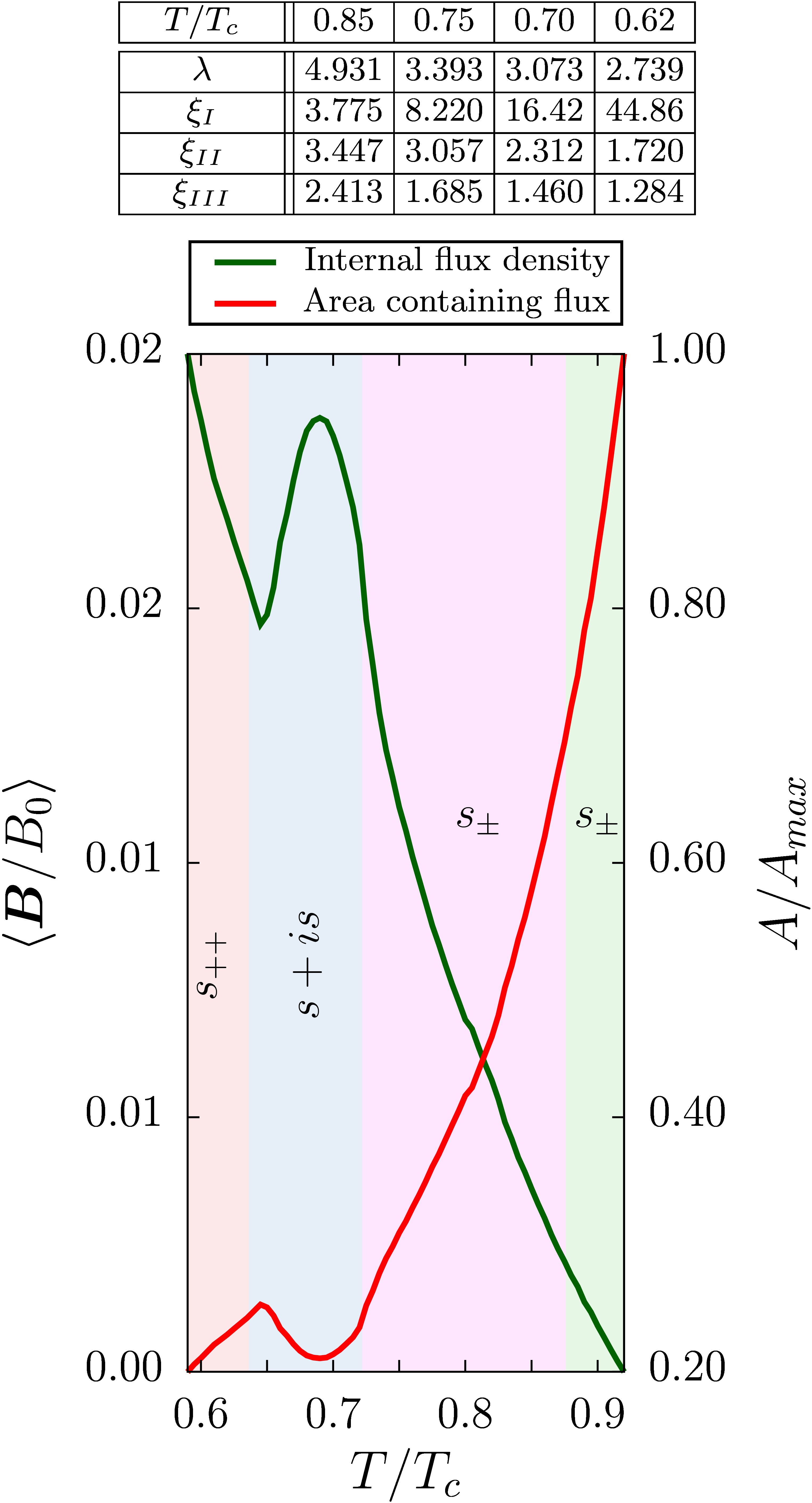
Figure 4: Evolution of bound state of 20 vortices during a cooling procedure like that displayed in Fig. 3. Apart from the temperature, all other paramaters are fixed: the interband scattering rate is $\Gamma=0.7275$, the gauge coupling constant is $q=0.5$, and electronic diffusivities are equal ($r_{d}=1$). On the left panel, the displayed quantities on the different lines are respectively the magnetic field ${\bm{B}}$, the amplitudes of the gap in majority ($|\Delta_{2}|$) and minority ($|\Delta_{1}|$) components. The last line shows the relative phase $\theta_{12}$ from which the ground state phase can be directly read. Different vortex configurations, at different temperatures, can be read from the various columns displayed on the left panel. The first column shows a type-2 regime where the largest length scale is the penetration depth and thus the repulsion forces dominate. The other columns, on the other hand, show the typical realization of a type-1.5 regime. There, due to the proximity with the $s_{++}/s_{\pm}\to s+is$ transition, the largest coherence length increases and this triggers the long-range attractive forces resulting in the formation of a compact cluster of vortices. The right panel shows the flux-carrying area (defined as the area of the region where the magnetic fields is above some threshold $\delta=0.005B_{max}$), and the internal mean magnetic flux density in the flux-carrying region. The internal flux density shows a strong peak where the attractive intervortex forces are strongest and thus the clusters are the most compact. Here this peak is near the $s+is$ transition. The numerical values of the various length scales corresponding to the different regimes displayed on the left panel are shown in the top right table.

Thus, in the vicinity of the second order phase transition to the time-reversal symmetry breaking $s+is$ state, the interplay between the long-range attraction driven by the core-core interactions, and the short-range repulsion due to the current-current repulsion, yields non-monotonic intervortex forces (cf. with calculations in different two-band models Babaev and Speight (2005); Babaev et al. (2010); Carlström et al. (2011b); Silaev and Babaev (2011).)

Such forces can promote the formation of a bound-state of vortices. In such a bound-state, the distance separating the vortices does not directly follow from linearized theory, but is determined by full nonlinear theory. As a result, since all the parameters of the Ginzburg-Landau model (10) are temperature dependent (see the exact formulas of the coefficients in Appendix A), it is quite expectable that if vortex bound-state are formed in the full nonlinear model, their typical size should also be temperature dependent.

Below, we present the results of such an analysis of the full nonlinear response in the Ginzburg-Landau model. Using the numerical procedure described earlier in this section, we systematically construct sets of several vortices for fixed impurity scattering rates and decreasing temperatures similar to the parameter set investigated in Fig. 3 (thus corresponding to a vertical scan in the phase diagrams Fig. 1). The situation that is considered now mimics a dilute groups of vortices that form in a field-cooled sample in fields far from upper critical magnetic field. Figure 4 displays the behavior of a set of $20$ vortices at different temperatures. The selected temperatures are representatives of the various phases shown in Fig. 3.

Depending on the regime, when starting from an initial set of $20$ vortices, the numerical procedure leads after convergence to a characteristic picture corresponding to either a type-2 regime or to vortex clusters that are typically realized in the type-1.5 regime. In the vicinity of the superconducting transition, as illustrated by the configuration in the first column of Fig. 4, which is close to $T_{c}$ and deep in the $s_{\pm}$ region, the vortex configuration is typical of a type-2 regime. Note that type-2 regime theoretically implies an infinite vortex separation, but the strength of the repulsion decays exponentially with the separation. So for all practical purposes, the repulsion between vortices ends when the strength becomes smaller than the numerical accuracy: that is similar to experimental situation of remnant vorticity where intervortex repulsion or vortex-boundary interaction is too small to reach truly lowest energy state.

Upon decreasing the temperature, the largest coherence length $\xi_{I}$ increases rapidly, as the system gets closer to the transition to the $s+is$ state. This triggers the expected long-range attractive mode which leads to the formation of a vortex cluster. The last three columns on the left panel of Fig. 4 correspond, at the linear level to type-1.5 regimes. In other words, as can be read from the values of the length scales on Fig. 2, the penetration depth there, is and intermediate length scale. The corresponding regimes in the last three columns of Fig. 4 show that, in the nonlinear regime, vortices aggregate in a cluster. As can be seen from the two central columns of Fig. 4, the vortex coalescence occurs near the phase transition to the $s+is$ state, and the most compact cluster forms in the $s+is$ phase (this can seen from the third column). Further decreasing of the temperature drives the system through another second-order phase transition to the $s_{++}$ state. While moving away from criticality, the largest coherence length shortens. Correspondingly, the range of attractive interaction also shortens, and the attractive forces weaken. Eventually, repulsive forces will become dominant again, and the set of vortices will fall back in a type-2 regime. Observe that Fig. 4 clearly shows that the scale of strong suppression of gaps in the vortex core is not directly related to coherence lengths.

For a system with non-monotonic interactions, standard kinetic mechanisms (see for example Sethna (2006)) leads to different patterns of phase coexistence. In the case studied here the vortex clusters coexist with domains of Meissner state. The temperature dependence of intervortex forces opens up a possibility to discriminate the effect described here from a phase separation originating in vortex pinning. The formation of vortex cluster can be probed by the direct vortex visualization techniques such as magnetooptics, scanning Hall, and scanning SQUID probes. This could also be experimentally probed for example in muon-spin rotation measurements ($\mu SR$) like the ones conducted in Ref. Ray et al. (2014). That is, when $\mu SR$ detects a phase separation into vortex clusters and Meissner domains, the above considered contraction of vortex cluster when the temperature is lowered, should result in a local increase of magnetic field: quantity that, again, can be extracted from $\mu SR$ data Ray et al. (2014). In order to connect the effect of vortex clusterization with this experimentally measurable quantity, we calculate the local mean magnetic flux density for vortex cluster as the system is cooled down. The evolution of the mean magnetic flux density of a cluster during the cool-down process is displayed on the right panel of Fig. 4. There is a strong peak in the magnetic flux density in correspondence to an increase of the vortex binding forces near the $s+is$ transition.

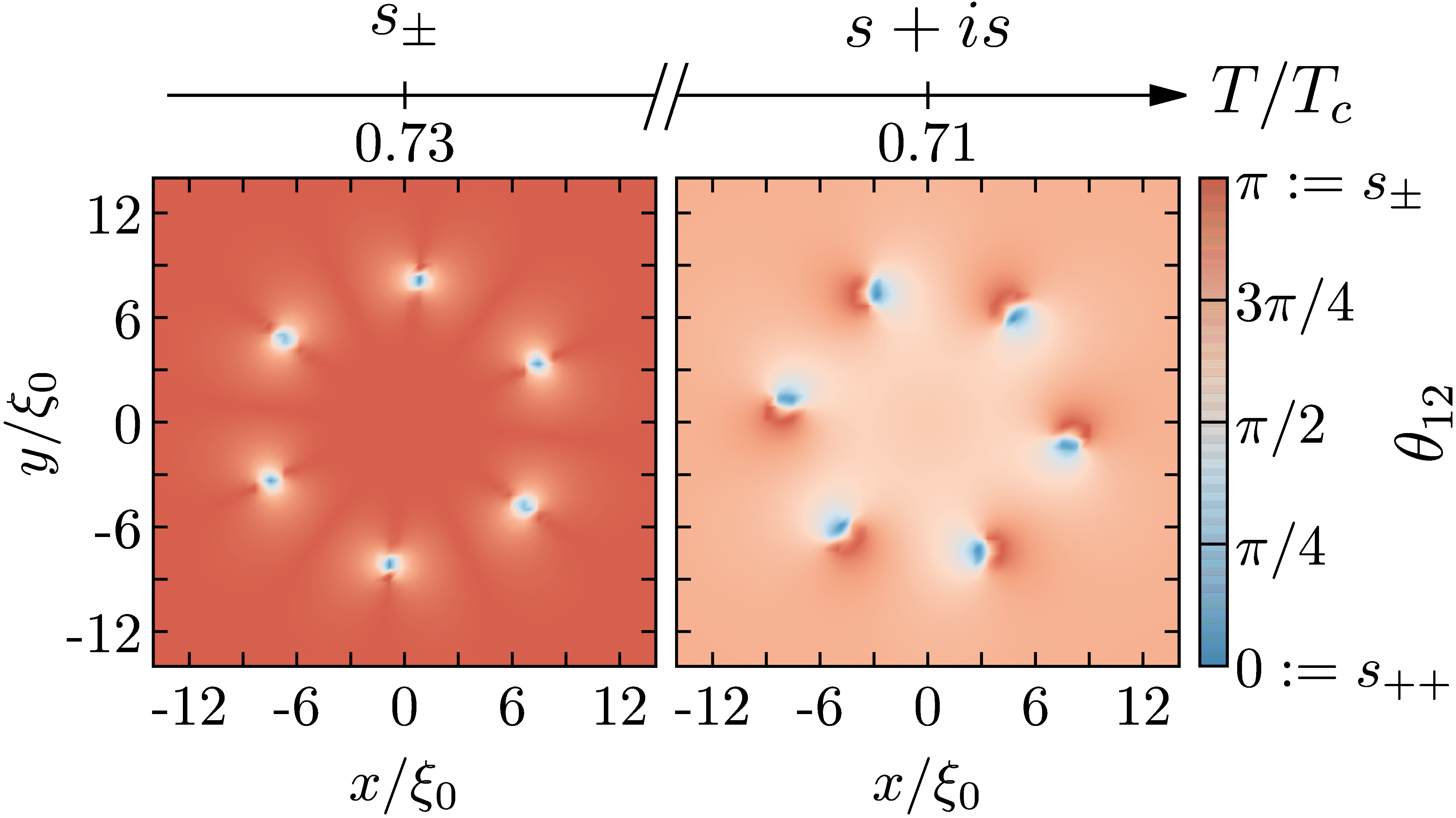
Figure 5: Splitting of composite integer flux quanta vortices into fractional vortices, at the boundary of clusters formed due to the long range attractive forces near the $s+is$ transition. Here a cluster of seven vortices for the same parameters as in Fig. 4 besides $q=0.8$, both in the $s_{\pm}$ state (first column) and $s+is$ (second column). The relative phase shows the splitting of vortices at the boundary of the cluster.

The appearance of this kind of signal assumes phase separation due to kinetic reasons. However similar signal should also be expected for dilute vortex lattices that can contract due to emerging attractive forces as well. The strength of the effect will also depend on the magnetic penetration lengths: the longer is $\lambda$, the weaker are the intervortex attractive forces. On the quantitative side: an interesting feature is the the vortex clusterization can start very far away from the $s+is$ phase transition. This is fully consistent with linear analysis where we find, in Fig. 3, a broad region of increased largest coherence length associated with the critical mode. Therefore even if the $s+is$ phase occupies an unobservably small domain on the phase diagram the soft modes implied by that criticality exist and modify magnetic response in a wide range of parameters.

Having established vortex clustering due to existence of a critical mode, we briefly discuss a few of structural features of vortex clusters. Detailed study of the vortex cluster structure is beyond the scope of this paper and is perhaps a fruitful direction of application of methods developed in research on filament bundles. Yet, it should be emphasized that indeed the vortex clusters are not a simple superposition of single vortex solutions. Correspondingly the equation (26), that is based on the linear theory with the assumption of axially symmetric composite vortices, can received nonlinear corrections. One of the possible nonlinear effect is that clusters can exhibit disintegration of the composite character of vortices: namely a small splitting of the vortex cores in the different components near clusters boundary. This behavior can clearly be seen in the numerical solutions shown in Fig. 5 for a cluster of seven vortices. As can be seen in Fig. 5, clearly the phenomena of vortex splitting occurs at the boundary, while the inner vortex sitting at the center of the cluster shows no splitting. Such a splitting of vortex cores at the boundary of clusters excites a mode that is not present in the interaction between single vortices, but that should contribute to the inter-cluster interactions.

It should finally be stressed the coherence lengths cannot be related in a simple way to overall vortex core sizes, because of the nonlinear nature of the coupled system. It can clearly be seen in Fig. 4 that although one of the length scales diverges in the vicinity of the $s+is$ transition, this has a relatively little influence on the size of substantial density suppression in vortex cores (but dramatically affects the long-range weak density suppression and thus the intervortex interactions).

V Effects of spatial gradients in impurity density

The previous sections describe the effect of impurities on the phase diagram of dirty two-band superconductors and, in particular, how it affects the different length scales. We further demonstrated that, in the vicinity of the impurity induced second order phase transition associated with the spontaneous breakdown of the time-reversal symmetry, it results in non-monotonic intervortex forces that can lead to the formation of vortex clusters whose typical signature can in principle be probed in $\mu$SR measurements.

Figure 6: Appearance of spontaneous magnetic fields and fragmentation of vortex cluster due to small periodic modulation of the impurity scattering rate $\Gamma$. All the microscopic parameters are the same as in Fig. 4. The temperature is $T/T_{c}=0.7$, while the impurity scattering strength is modulated sinusoidally with amplitudes $\Gamma=0.7275\pm 0.02$. The panels on the top row show the modulated impurity and the induced magnetic field, in the absence of vortices. The middle line displays the amplitudes of the gap in minority ($|\Delta_{1}|$) and majority components ($|\Delta_{2}|$) of the fragmented of vortex cluster. The bottom row shows the corresponding magnetic field ${\bm{B}}$ and the relative phase $\theta_{12}$. Modulation of impurity provides a pinning landscape that favors placing vortices where the impurity is increased, and this tends to break cluster into smaller clusters, as compared to Fig. 4. Nonetheless the clearly large areas of gap suppression indicates the presence of attractive intervortex forces. In addition the modulation of $\Gamma$ produces a small spontaneous magnetic field in the $s+is$ state as can be seen from the second top panel. Note however that the spontaneous field is several orders of magnitude smaller than that of vortices, and it is typically dominated by the vortex background.

The discussion so far focused on the case of a spatially uniform distribution of impurity density. It is instructive to consider one more example, where the impurity density is not uniformly distributed in space. Spatially varying impurity will result in an inhomogeneous superconducting state which will feature gradients both of densities and relative phases of the field components as a consequence of mode mixing. This in turn can produce spontaneous magnetic fields. Spontaneous magnetic fields were indeed shown to occur in various models of $s+is$ states for different kind of inhomogeneities such as impurities and domain walls and their combinations Garaud and Babaev (2014); Maiti et al. (2015); Lin et al. (2016); Vadimov and Silaev (2018), and impurity-like inhomogeneities produced by the local heating of a superconductor Silaev et al. (2015); Garaud et al. (2016a). In this section we report that spontaneous magnetic fields arise when there are gradients of impurity density. The magnetic field discussed in the previous section will be superimposed with the spontaneous magnetic field. This can have direct implications for the vortex states previously considered, since both the inhomogeneities and the spontaneous magnetic fields induced by them can provide a pinning landscape for vortices.

To illustrate that inhomogeneities can indeed yield spontaneous magnetic fields, we consider an idealized situation of a sinusoidal modulation of the impurity scattering rates $\Gamma=0.7275\pm 0.02$, where the period of the modulation is of the order of the size of a vortex. Figure 6 shows this situation, where spontaneous magnetic field appears due to the modulation of impurities. Moreover, it shows that it can also substantially affect vortex structures such as the clusters previously reported in Fig. 4. Indeed, in this example, inhomogeneities of the impurity scattering rates clearly result in the fragmentation of the vortex cluster into smaller clusters. In other words, inhomogeneities induce a pinning landscape due to gap modulations and due to appearance of spontaneous multipolar magnetic field, that affects the structure of vortex clusters.

The spontaneous magnetic field that arises exclusively due to inhomogeneities (i.e. without vortices) is displayed in the second panel of the first row of Fig. 6, and it is maximal where the modulation of $\Gamma$ has its larger gradients. The spontaneous magnetic field is spatially alternating and its total flux across the sample is zero in the absence of vortices. Note that there is an enhanced spontaneous field near the boundaries that is dipole-like, rather than quadrupole-like in the bulk. This is not a generic property, but rather a consequence of the particular choice of the modulation here that has stronger gradients whose contribution is less compensated at the boundary.

The presence of spatially inhomogeneous distribution of impurities can thus have experimental manifestations that can, for example, be detected in a zero field by $\mu SR$ and scanning SQUID experiments. Moreover, as can be seen from the other panels in Fig. 6, besides the spontaneous magnetic fields, the inhomogeneities can also act as a pinning landscape for vortices that will alter the structure of the clusters discussed in the previous section. Such a cluster fragmentation due to pinning should result in a reduction of the $\mu$SR signatures discussed in the previous section, in the case of homogeneous systems.

VI Conclusion

In conclusion, in this work we studied the properties of dirty two-band superconductors with repulsive interband interaction. We used the microscopically derived Ginzburg-Landau theory, to give qualitatively consistent solutions with Usadel model, not too far from superconducting $T_{c}$. We investigated the normal modes, and their corresponding coherence lengths. The normal modes of dirty systems are much more complex than those in clean two-band cases due to the frustration between various interband interaction terms. One of the new features is the mixing of the Leggett mode with the density modes that occurs even without time-reversal symmetry breaking. An important property of the dirty two-band superconductors is the presence of a region of $s+is$ state on the phase diagram. This $s+is$ domain is surrounded by a line of second order phase transition that dictates the existence of a soft mode and an infinite disparity of coherence lengths. A striking feature is that the disparity of the coherence lengths and relatively soft mode persists for a wide range of coupling constants and temperatures, even if the domain of the $s+is$ phase is too small to be directly resolvable in experiment. This, makes such systems very different from the clean two-band $s$-wave case Silaev and Babaev (2011). This should also have consequences for various properties associated with the static and dynamic fluctuations. We focused here on consequences to the vortex physics and demonstrated the existence of a region where the hierarchy of the length scales is such that the penetration depth becomes an intermediate length scale (the so-called type-1.5 regime). This leads to long-range attractive and short-range repulsive intervortex forces, leading to formation of vortex bound states or clusters. These clusters, due to the temperature dependence of the mean magnetic field’s density, have specific signatures that can be discriminated from other mechanisms also responsible of cluster formation. This should be experimentally measureable in muon-spin-rotation experiments. Note finally that qualitatively similar features should also be expected in other realizations of $s+is$ states Ng and Nagaosa (2009); Stanev and Tešanović (2010); Carlström et al. (2011a); Maiti and Chubukov (2013); Böker et al. (2017); Grinenko et al. (2017).

Appendix A Ginzburg-Landau coefficients

There, the coefficients of the Ginzburg-Landau functional $a_{ij}$, $b_{ij}$, $c_{ij}$ and $k_{ij}$ can be calculated from the inputs $\lambda_{ij}$, $T$ and $\Gamma$ of the microscopic self-consistency equation. $N_{i}$ are the densities of states and $D_{i}$ the electron diffusivities. First, the coefficients of gradient terms are given by Garaud et al. (2017)

$$k_{ii} =2\pi TN_{i}\sum_{n=0}^{N_{d}}\frac{D_{i}(\omega_{n}+\gamma_{ji})^{2}+\gamma_{ij}\gamma_{ji}D_{j}}{\omega^{2}_{n}(\omega_{n}+\gamma_{ij}+\gamma_{ji})^{2}}$$ (A27a)

$$k_{ij} =2\pi TN_{i}\gamma_{ij}\sum_{n=0}^{N_{d}}\frac{D_{i}(\omega_{n}+\gamma_{ji})+D_{j}(\omega_{n}+\gamma_{ij})}{\omega^{2}_{n}(\omega_{n}+\gamma_{ij}+\gamma_{ji})^{2}}\,,$$ (A27b)

with $j\neq i$. The coefficients of the potential terms can be found for example from Ref. Stanev and Koshelev, 2014 and they read as

$$a_{ii} =\frac{N_{i}\lambda_{jj}}{\mathrm{det}(\hat{\lambda})}-2\pi T\sum_{n=0}^{N_{d}}\frac{(\omega_{n}+\gamma_{ji})N_{i}}{\omega_{n}(\omega_{n}+\gamma_{ij}+\gamma_{ji})}\,,$$ (A28a)

$$a_{ij} =-\frac{N_{i}\lambda_{ij}}{\mathrm{det}(\hat{\lambda})}-2\pi T\sum_{n=0}^{N_{d}}\frac{\gamma_{ij}N_{i}}{\omega_{n}(\omega_{n}+\gamma_{ij}+\gamma_{ji})}\,.$$ (A28b)

The other parameters read as

$$b_{ii} =\pi TN_{i}\sum_{n=0}^{N_{d}}\frac{(\omega_{n}+\gamma_{ji})^{4}}{\omega_{n}^{3}(\omega_{n}+\gamma_{ij}+\gamma_{ji})^{4}}$$ (A29a)

$$\leavevmode\nobreak\ +\pi TN_{i}\sum_{n=0}^{N_{d}}\frac{\gamma_{ij}(\omega_{n}+\gamma_{ji})(\omega_{n}^{2}+3\omega_{n}\gamma_{ji}+\gamma_{ji}^{2})}{\omega_{n}^{3}(\omega_{n}+\gamma_{ij}+\gamma_{ji})^{4}}\,,$$

$$b_{ij} =-\pi TN_{i}\sum_{n=0}^{N_{d}}\frac{\gamma_{ij}}{(\omega_{n}+\gamma_{ij}+\gamma_{ji})^{4}}$$ (A29b)

$$+\pi TN_{i}\sum_{n=0}^{N_{d}}\frac{\gamma_{ij}(\gamma_{ij}+\gamma_{ji})(\omega_{n}(\gamma_{ij}+\gamma_{ji})+2\gamma_{ij}\gamma_{ji})}{\omega_{n}^{3}(\omega_{n}+\gamma_{ij}+\gamma_{ji})^{4}}\,,$$

and

$$c_{ii} =\pi TN_{i}$$ (A30a)

$$\sum_{n=0}^{N_{d}}\frac{\gamma_{ij}(\omega_{n}+\gamma_{ji})(\omega_{n}^{2}+(\omega_{n}+\gamma_{ji})(\gamma_{ij}+\gamma_{ji}))}{\omega_{n}^{3}(\omega_{n}+\gamma_{ij}+\gamma_{ji})^{4}}\,,$$

$$c_{ij} =\pi TN_{i}\sum_{n=0}^{N_{d}}\frac{\gamma_{ij}(\omega_{n}+\gamma_{ji})(\omega_{n}+\gamma_{ij})(\gamma_{ij}+\gamma_{ji})}{\omega_{n}^{3}(\omega_{n}+\gamma_{ij}+\gamma_{ji})^{4}}\,.$$ (A30b)

Thus for a given set of input microscopic parameters, $\lambda_{ij}$, $\Gamma$ and $T$ close to $T_{c}$, we can reconstruct the coefficients (A27)–(A30) and investigate the ground-state properties of the GL theory by minimizing the free energy (10) with respect to $|\Delta_{j}|$ and $\theta_{12}$.

Appendix B Ginzburg-Landau coefficients of the mixed-gradients-free basis

Rewriting the original Ginzburg-Landau model (10), using a linear combination of the components of the order parameter:

$$\psi_{1} =\sqrt{k_{11}}\Delta_{1}+\sqrt{k_{22}}\Delta_{2}\,,$$ (B31a)

$$\psi_{2} =\sqrt{k_{11}}\Delta_{1}-\sqrt{k_{22}}\Delta_{2}\,,$$ (B31b)

allows a much simpler form of the kinetic terms which is convenient to investigate physical length scales. Within the new basis, the coefficients for the kinetic term of the rewritten Ginzburg-Landau functional (13) read as:

$$\kappa_{1}=\frac{\sqrt{k_{11}k_{22}}+k_{12}}{2\sqrt{k_{11}k_{22}}}\leavevmode\nobreak\ \leavevmode\nobreak\ \leavevmode\nobreak\ \leavevmode\nobreak\ \text{and}\leavevmode\nobreak\ \leavevmode\nobreak\ \leavevmode\nobreak\ \leavevmode\nobreak\ \kappa_{2}=\frac{\sqrt{k_{11}k_{22}}-k_{12}}{2\sqrt{k_{11}k_{22}}}\,.$$ (B32)

The coefficients of the potential read as

$$\alpha_{11} =\frac{a_{11}k_{22}+a_{22}k_{11}+2a_{12}\sqrt{k_{11}k_{22}}}{4k_{11}k_{22}}\,,$$ (B33a)

$$\alpha_{22} =\frac{a_{11}k_{22}+a_{22}k_{11}-2a_{12}\sqrt{k_{11}k_{22}}}{4k_{11}k_{22}}\,,$$ (B33b)

$$\alpha_{12} =\frac{a_{11}k_{22}-a_{22}k_{11}}{4k_{11}k_{22}}\,,$$ (B33c)

and

$$\beta_{11} =\frac{b_{11}k_{22}^{2}+b_{22}k_{11}^{2}}{16k_{11}^{2}k_{22}^{2}}+\frac{b_{12}+c_{12}}{8k_{11}k_{22}}+\frac{c_{11}k_{22}+c_{22}k_{11}}{4(k_{11}k_{22})^{3/2}}\,,$$ (B34a)

$$\beta_{22} =\frac{b_{11}k_{22}^{2}+b_{22}k_{11}^{2}}{16k_{11}^{2}k_{22}^{2}}+\frac{b_{12}+c_{12}}{8k_{11}k_{22}}-\frac{c_{11}k_{22}+c_{22}k_{11}}{4(k_{11}k_{22})^{3/2}}\,,$$ (B34b)

$$\beta_{12} =\frac{b_{11}k_{22}^{2}+b_{22}k_{11}^{2}}{8k_{11}^{2}k_{22}^{2}}-\frac{c_{12}}{4k_{11}k_{22}}\,.\leavevmode\nobreak\$$ (B34c)

Finally

$$\gamma_{11} =\frac{b_{11}k_{22}^{2}-b_{22}k_{11}^{2}}{16k_{11}^{2}k_{22}^{2}}+\frac{c_{11}k_{22}-c_{22}k_{11}}{8(k_{11}k_{22})^{3/2}}\,,$$ (B35a)

$$\gamma_{22} =\frac{b_{11}k_{22}^{2}-b_{22}k_{11}^{2}}{16k_{11}^{2}k_{22}^{2}}-\frac{c_{11}k_{22}-c_{22}k_{11}}{8(k_{11}k_{22})^{3/2}}\,,$$ (B35b)

$$\gamma_{12} =\frac{b_{11}k_{22}^{2}+b_{22}k_{11}^{2}}{16k_{11}^{2}k_{22}^{2}}+\frac{c_{12}-b_{12}}{8k_{11}k_{22}}\,.$$ (B35c)

Appendix C Perturbations in the original basis

Using the equations (21) and (25), the perturbations are reconstructed, and they are expressed in terms of the perturbations in the rotated basis, as

$$\delta|\Delta_{1}|^{2} =\frac{1}{2k_{11}}\left(\frac{f_{1}^{2}}{\kappa_{1}^{2}}+\frac{f_{2}^{2}}{\kappa_{2}^{2}}\right)$$ (C36a)

$$-\left(\frac{u_{1}f_{2}}{\kappa_{2}}+\frac{u_{2}f_{1}}{\kappa_{1}}\right)\sqrt{\frac{\kappa_{1}u_{1}^{2}+\kappa_{2}u_{2}^{2}}{k_{11}^{2}\kappa_{1}^{3}\kappa_{2}^{3}u_{1}^{2}u_{2}^{2}}}\sin{\bar{\varphi}}\phi$$

$$-\frac{1}{k_{11}\kappa_{1}\kappa_{2}}\left(\left(f_{1}f_{2}+\frac{\kappa_{1}u_{1}^{2}+\kappa_{2}u_{2}^{2}}{2u_{1}u_{2}}\right)\cos{\bar{\varphi}}\right)\,,$$

$$\delta|\Delta_{2}|^{2} =\frac{1}{2k_{22}}\left(\frac{f_{1}^{2}}{\kappa_{1}^{2}}+\frac{f_{2}^{2}}{\kappa_{2}^{2}}\right)$$ (C36b)

$$+\left(\frac{u_{1}f_{2}}{\kappa_{2}}+\frac{u_{2}f_{1}}{\kappa_{1}}\right)\sqrt{\frac{\kappa_{1}u_{1}^{2}+\kappa_{2}u_{2}^{2}}{k_{22}^{2}\kappa_{1}^{3}\kappa_{2}^{3}u_{1}^{2}u_{2}^{2}}}\sin{\bar{\varphi}}\phi$$

$$+\frac{1}{k_{22}\kappa_{1}\kappa_{2}}\left(\left(f_{1}f_{2}+\frac{\kappa_{1}u_{1}^{2}+\kappa_{2}u_{2}^{2}}{2u_{1}u_{2}}\right)\cos{\bar{\varphi}}\right)\,,$$

$$\delta\theta_{12} =\frac{-2u_{1}u_{2}(u_{1}^{2}+u_{2}^{2})\cos{\bar{\varphi}}\sqrt{\frac{\kappa_{1}u_{1}^{2}+\kappa_{2}u_{2}^{2}}{\kappa_{1}\kappa_{2}u_{1}^{2}u_{2}^{2}}}\phi}{(u_{1}^{2}+u_{2}^{2})^{2}+4u_{1}^{2}u_{2}^{2}\sin^{2}{\bar{\varphi}}}$$

$$\leavevmode\nobreak\ -\frac{2u_{1}u_{2}(u_{1}-u_{2})\left(\frac{u_{1}f_{2}}{\kappa_{2}}-\frac{u_{2}f_{1}}{\kappa_{1}}\right)}{(u_{1}^{2}+u_{2}^{2})^{2}+4u_{1}^{2}u_{2}^{2}\sin^{2}{\bar{\varphi}}}\,.$$ (C36c)

Appendix D Second critical field

$\mathrm{H}_{c2}$ can be obtained by considering the perturbation operator around the normal state. More precisely, in the original parametrization the normal state is $|\Delta_{1}|=|\Delta_{2}|=0$. Using (III.1), this implies that the normal state in the new variables is $|\psi_{1}|=|\psi_{2}|=0$ and thus $u_{1}=u_{2}=0$ and ${\bar{\varphi}}=0$.

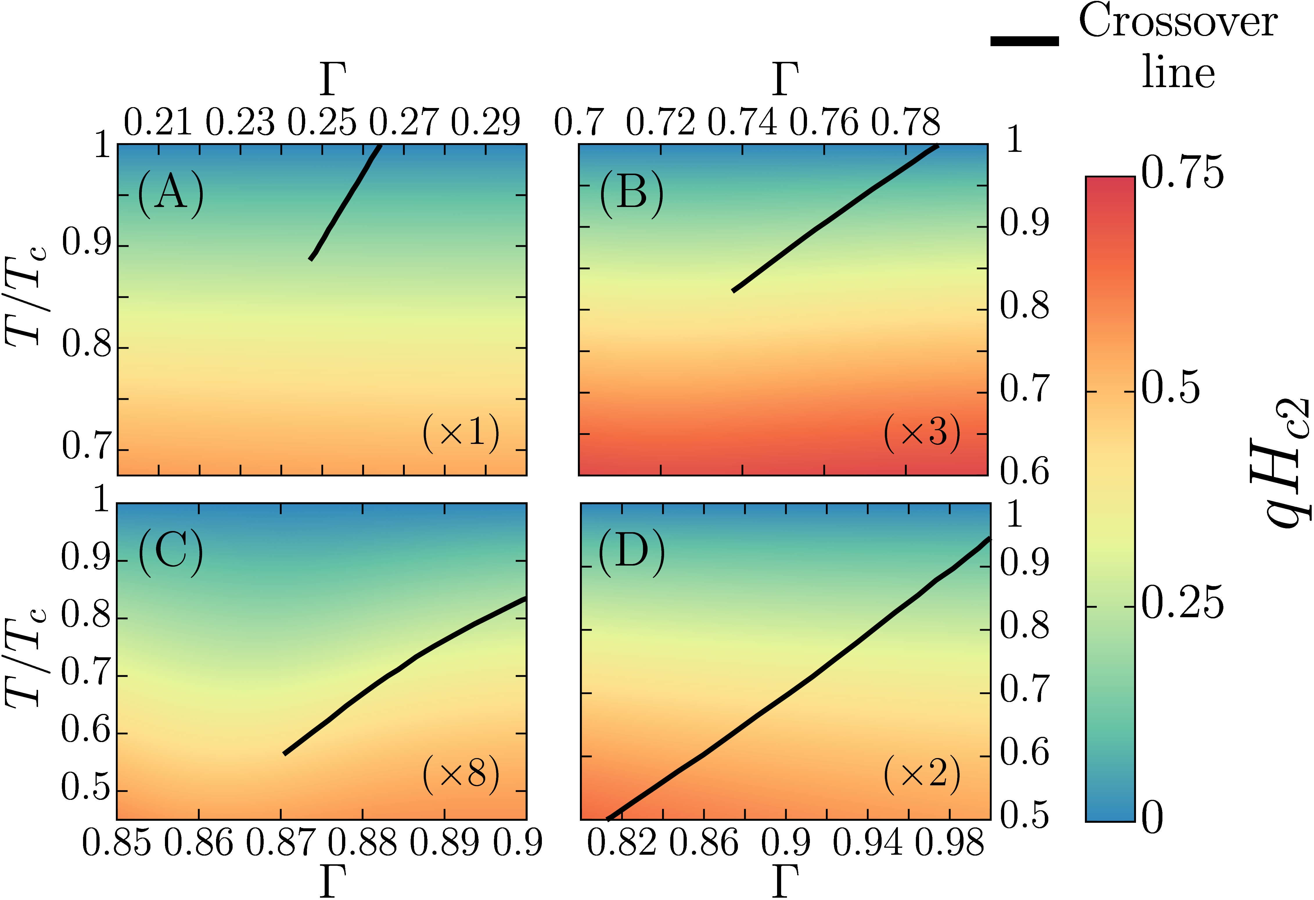
Figure 7: Upper critical field $\mathrm{H}_{c2}$, as defined in (D43), as a function of temperature and interband scattering $\Gamma$, for equal diffusivities in both bands ($r_{d}=1$). The different panels correspond to different values of the coupling matrix $\hat{\lambda}$ that are displayed in Fig. 1. Clearly, the complexity of the phase diagram of the model has little effect on the behavior of $\mathrm{H}_{c2}$.

Close to the second critical field $\mathrm{H}_{c2}$ the magnetic field is approximately constant: ${\bm{B}}=B_{0}{\bm{e}}_{z}$ and the densities are small. Thus the Ginzburg-Landau equations (15) can be linearized around the normal state as

$$\Pi^{2}\Upsilon={\cal M}^{2}\big{\rvert}_{u_{1}=u_{2}={\bar{\varphi}}=0}\Upsilon\equiv{\cal M}_{0}^{2}\Upsilon\,.$$ (D37)

Because of the gauge invariance, the vector potential can be parametrized in the Landau Gauge as ${\bm{A}}=(0,B_{0}x,0)^{-1}$. As a result, the linearized Ginzburg-Landau equations read as

$$\left({\bm{\nabla}}^{2}-\left(qB_{0}x\right)^{2}\right)\Upsilon={\cal M}_{0}^{2}\Upsilon\,.$$ (D38)

For the simple Gaussian ansatz $\Upsilon=C\exp\left(-\frac{x^{2}}{2\xi^{2}}\right)$ with the vector $C=(C_{1},C_{2})^{T}$ and $qB_{0}=1/\xi^{2}$. The equation (D38) further simplifies:

$${\cal M}_{0}^{2}\Upsilon=\frac{-1}{\xi^{2}}\Upsilon\,.$$ (D39)

Thus $1/\xi^{2}$ is an eigenvalue of $-{\cal M}_{0}^{2}$. More precisely, its largest:

$$q\mathrm{H}_{c2}=\frac{1}{\xi^{2}}:=\mathrm{max}\Big{(}\mathrm{Eigenvalue}\big{[}-{\cal M}_{0}^{2}\big{]}\Big{)}\,.$$ (D40)

It is easy to realize that the perturbations of the relative phase $\Upsilon$ decouple from density perturbations. The mass matrix thus becomes:

$${\cal M}_{0}^{2}=2\left(\begin{array}[]{cc}\alpha_{11}/\kappa_{1}&\alpha_{12}/\sqrt{\kappa_{1}\kappa_{2}}\\ \alpha_{12}/\sqrt{\kappa_{1}\kappa_{2}}&\alpha_{22}/\kappa_{2}\end{array}\right)\,,$$ (D41)

and its eigenvalues are

$$\frac{\kappa_{2}\alpha_{11}+\kappa_{1}\alpha_{22}\pm\sqrt{(\kappa_{2}\alpha_{11}-\kappa_{1}\alpha_{22})^{2}+4\alpha_{12}^{2}\kappa_{1}\kappa_{2}}}{\kappa_{1}\kappa_{2}}\,.$$ (D42)

As a result, we find the second critical field in the dimensionless units of Eq. (10)

$$q\mathrm{H}_{c2}=-\frac{\alpha_{11}}{\kappa_{1}}-\frac{\alpha_{22}}{\kappa_{2}}+\sqrt{\left(\frac{\alpha_{11}}{\kappa_{1}}-\frac{\alpha_{22}}{\kappa_{2}}\right)^{2}+4\frac{\alpha_{12}^{2}}{\kappa_{1}\kappa_{2}}}\,.$$ (D43)

Fig. 7 shows the upper critical field $\mathrm{H}_{c2}$, defined in (D43), as a function of temperature and interband impurity scattering $\Gamma$, in the case of equal diffusivities. This shows the case of two-band superconductors with different intraband and interband coupling.

Appendix E Effect of the relative diffusion constant

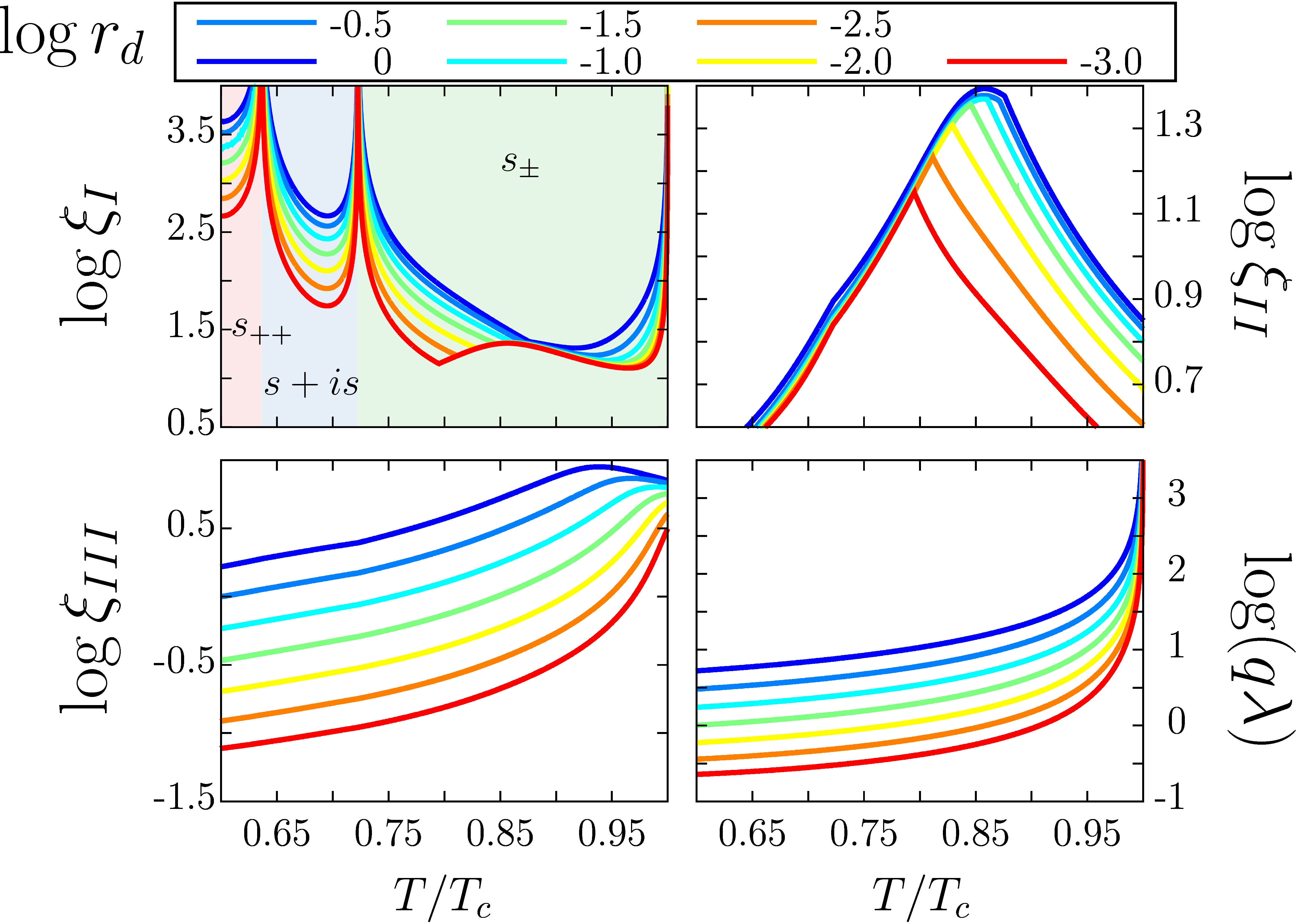
Figure 8: Effect of relative diffusion constant on the different length scales and on the upper critical field $\mathrm{H}_{c2}$ (corresponding to panel (B) of diagram Fig. 1). The top block displays the length scales as functions of the temperature for a given interband scattering $\Gamma=0.7275$ The relative diffusion constant affects only quantitatively the different length scales and do not affect the phase diagram. Similarly, the bottommost panel shows upper critical field $\mathrm{H}_{c2}$ as a function of the temperature for the same parameter set. Increasing the relative diffusion constant also increases the upper critical field.

Figure 8 shows the effect of the relative diffusion constant on the different length scales and on the upper critical field $\mathrm{H}_{c2}$, for a dirty two-band superconductor with nearly degenerate bands and intermediate repulsive interband pairing interaction (corresponding to panel (B) of diagram Fig. 1) . Relative diffusion constant has only a quantitative influence on the various length scales, while it increases the upper critical field $\mathrm{H}_{c2}$.

References

- Mazin et al. (2008) I. I. Mazin, D. J. Singh, M. D. Johannes, and M. H. Du, “Unconventional Superconductivity with a Sign Reversal in the Order Parameter of ,” Phys. Rev. Lett. 101, 057003 (2008).
- Chubukov et al. (2008) A. V. Chubukov, D. V. Efremov, and I. Eremin, “Magnetism, superconductivity, and pairing symmetry in iron-based superconductors,” Phys. Rev. B 78, 134512 (2008).
- Hirschfeld et al. (2011) P. J. Hirschfeld, M. M. Korshunov, and I. I. Mazin, “Gap symmetry and structure of Fe-based superconductors,” Reports on Progress in Physics 74, 124508 (2011).
- Efremov et al. (2011) D. V. Efremov, M. M. Korshunov, O. V. Dolgov, A. A. Golubov, and P. J. Hirschfeld, “Disorder-induced transition between and states in two-band superconductors,” Phys. Rev. B 84, 180512 (2011).
- Garaud et al. (2017) Julien Garaud, Mihail Silaev, and Egor Babaev, “Change of the vortex core structure in two-band superconductors at the impurity-scattering-driven crossover,” Phys. Rev. B 96, 140503 (2017).
- Garaud et al. (2018) Julien Garaud, Alberto Corticelli, Mihail Silaev, and Egor Babaev, “Field-induced coexistence of and superconducting states in dirty multiband superconductors,” Phys. Rev. B 97, 054520 (2018).
- Bobkov and Bobkova (2011) A. M. Bobkov and I. V. Bobkova, “Time-reversal symmetry breaking state near the surface of an superconductor,” Phys. Rev. B 84, 134527 (2011).
- Stanev and Koshelev (2014) Valentin Stanev and Alexei E. Koshelev, “Complex state induced by impurities in multiband superconductors,” Phys. Rev. B 89, 100505 (2014).
- Silaev et al. (2017) Mihail Silaev, Julien Garaud, and Egor Babaev, “Phase diagram of dirty two-band superconductors and observability of impurity-induced state,” Phys. Rev. B 95, 024517 (2017).
- Ng and Nagaosa (2009) T. K. Ng and N. Nagaosa, “Broken time-reversal symmetry in Josephson junction involving two-band superconductors,” Europhysics Letters 87, 17003–+ (2009).
- Stanev and Tešanović (2010) Valentin Stanev and Zlatko Tešanović, “Three-band superconductivity and the order parameter that breaks time-reversal symmetry,” Phys. Rev. B 81, 134522 (2010).
- Carlström et al. (2011a) Johan Carlström, Julien Garaud, and Egor Babaev, “Length scales, collective modes, and type-1.5 regimes in three-band superconductors,” Phys. Rev. B 84, 134518 (2011a).
- Maiti and Chubukov (2013) Saurabh Maiti and Andrey V. Chubukov, “ state with broken time-reversal symmetry in Fe-based superconductors,” Phys. Rev. B 87, 144511 (2013).
- Böker et al. (2017) Jakob Böker, Pavel A. Volkov, Konstantin B. Efetov, and Ilya Eremin, “ superconductivity with incipient bands: Doping dependence and STM signatures,” Phys. Rev. B 96, 014517 (2017).
- Silaev and Babaev (2011) Mihail Silaev and Egor Babaev, “Microscopic theory of type-1.5 superconductivity in multiband systems,” Phys. Rev. B 84, 094515 (2011).
- Gurevich (2003) A. Gurevich, “Enhancement of the upper critical field by nonmagnetic impurities in dirty two-gap superconductors,” Phys. Rev. B 67, 184515 (2003).
- Silaev and Babaev (2012) Mihail Silaev and Egor Babaev, “Microscopic derivation of two-component Ginzburg-Landau model and conditions of its applicability in two-band systems,” Phys. Rev. B 85, 134514 (2012).
- Babaev et al. (2002) Egor Babaev, L. D. Faddeev, and Antti J. Niemi, “Hidden symmetry and knot solitons in a charged two-condensate Bose system,” Phys. Rev. B 65, 100512 (2002).
- Babaev (2002) Egor Babaev, “Vortices carrying an arbitrary fraction of magnetic flux quantum in two-gap superconductors,” Phys. Rev. Lett. 89, 067001 (2002).
- Tinkham (1995) M. Tinkham, Introduction To Superconductivity (McGraw-Hill, 1995).
- Plischke and Bergersen (1989) Michael Plischke and Birger Bergersen, Equilibrium statistical physics (Prentice Hall Englewood Cliffs, N.J, 1989) pp. xi, 356 p. :.
- Svistunov et al. (2015) B.V. Svistunov, E.S. Babaev, and N.V. Prokof’ev, Superfluid States of Matter (Taylor & Francis, 2015).
- Gygi and Schlüter (1991) François Gygi and Michael Schlüter, “Self-consistent electronic structure of a vortex line in a type-II superconductor,” Phys. Rev. B 43, 7609–7621 (1991).
- Carlström et al. (2011b) Johan Carlström, Egor Babaev, and Martin Speight, “Type-1.5 superconductivity in multiband systems: Effects of interband couplings,” Phys. Rev. B 83, 174509 (2011b).
- Leggett (1966) A. J. Leggett, “Number-Phase Fluctuations in Two-Band Superconductors,” Progress of Theoretical Physics 36, 901–930 (1966).
- Stanev (2012) Valentin Stanev, “Model of collective modes in three-band superconductors with repulsive interband interactions,” Phys. Rev. B 85, 174520 (2012).
- Marciani et al. (2013) M. Marciani, L. Fanfarillo, C. Castellani, and L. Benfatto, “Leggett modes in iron-based superconductors as a probe of time-reversal symmetry breaking,” Phys. Rev. B 88, 214508 (2013).
- Blumberg et al. (2007) G. Blumberg, A. Mialitsin, B. S. Dennis, M. V. Klein, N. D. Zhigadlo, and J. Karpinski, “Observation of Leggett’s Collective Mode in a Multiband MgB2 Superconductor,” Phys. Rev. Lett. 99, 227002 (2007).
- Garaud et al. (2016a) Julien Garaud, Mihail Silaev, and Egor Babaev, “Thermoelectric Signatures of Time-Reversal Symmetry Breaking States in Multiband Superconductors,” Phys. Rev. Lett. 116, 097002 (2016a).
- Silaev et al. (2015) Mihail Silaev, Julien Garaud, and Egor Babaev, “Unconventional thermoelectric effect in superconductors that break time-reversal symmetry,” Phys. Rev. B 92, 174510 (2015).
- Silaev and Babaev (2013) Mihail Silaev and Egor Babaev, “Unusual mechanism of vortex viscosity generated by mixed normal modes in superconductors with broken time reversal symmetry,” Phys. Rev. B 88, 220504 (2013).
- Lin et al. (2016) Shi-Zeng Lin, Saurabh Maiti, and Andrey Chubukov, “Distinguishing between and pairing symmetries in multiband superconductors through spontaneous magnetization pattern induced by a defect,” Phys. Rev. B 94, 064519 (2016).
- Maiti et al. (2015) Saurabh Maiti, Manfred Sigrist, and Andrey Chubukov, “Spontaneous currents in a superconductor with symmetry,” Phys. Rev. B 91, 161102 (2015).
- Hecht (2012) F. Hecht, “New development in Freefem++,” J. Numer. Math. 20, 251–265 (2012).
- Garaud et al. (2016b) Julien Garaud, Egor Babaev, Troels Arnfred Bojesen, and Asle Sudbø, “Lattices of double-quanta vortices and chirality inversion in superconductors,” Phys. Rev. B 94, 104509 (2016b).
- Moshchalkov et al. (2009) Victor Moshchalkov, Mariela Menghini, T. Nishio, Q. H. Chen, A. V. Silhanek, V. H. Dao, L. F. Chibotaru, N. D. Zhigadlo, and J. Karpinski, “Type-1.5 Superconductivity,” Phys. Rev. Lett. 102, 117001 (2009).
- Babaev and Speight (2005) Egor Babaev and Martin Speight, “Semi-Meissner state and neither type-I nor type-II superconductivity in multicomponent superconductors,” Phys. Rev. B 72, 180502 (2005).
- Babaev et al. (2010) E. Babaev, J. Carlström, and M. Speight, “Type-1.5 Superconducting State from an Intrinsic Proximity Effect in Two-Band Superconductors,” Phys. Rev. Lett. 105, 067003–+ (2010).
- Sethna (2006) James P. Sethna, Statistical Mechanics: Entropy, Order Parameters and Complexity (Oxford Master Series in Physics), illustrated edition ed. (Oxford University Press, 2006).
- Ray et al. (2014) S. J. Ray, A. S. Gibbs, S. J. Bending, P. J. Curran, E. Babaev, C. Baines, A. P. Mackenzie, and S. L. Lee, “Muon-spin rotation measurements of the vortex state in Sr2RuO4: Type-1.5 superconductivity, vortex clustering, and a crossover from a triangular to a square vortex lattice,” Phys. Rev. B 89, 094504 (2014).
- Garaud and Babaev (2014) Julien Garaud and Egor Babaev, “Domain Walls and Their Experimental Signatures in Superconductors,” Phys. Rev. Lett. 112, 017003 (2014).
- Vadimov and Silaev (2018) V. L. Vadimov and M. A. Silaev, “Polarization of spontaneous magnetic field and magnetic fluctuations in anisotropic multiband superconductors,” ArXiv e-prints (2018), arXiv:1804.10281 [cond-mat.supr-con] .
- Grinenko et al. (2017) V. Grinenko, P. Materne, R. Sarkar, H. Luetkens, K. Kihou, C. H. Lee, S. Akhmadaliev, D. V. Efremov, S.-L. Drechsler, and H.-H. Klauss, “Superconductivity with broken time-reversal symmetry in ion-irradiated Ba0.27K0.73Fe2As2 single crystals,” Phys. Rev. B 95, 214511 (2017).