Observational constraints on the free parameters of an interacting Bose-Einstein gas as a dark-energy model
Abstract
Dark energy is modelled by a Bose-Einstein gas of particles with an attractive interaction. It is coupled to cold dark matter, within a flat universe, for the late-expansion description, producing variations in particle-number densities. The model’s parameters, and physical association, are: , , the dark-energy rest-mass energy density and the dark-matter term scaling as a mass term, respectively; , the self-interaction intensity; , the energy exchange rate. Energy conservation relates such parameters. The Hubble equation omits , but also contains , the present-day expansion rate of the flat Friedman-Lemâitre-Robertson-Walker metric, and , the baryon energy density, used as a prior. This results in the four effective chosen parameters , , , , fit with the Hubble expansion rate , and data from its value today, near distance, and supernovas. We derive wide and likelihood regions compatible with definite positive total CDM and IBEG mass terms. Additionally, the best-fit value of parameter relieves the coincidence problem, and a second potential coincidence problem related to the choice of .
1 Introduction
The observed accelerated expansion of the Universe suggests that the source with the greatest contribution to the total energy density of the homogeneous Friedman-Lemaître-Robertson-Walker (FLRW) metric is an unknown form of energy with negative pressure called dark energy (DE)[1]. The second source with the greatest contribution is pressureless cold dark matter (CDM), followed by ordinary (baryonic) matter. Both dark sources presumably only interact with ordinary matter and radiation through gravitation, but it is reasonable to assume that there is an interaction between the dark sources, as it avoids or relieves the coincidence problem [2], associated to DE as a cosmological constant/scalar field. In addition, galaxy-cluster dynamics data[3] and the integrated Sachs-Wolfe effect[4] support the idea of an interacting dark energy (IDE). Several IDE models exist in the literature, as those motivated by particle physics, thermodynamics, and phenomenological assumptions[5, 6, 7].
The non-relativistic Bose-Einstein gas (IBEG) model, applied to the late universe, is an example of an IDE with a detailed microscopic description. Its attractive interaction component between the particles generates a negative pressure. In an application to the early universe[8], it leads to an accelerated expansion under certain conditions. Including a general energy-exchange mechanism, the IBEG explains the present accelerated expansion of the Universe, and avoids (or greatly relieves) the coincidence problem. The background dynamics of the IBEG model is similar to that of the CDM model for certain free-parameter choices [2].
Observational data can constrain the free parameters of the DE models by means of Bayesian methods[9]. Several IDE models have been tested in the literature, e.g.,[10, 11, 12]. Some observational data are model independent such as the local Hubble constant measurements[13, 14], the data from the history of the Hubble constant obtained by the cosmic chronometer approach[15, 16, 17, 18] or the type Ia supernova[19, 20]. Other data sets are model dependent, as the anisotropy of cosmic microwave background measurements[21, 1], the baryonic acoustic oscillation (BAO) data[22], the gas mass fraction[23], and the evolution of the growth function[24]. In this paper we find bounds on the free parameters of the IBEG model by means of observational data that is model independent. Additionally, we compare the observational bounds with other constraints of theoretical origin. This kind of analysis is of vital importance to the IBEG model given the physical nature and detailed information of the free parameters.
The paper is organized as follows. In section 2, we review the IBEG model of late accelerated expansion, defining the corresponding Hubble constant . In section 3, we obtain the observational constraints on the model’s free parameters by means of Bayesian methods. The observational data sets we use are the local Hubble constant measurements, and the Hubble-parameter history data, including type Ia supernova luminosity-distance data. In section 4, we compare the observational constraints with theoretical bounds. Finally, in section 5, we summarize the work. From now on, we assume units for which . As usual, a zero subindex refers to a variable’s present value; likewise, we normalize the present day FLRW metric scale factor by setting .
2 Interacting Bose-Einstein gas as dark energy
The IBEG model consists of a Bose-Einstein gas of spin-zero non-relativistic particles interacting through an attractive contact local potential between particle pairs. The quasiparticle energy is composed of a kinetic and a potential-energy terms, and this feature is maintained for the total energy, where the kinetic contribution is independent of the particle number (see [8, 2] for a detailed model description). If the IBEG is set at a temperature below the critical one , particles start becoming condensate, with accounting the condensate number density, and , , the non-condensate and total number densities, respectively. The gas energy density then reads [8]
| (1) |
where is the IBEG particle mass, providing the energy density at rest, , for spin-zero particles and is related to the kinetic energy term of the gas, and is a negatively-defined potential term that accounts for the interaction between the particles. The gas pressure can be obtained from its description in the thermodynamical limit and, using , taking the form
| (2) |
where .
Although the IBEG gas by itself can be used in a early acceleration cosmological scenario [8], it is necessary to assume that it is coupled to CDM and that the number density is not constant in order to obtain a late acceleration solution in a FLRW frame[2]. In this case, the model is defined in an expanding flat FLRW metric as
where is the scale factor and , and are the time, the radius and solid-angle comoving coordinates of the metric, respectively. The energy-momentum source is composed of pressureless baryonic matter with energy density , pressureless cold dark matter (CDM) with energy density (Ref. [2] uses for ,) and the IBEG with energy density given by eq. (1). The latter two sources are coupled in such a way that the IBEG non-condensate number density is changed as a Markoff’s process following the phenomenological law
| (3) |
where and are the free parameters that model the coupling, and is assumed (as the influence of the first component diminishes as increases).
Note that the IBEG particles created by the coupling are non-condensated and, additionally, no further condensation occurs at that epoch as scales as (see [2] for details). Consequently, it is reasonable to set the IBEG condensate particle number density to null, and, then, . The energy-density conservation equation for the three sources read
| (4) | |||
| (5) | |||
| (6) |
where the dot means derivation with respect to time, is the coupling term. This system is completed with the Hubble equation .
Using (1,2) and from the derivation of (3), the coupling term can be obtained
| (7) |
where we have defined the parameters
| (8) |
(Ref. [2] uses for ).
Consequently, the three-source energy densities evolve as
| (9) | |||||
| (10) | |||||
| (11) |
where is the baryonic matter present-day energy density, and is a present-day CDM term that evolves as a mass term (i.e., the CDM energy-density component that scales as ).
The case should be treated apart. Then, the non-condensate particle number evolves proportionally to the volume and scales as in a FLRW scenario. Consequently, the IBEG energy density is constant, as the term in the CDM model. Similarly, the IBEG pressure is constant with , so the coupling term is not null but reads
| (12) |
while the CDM in our model evolves as
| (13) |
In such aspects, we safely conclude that the IBEG-model dynamics differs from that of the CDM model in the case.
We note that the present-day CDM total energy density is
| (14) |
The free parameters of the IBEG model are then , , , , and .
The Hubble equation for can be rewritten in terms of the redshift as
| (15) |
where is the present-day Hubble constant, and we have defined with . The above Hubble constant does not depend on the free parameter . A relation between the free parameters can be obtained from Eq. (15) evaluated at
| (16) |
and, from (15) and (16), it is possible to rewrite the equation for as
where is given in units of and replaces as a free parameter of the model. Regarding the case again, we point at similarities of the IBEG and CDM models in ; given the above definition, for the Hubble factor is formally identical for both models. Using Hubble-factor related data in the case would make the parameters and indistinguishable for the fit, with the combination playing an identical role as the term.
The validity of the model’s free parameters was discussed in [2], and the analysis used the total CDM energy density and the total IBEG energy density , fixed with CDM model best-fit values ( and of the total energy density of the Universe, respectively). Additionally, the Hubble expansion rate was set at , based on supernova data. These values were set in order to compare the IBEG and CDM models. On the other hand, in this work, no such parameters are fixed beforehand and the model’s validity is discussed as well.
The observational data directly related to the Hubble constant with (as the data of the local value of the Hubble constant, the history of Hubble constant data and the type IA supernova data) can be used to constrain the free parameters , and directly. Parameters and have both the same dependence on , so they cannot be constrained separately by Hubble-constant related observations, unless some priors are used. On the other hand, no information on can be obtained directly from the Bayesian analysis of this kind of data, as it is absent from the Hubble expansion rate expression (2).
3 Constraints on the IBEG-model free parameters by the Hubble constant
In order to constrain the model’s free parameters, we use the Bayesian approach and Monte Carlo Markov Chains (MCMC) integrated within the code SimpleMC[25] developed by A. Slosar and J. Vazquez for[26].
We define
| (17) |
for a given set of uncorrelated data (sud) consisting of points of the type , and corresponding to a theoretical function of the type ( being a list of free parameters of a given model,) where is the error of the data point . The choice of free-parameter values that minimize has the largest probability to be true, given the sud [9], and we refer to them as the best-fit parameter values .
We also derive the parameter-space confidence regions: the likelihood is the parameter-space region around the best-fit value for which any choice of has a probability for the sud be measured; and the likelihood parameter-space region has a probability. These regions are used to constrain the model’s free parameters.
In order to evaluate the fit quality of the best-fit parameter values, it is possible to define the degrees of freedom (dof) of a given sud as the number of data points minus the number of free parameters and, then, to compute . The theoretical function with the best-fit parameter values poorly fits the given sud when , while of order of unity represents a good fit [9]. We also can compare the fit quality of with other theories by comparing the corresponding .
In this section we consider three sud related to . Given that cannot be determined with this kind of data, and that it is not directly related to the IBEG model, we will set it as a Gaussian prior with mean value , and standard deviation , values reported in[27] from primordial-deuterium abundance. For the rest of the free parameters, we assume a range used as a prior by the MCMC as well. is assumed in[2], so we use the range in the MCMC. is related to the CDM mass-like term of the energy density, so it is defined positive and in the range . is related to and is defined in the range . We note that both and are not total energy-density terms and they should not be constrained beforehand to be smaller than unity, as the parameters of the CDM model. Finally, is taken in the range , as it is related to the of the Hubble-constant local value .
We proceed to obtain the constraints on the free parameters , , and .
3.1 Constraints from local value of the Hubble constant data: Gaussian priors
A local measurement of the Hubble constant was reported from the Hubble Space Telescope (HST) data with a 2.4% precision in[13]. The obtained value is . We use it as a Gaussian prior to obtain a first parameter constraint. The result is given in table 2 and the and contours can be appreciated in figure 1.
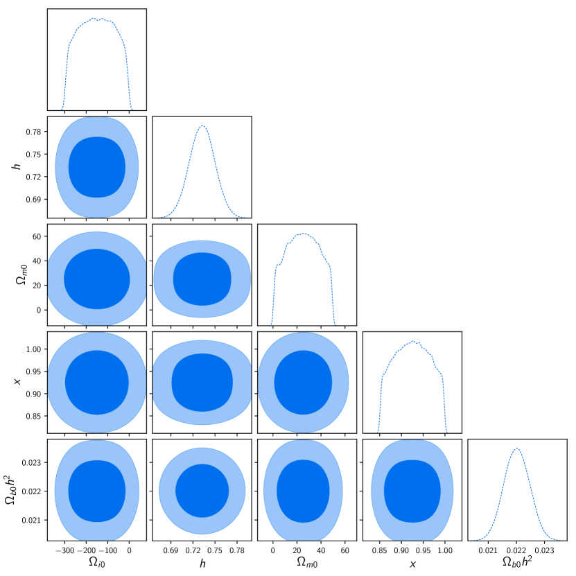
An independent measurement of the local Hubble constant was recently obtained by the gravitational wave (GW) detectors LIGO and Virgo, jointly with the 1M2H, the Dark Energy Camera GW-EM, DES, DLT40, Las Cumbres Observatory, VINROUGE, and MASTER Collaborations [14]. They measured it both in the GW spectrum and in the electromagnetic spectrum, from the merger of a binary neutron-star system. The value obtained is , which is compatible with the other measurement considered above to . We proceed as previously, setting a Gaussian prior to with mean value and standard deviation . The IBEG free-parameter constraints are presented in table 2 under the tag GW. Given that both values considered in this section are compatible to , the IBEG free-parameter contours observed are almost identical, with the exception of .
There are other local Hubble-constant estimates including cosmic microwave background (CMB) measurements from Planck[1] (), and Barionic Acoustic Oscillation (BAO) measurements from SDSS30, strong lensing measurements from H0LiCOW31, and high-angular-multipole CMB measurements from SPT32. All of them are model dependent via the linear-perturbation evolution and the background dynamics. We decided not to consider them as we restrict ourselves to measurements related to the background dynamics of the model.
3.2 Constraints from history of the Hubble-constant data
We next consider observational data on the Hubble-constant history, , represented in table 1 with their respective uncertainties and sources in the literature. The data from[15, 16, 17, 18] are obtained by the cosmic-chronometer approach and are model independent. The remaining data are related to BAO observations that can be model dependent. In this case and given the large uncertainties in the measurements, we assume that the deviation of the acoustic peak and distance scale of the IBEG model will not be very different from that of the CDM model, and thus, the corresponding data can be used as well.
| ref. | ref. | ||||||
|---|---|---|---|---|---|---|---|
| 0.07 | 69.0 | 19.16 | [28] | 0.570 | 100.3 | 3.7 | [29] |
| 0.09 | 69.0 | 12 | [30] | 0.593 | 104 | 13 | [15] |
| 0.12 | 68.6 | 26.2 | [28] | 0.6 | 87.9 | 6.1 | [31] |
| 0.17 | 83 | 8 | [30] | 0.680 | 92 | 8 | [15] |
| 0.179 | 75 | 4 | [15] | 0.730 | 97.3 | 7 | [31] |
| 0.199 | 75 | 5 | [15] | 0.781 | 105 | 12 | [15] |
| 0.2 | 72.9 | 29.6 | [28] | 0.875 | 125 | 17 | [15] |
| 0.27 | 77 | 14 | [30] | 0.88 | 90 | 40 | [16] |
| 0.28 | 88.8 | 36.6 | [28] | 0.9 | 117 | 23 | [30] |
| 0.32 | 79.2 | 5.6 | [29] | 1.037 | 154 | 20 | [15] |
| 0.352 | 83 | 14 | [15] | 1.3 | 168 | 17 | [30] |
| 0.3802 | 83 | 13.5 | [17] | 1.363 | 160 | 33.6 | [18] |
| 0.4 | 95 | 17 | [30] | 1.43 | 177 | 18 | [30] |
| 0.4004 | 77 | 10.2 | [17] | 1.53 | 140 | 14 | [30] |
| 0.4247 | 87.1 | 11.2 | [17] | 1.75 | 202 | 40 | [30] |
| 0.44 | 82.6 | 7.8 | [31] | 1.965 | 186.5 | 50.4 | [18] |
| 0.44497 | 92.8 | 12.9 | [17] | 2.34 | 222 | 7 | [32] |
| 0.4783 | 80.9 | 9 | [17] | 2.36 | 226 | 8 | [33] |
| 0.480 | 97 | 62 | [16] |
The constraints on the free parameters from the data can be found in table 2 and the likelihood is represented in figure 2. The parameter is poorly constricted by this sud, as can be appreciated in 2.
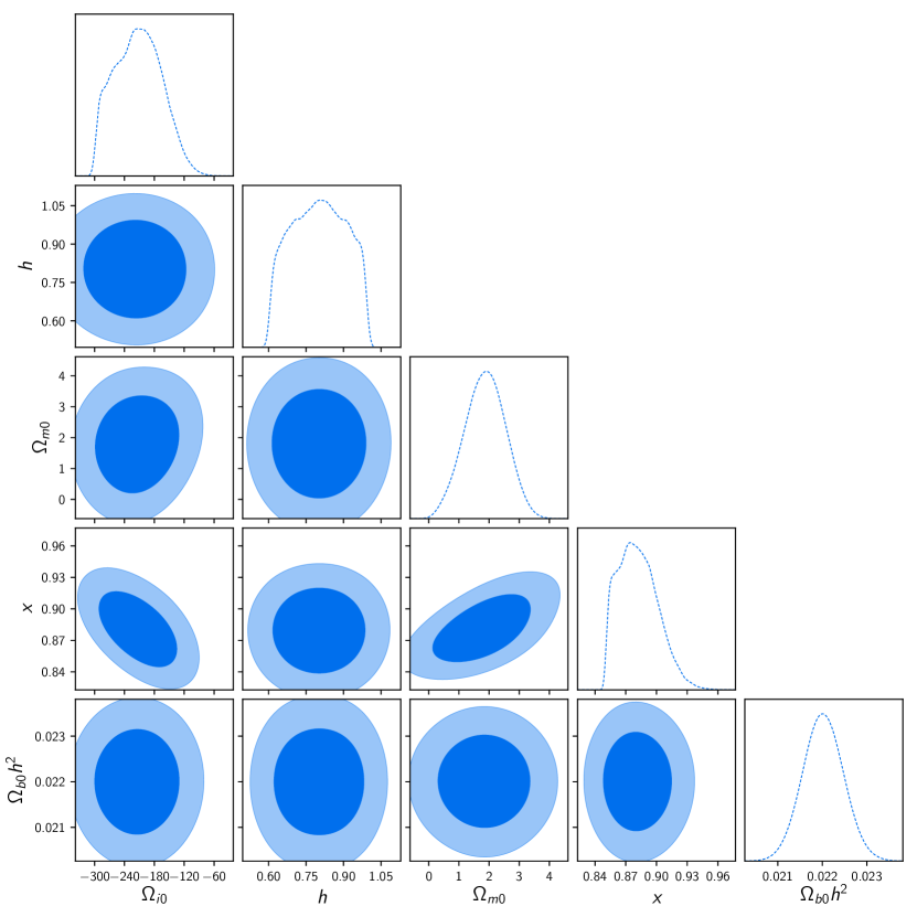
For this sud, the dof and, consequently, which can be interpreted as the model slightly ’over-fitting’ the data. It is possible to use the data with the CDM model implemented on the SimpleMC code, and then, ( can be interpreted as the model has not fully captured the data). In this sense, we can only conclude that both the IBEG and CDM present a similar fit quality of the data, as both have values close to .
A comparison between the fit of both models can also be made by means of the Akaike Information Criterion (AIC) and the Bayesian Information Criterion (BIC) [34, 35]. The first parameter is defined
| (18) |
where is the model’s number of free parameters. For this sud in the CDM case, the parameter is easily computed, , while for the IBEG model it is . The observational data suggest that the ”preferred model” corresponds to that with the smaller AIC parameter. The difference is interpreted as strong evidence against the CDM model. Another criterion is defined by means of the parameter
| (19) |
where for this sud. Then, and , and the difference is , which indicates strong evidence against the CDM in comparison to the IBEG model.
3.3 Constraints from Supernova type Ia data.
The type Ia supernova distance modulus () data is the more constrained model-independent data considered in this work. The distance modulus is directly related to as
To get likelihoods of the IBEG parameters from this sud we use the joint light curves (JLA) from [36] and a different definition of the , given that the data is used in 30 correlated bins. In this case,
| (20) |
where is the term of the reported correlation matrix.
The results of the analysis are found in table 2, and the likelihood regions in figure 3. The region of is more restricted from the JLA data than it is in the rest of the data sets. On the other hand, the region of the same parameter is still similar to the other data sets.
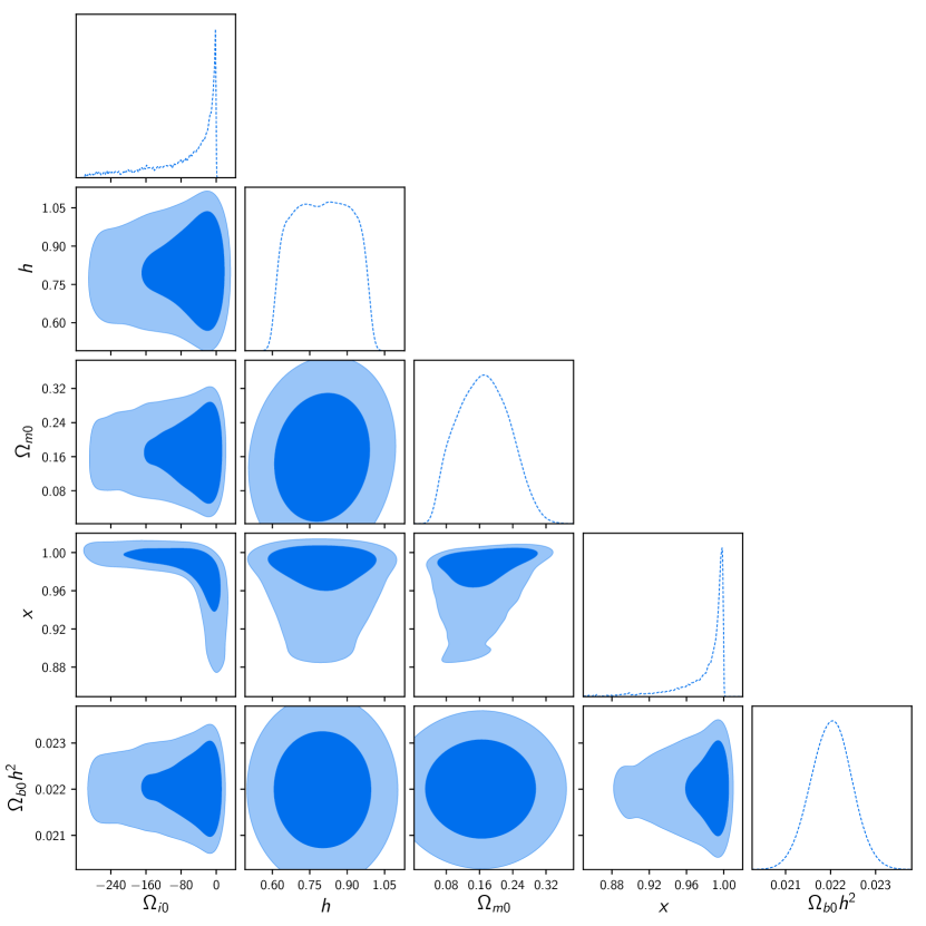
The dof in this case is and the corresponding , which can be interpreted as a good fit of the data. The CDM model reads , and we can conclude that both models have an almost identical fit quality.
As in subsection 3.2, we compare both models for this sud by means of the AIC and BIC parameters. The AIC parameter of both models is and , respectively. The difference between them reads which can be interpreted as ”slight evidence in favor” of the IBEG model. The parameter and with a difference as is interpreted as ”evidence against” the IBEG model. For this sud, both criteria present a tension, which can be explained due to the larger parameter number of the IBEG model (BIC strongly penalizes the parameter number) [34, 35]. The tension between AIC and BIC criteria has been reported as well for the CDM model and several interacting DE models [37].
3.4 Constraints combining three sets of data: HSTJLA.
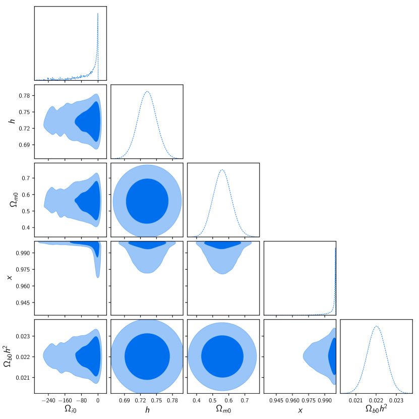
We define to obtain a total likelihood combining the three sets of model-independent observations and run the MCMC implemented in SimpleMC to explore the free-parameter space. For the present-day Hubble parameter, we consider the Gaussian prior HST motivated, on one hand, by the fact that it is the observation of present-day Hubble parameter with the smaller error, and, on the other hand, by the fact that the GW observation is compatible with it. The total constraints and likelihoods of the free parameters are shown in table 2 and figure 4, respectively.
| HST | GW | |||||
|---|---|---|---|---|---|---|
| Param. | Value | Value | Value | |||
| 14.11 | 14.16 | 47.70 | 14.07 | 3.35 | 0.95 | |
| 0.022 | 1 | 0.021 | 1 | 0.022 | 1 | |
| 0.73 | 0.02 | 0.68 | 0.03 | 0.66 | 0.10 | |
| 74.72 | 47.15 | -247.65 | 57.89 | 233.12 | 65.75 | |
| 0.92 | 0.04 | 0.85 | 0.04 | 0.92 | 0.03 | |
| JLA | HST++JLA | |||
|---|---|---|---|---|
| Param. | Value | Value | ||
| 0.10 | 0.07 | 0.52 | 0.08 | |
| 0.023 | 3.0 | 0.022 | 2.0 | |
| 0.62 | 0.05 | 0.70 | 0.02 | |
| 23.77 | 27.05 | 3.60 | 12.38 | |
| 0.98 | 0.02 | 0.97 | 0.01 | |
4 Implications of the observational constraints on the IBEG model
Next, we compare the observational bounds with theoretical considerations, e.g., that the IBEG energy-density mass term be positive definite. Given the detailed physical description of the free parameters, the observational constraints could be incompatible with physical bounds, and the IBEG model could be discarded. Other theoretical demands about the IBEG model are preferable but not compulsory, e.g., that the IBEG model solve or alleviate the coincidence problem.
Most parameters that characterize the IBEG model are constrained and lead to the best-fit values from observations: ; , where is related to the rest of the parameters by eq. (16). However, the model-independent observations related to the Hubble constant, such as , or JLA , cannot give direct information about . Also, the parameters that define the microscopic nature of the IBEG cannot be obtained with the above observables (the IBEG particle mass , the non-condensate state particle number today, , and finally, the self-interaction coupling .) The CDM energy density today is also unknown. On the other hand, the energy-exchange term is constrained by observations to the best-fit value of . As stated in[2], greatly relieves the coincidence problem in comparison to the CDM model as varies at a slow rate compared with the rate of expansion . In fact, solves the coincidence problem. As is compatible to with the observations, we conclude that its allowed values constrain the IBEG energy-exchange term in a way that they solve the coincidence problem.
Given that is the IBEG mass term, it is positive definite. The parallelism of the IBEG and CDM models, and observations suggest that , with defined in (14) is also positive, (or, at worst, null.) Then, using the relation (16), we put the bound over the free parameters
| (21) | |||||
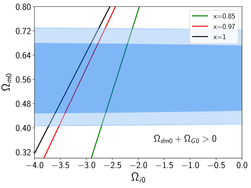
Although the best-fit values for such parameters, reported in table 2 from the HSTJLA case, is incompatible with condition (21), there is a wide and region of compatible likelihoods.
Figure 5 shows the bound over the parameters given by (21) for , , and three different choices of in the space, for the , where the space on the right-hand side of the line represents parameter choices with . The lines correspond to: and , respectively the upper and lower values considered for parameter in the IBEG model[2]. Finally, is the best-fit value from the HSTJLA analysis. In the same plot, we show the and likelihoods from the HSTJLA analysis. We conclude that the IBEG model is consistent with condition 21.
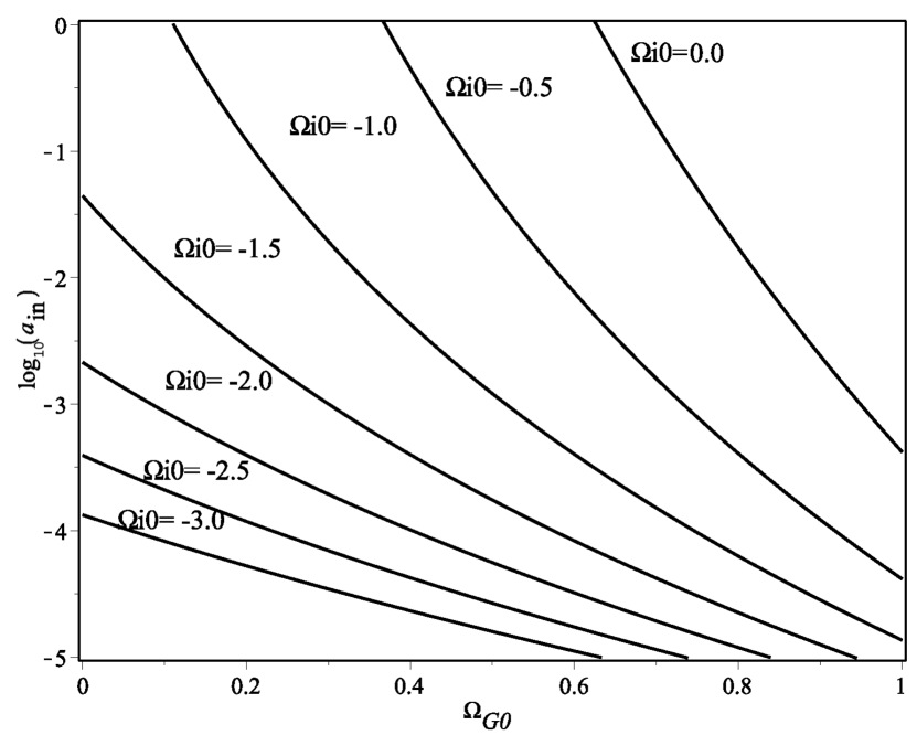
Another, non-compulsory demand for the IBEG model is that for some free-parameter choices and scale factor in the past. In[2], describes the moment when the CDM-IBEG energy interchange starts.
If is near today’s value , a second coincidence problem arises, as the acceleration-producing substance exists only in the near past. Given that is not determined by the observations, it is not possible to limit from this work, but assuming the likelihood contours obtained by the data analysis, there is a wide range of choices that leads to an smaller enough than . Figure 6 shows for , , and different , in the region with . For any chosen , there is a wide region of for which is smaller enough than , or even smaller than . Similar plots can be obtained for different inside the likelihood region of figure 5. Despite the lack of information on , we conclude that the coincidence problem associated to can be avoided for parameter choices in the allowed region of figure 5, for .
5 Conclusions
The IBEG model consists of a flat FLRW metric containing baryonic, CDM, and IBEG sources, the latter for DE. The CDM, IBEG components exchange energy at a rate compatible with a Markoff’s process. The IBEG particles’ attractive self-interaction produces negative presure responsible for an accelerated expansion of the metric[2], mimicking the CDM-model dynamics. The IBEG model parameters have a direct physical meaning, and any additional bound on them produces information on its constituents. For certain parameter choices, the IBEG model solves or alleviates the coincidence problem, and a second related problem, as consistent energy-exchange starts can be found in the past. This effect is also consistent with the application of the model to the early universe[8], which avoids the energy-exchange component then.
Observational data on the background dynamics from the Hubble parameter constrain the IBEG-model’s free parameters. By setting limits on their range and comparing with physical requirements, one may maintain or discard the model. The data used in this work are: the local measurements of the Hubble constant [13, 14], the history of [28]-[33], and the modulus distance of type Ia supernova in the joint light curves (JLA) from [36]. A Gaussian prior is used on the baryonic energy density based on universe measured values [27].
The data strongly bound the parameter , related to the IBEG energy-exchange rate, finding the best fit , which relieves the coincidence problem in the IBEG model. The and likelihoods for the parameters related to CDM mass energy density () and the IBEG self-interaction () are wide, not too restrictive, and compatible with the theoretical and observational condition . The data bounds are also compatible with parameter choices not affected by the second coincidence problem related to the time when the IBEG-CDM energy exchange starts, defined in terms of the scale factor . In this sense, we can conclude that the IBEG model remains consistent with the observational data used in this work and Bayesian analysis, which restrict the IBEG-model free parameter space, relieving the traditional and decay-start coincidence problems. The AIC and BIC parameters computed for the history of data tend to favor the IBEG model compared to the CDM model. On the other hand, the JLA data present a tension between both criteria, AIC parameters favoring the IBEG model while BIC one favoring the CDM model. Such a tension is present in other DE models (such as the CDM or some interacting DE models), and can be explained in terms of the larger free-parameter number of the latter [37]. In general, we conclude that the IBEG model is favoured by the observational data, in the same way as other interacting DE data recently studied in the literature [7, 37, 38, 39].
Finally, the IBEG particle mass-related parameter cannot be bounded by the kind of data used in this work. Other observational data, related to the linear perturbation evolution of the model considered, can constrain it. Those model-related observations include the CMB anisotropy measurements[21, 1], the BAO data[22], the gas-mass fraction[23], the evolution of the growth function[24]. These data are being analyzed and will be presented in a future work.
Acknowledgments
The authors acknowledge financial support from DGAPA-UNAM, project IN112916.
References
References
- [1] Ade P A, Aghanim N, Arnaud M, Ashdown M, Aumont J, Baccigalupi C, Banday A, Barreiro R, Bartlett J, Bartolo N et al. 2016 Astronomy & Astrophysics 594 A13
- [2] Besprosvany J and Izquierdo G 2015 Classical and Quantum Gravity 32 055015
- [3] Abdalla E, Abramo L R, Sodré L and Wang B 2009 Physics Letters B 673 107-110
- [4] Olivares G, Atrio-Barandela F and Pavón D 2008 Physical Review D 77 103520
- [5] Copeland E J, Sami M and Tsujikawa S 2006 International Journal of Modern Physics D 15 1753-1935
- [6] Bamba K, Capozziello S, Nojiri S and Odintsov S D 2012 Astrophysics and Space Science 342 155-228 ISSN 1572-946X
- [7] Wang B, Abdalla E, Atrio-Barandela F and Pavón D 2016 Reports on Progress in Physics 79 096901
- [8] Izquierdo G and Besprosvany J 2010 Classical and Quantum Gravity 27 065012
- [9] Verde L 2010 Statistical methods in cosmology Lectures on Cosmology (Springer) pp 147-177
- [10] Durán I, Pavón D and Zimdahl W 2010 Journal of Cosmology and Astroparticle Physics 2010 018
- [11] Ferreira P C and Pavón D 2016 Universe 2 27
- [12] Yang W, Banerjee N and Pan S 2017 arXiv preprint arXiv:1705.09278
- [13] Riess A G, Macri L M, Hoffmann S L, Scolnic D, Casertano S, Filippenko A V, Tucker B E, Reid M J, Jones D O, Silverman J M et al. 2016 The Astrophysical Journal 826 56
- [14] Abbott, T. D. et al., The LIGO Scientific Collaboration et al. et al. 2017 Nature 551 85-88
- [15] Moresco M, Cimatti A, Jimenez R, Pozzetti L, Zamorani G, Bolzonella M, Dunlop J, Lamareille F, Mignoli M, Pearce H et al. 2012 Journal of Cosmology and Astroparticle Physics 2012 006
- [16] Stern D, Jimenez R, Verde L, Kamionkowski M and Stanford S A 2010 Journal of Cosmology and Astroparticle Physics 2010 008
- [17] Moresco M, Pozzetti L, Cimatti A, Jimenez R, Maraston C, Verde L, Thomas D, Citro A, Tojeiro R and Wilkinson D 2016 Journal of Cosmology and Astroparticle Physics 2016 014
- [18] Moresco M 2015 Monthly Notices of the Royal Astronomical Society: Letters 450 L16-L20
- [19] Riess A G, Filippenko A V, Challis P, Clocchiatti A, Diercks A, Garnavich P M, Gilliland R L, Hogan C J, Jha S, Kirshner R P et al. 1998 The Astronomical Journal 116 1009
- [20] Perlmutter S, Aldering G, Goldhaber G, Knop R, Nugent P, Castro P, Deustua S, Fabbro S, Goobar A, Groom D et al. 1999 The Astrophysical Journal 517 565
- [21] Spergel D N, Bean R, Doré O, Nolta M, Bennett C, Dunkley J, Hinshaw G, Jarosik N e, Komatsu E, Page L et al. 2007 The Astrophysical Journal Supplement Series 170 377
- [22] III SDSS 2017 Boss: Dark energy and the geometry of space http://www.sdss3.org/surveys/boss.php
- [23] Allen S, Rapetti D, Schmidt R, Ebeling H, Morris R and Fabian A 2008 Monthly Notices of the Royal Astronomical Society 383 879-896
- [24] Gong Y et al. 2008 Physical Review D 78 123010
- [25] Slosar A and Vazquez J 2017 Simplemc https://github.com/slosar/april
- [26] Vazquez J, Collaboration B et al. 2015 Cosmological implications of baryon acoustic oscillation (BAO) measurements APS April Meeting Abstracts
- [27] Cooke R J, Pettini M, Jorgenson R A, Murphy M T and Steidel C C 2014 The Astrophysical Journal 781 31
- [28] Zhang C, Zhang H, Yuan S, Liu S, Zhang T J and Sun Y C 2014 Research in Astronomy and Astrophysics 14 1221
- [29] Cuesta A J, Vargas-Magaña M, Beutler F, Bolton A S, Brownstein J R, Eisenstein D J, Gil-Marín H, Ho S, McBride C K, Maraston C et al. 2016 Monthly Notices of the Royal Astronomical Society 457 1770-1785
- [30] Simon J, Verde L and Jimenez R 2005 Physical Review D 71 123001
- [31] Blake C, Brough S, Colless M, Contreras C, Couch W, Croom S, Croton D, Davis T M, Drinkwater M J, Forster K et al. 2012 Monthly Notices of the Royal Astronomical Society 425 405-414
- [32] Delubac T, Bautista J E, Rich J, Kirkby D, Bailey S, Font-Ribera A, Slosar A, Lee K G, Pieri M M, Hamilton J C et al. 2015 Astronomy & Astrophysics 574 A59
- [33] Font-Ribera A, Kirkby D, Miralda-Escudé J, Ross N P, Slosar A, Rich J, Aubourg É, Bailey S, Bhardwaj V, Bautista J et al. 2014 Journal of Cosmology and Astroparticle Physics 2014 027
- [34] A. R. Liddle, 2004 Mon. Not. R. Astron. Soc. 351, L49
- [35] A. R. Liddle, 2007 Mon. Not. R. Astron. Soc. 377, L74
- [36] Betoule M, Kessler R, Guy J, Mosher J, Hardin D, Biswas R, Astier P, El-Hage P, Konig M, Kuhlmann S et al. 2014 Astronomy & Astrophysics 568 A22
- [37] Arevalo F, Cid A, Moya J, 2017 The European Physical Journal C 77 565
- [38] Nunes R, Pan S, Saridakis M 2016 Phys. Rev. D 94 023508
- [39] Xia D, Wang S 2016 Mon. Not. R. Astron. Soc. 463 no.1, 952