Asymptotic Distribution of
Parameters in Random Maps

Abstract.

We consider random rooted maps without regard to their genus, with fixed large number of edges, and address the problem of limiting distributions for six different parameters: vertices, leaves, loops, root edges, root isthmus, and root vertex degree. Each of these leads to a different limiting distribution, varying from (discrete) geometric and Poisson distributions to different continuous ones: Beta, normal, uniform, and an unusual distribution whose moments are characterised by a recursive triangular array.

Key words and phrases.

1. Introduction

1.1. Motivation for our work

Rooted maps form a ubiquitous family of combinatorial objects, of considerable importance in combinatorics, in theoretical physics, and in image processing. They describe the possible ways to embed graphs into compact oriented surfaces [LZ04].

The present paper focuses on asymptotic enumeration of basic parameters in rooted maps with no restriction on genus. From a generating function viewpoint, if the genus of the maps is not fixed, then the generating function of rooted maps is non-analytic (namely, convergent only at zero) and often satisfies a Riccati differential equation, in contrast to planar maps for which analytic (convergent) generating functions abound. The divergent Riccati equations appear frequently in enumerative combinatorics. For example, at least 39 entries in Sloane’s OEIS [Slo] were found containing sequences whose generating functions satisfy Riccati equations, including some entries related to the families of indecomposable combinatorial objects, moments of probability distributions, chord diagrams [CY17, CYZ16, FN00], Feynman diagrams [CacLP78], etc. Some of these are closely connected to maps. Indeed, it is known that rooted maps with no genus restriction also encode different combinatorial families such as chord diagrams and Feynman diagrams on the one hand, and different fragments of lambda calculus [BGJ13, ZG15] on the other hand. Thus most asymptotic information obtained on maps can often be transferred to the aforementioned objects and lead to a better understanding of them in the corresponding domains.

While the asymptotics and stochastics on planar maps have been extensively studied (see for example [BFSS01, BBM17, BR86, DP13, Lis99]), those on rooted maps with no genus restriction have received comparatively much less attention in the literature. Of closest connection to our study here is the paper by Arquès and Béraud [AB00], which contains several characterisations of the number of rooted maps and their generating functions. In particular, they give an explicit formula for the number of maps, expressed as an infinite sum, from which the asymptotic number of maps with $n$ edges can be deduced (which is $(2n+1)!!$). Recently, Carrance [Car17] obtained the distribution of genus in bipartite random maps. To our knowledge, no other asymptotic distribution properties of map statistics have been properly examined so far. Along a different direction, Flajolet and Noy [FN00] investigated basic statistics on chord diagrams, and Courtiel and Yeats [CY17] studied the distribution of terminal chords.

From an asymptotic point of view, for planar enumeration, as Bender and Richmond put it in [BR86]: “The two most successful techniques for obtaining asymptotic information from functional equations of the sort arising in planar enumeration are Lagrange inversion and the use of contour integration.” An equally useful analytic technique is the saddle-point method as large powers of generating functions are ubiquitous in map asymptotics; see [BFSS01, FS09] for more detailed information. In contrast, for divergent series, Odlyzko writes in his survey [Odl95]: “There are few methods for dealing with asymptotics of formal power series, at least when compared to the wealth of techniques available for studying analytic generating functions.” We show however that a few simple linearizing techniques are very helpful in deriving the diverse limit laws mentioned in the Abstract; the approaches we use may also be of potential application to other closely related problems.

1.2. Definitions

For a rigorous definition of a rooted combinatorial map we refer, for example, to [LZ04, AB00]. For our purposes in this extended abstract we use a less formal but more intuitive definition.

Definition 1 (Maps).

A map is a connected multigraph endowed with a cyclic ordering of consecutive half-edges incident to each vertex. Multiple edges and loops are allowed. Around each vertex, each pair of adjacent half-edges is said to form a corner. If there is only one half-edge, there is only one corner. A rooted map is a map with a distinguished corner.

Figure 1 shows some examples of rooted maps. Observe that the first two maps are different since the cyclic ordering is not the same: in the first map, the pendant edge follows counterclockwise the edge after the root (the node pointed to by an arrow), while in the second map it precedes in counterclockwise order. In contrast, the last two maps are equal: although the leaves are at different positions, one can find an isomorphism between the two maps preserving the vertices, the root and the cyclic orderings around each vertex. The corners of the leftmost map are displayed in Figure 2 (left), showing all the possible rootings of this map.

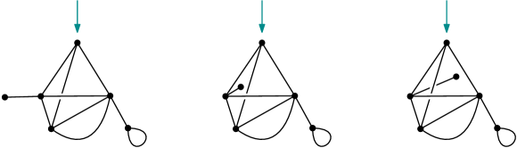
Figure 1. Three rooted maps. Each root is marked by an arrow. The two last maps are equal.

Definition 2 (Map features).

A face can be obtained by starting at some corner, moving along an incident half-edge, then switching to the next clockwise half-edge and repeating the procedure until the starting corner is met. A loop is an edge that connects the same vertex. An isthmus is an edge such that the deletion of this edge increases the number of connected components of the underlying graph. The degree of a vertex is the number of half-edges incident to this vertex.

These definitions are illustrated in Figure 2 (right).

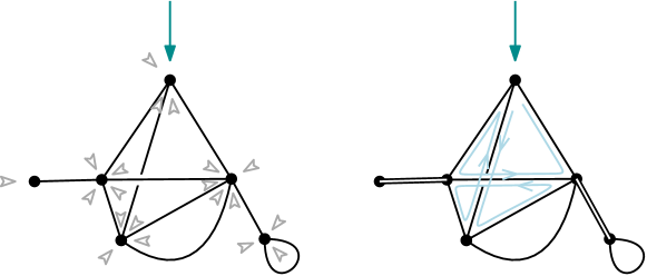
Figure 2. Left: The small triangles point at every corner of the map. Right: The light-blue line marks the contour of one face of the map. The double-lined edges are the isthmi of the map. The only loop of the map is adjacent to the rightmost isthmus, and the vertex incident to this loop has degree $3$.

Arquès and Béraud [AB00] prove that the generating function of maps $M(z):=\sum_{n\geqslant 0}m_{n}z^{n}$, where $m_{n}$ enumerates the number of maps with $n$ edges, satisfies

(1) $$2z^{2}M^{\prime}(z)=(1-z)M(z)-1-zM(z)^{2},$$

a typical Riccati equation whose first few Taylor coefficients read $M(z)=1+2z+20z^{2}+444z^{3}+16944z^{4}+\cdots$.

Table 1. The six map statistics and their limit laws studied in this extended abstract.

Statistics	Differential equation	Mean	Limit law
leaves	$\hbox to0.0pt{$\;L$\hss}{\hphantom{M}}=v+(2-u)zL+zL^{2}$	$1$	$\operatorname{Poisson}(1)$
	$\qquad{}+2z^{2}\partial_{z}L+z(1-v)\partial_{v}L$
root isthmic parts	$\hbox to0.0pt{$\;C$\hss}{\hphantom{M}}=1+zC+vzC|_{v=1}C+2z^{2}\partial_{z}C$	$2$	$\operatorname{Geometric}(\frac{1}{2})$
vertices	$\hbox to0.0pt{$\;X$\hss}{\hphantom{M}}=v+zX+zX^{2}+2z^{2}\partial_{z}X$	$\log n$	$\mathcal{N}(\log n,\log n)$
loops	$\hbox to0.0pt{$\;Y$\hss}{\hphantom{M}}=v+vzY+vzY|_{v=1}Y$	$\frac{1}{2}n$	$\text{A new law}^{*}$
	$\qquad{}+2vz^{2}\partial_{z}Y+v^{2}z(vw-1)\partial_{v}Y$
root edges	$\hbox to0.0pt{$\;E$\hss}{\hphantom{M}}=1+vzE+vzE|_{v=1}E$	$\frac{2}{3}n$	$\operatorname{Beta}(1,\frac{1}{2})$
	$\qquad{}+2vz^{2}\partial_{z}E$
root degree	$\hbox to0.0pt{$\;D$\hss}{\hphantom{M}}=1+v^{2}zD+vzD|_{v=1}D$	$n$	$\text{Uniform}[0,2]$
	$\qquad{}+2vz^{2}\partial_{z}D-v^{2}(1-v)z\partial_{v}D$

1.3. Results and methods

We address in this paper the analysis of the extended equations of (1) for bivariate (and in one case, trivariate) generating functions $M(z,v):=\sum_{n,k\geqslant 0}m_{n,k}z^{n}v^{k}$, where $m_{n,k}$ stands for the number of maps with $n$ edges and the value of the shape parameter equal to $k$. We obtain limit laws for the distributions of six different parameters (see Figures 3, 3, 4, 4, 5 and 5).

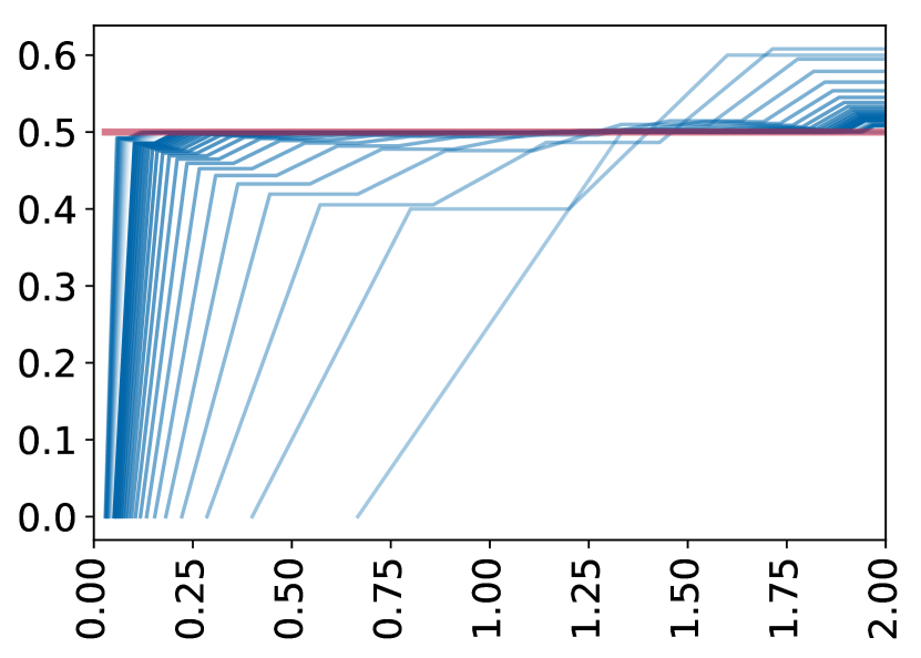
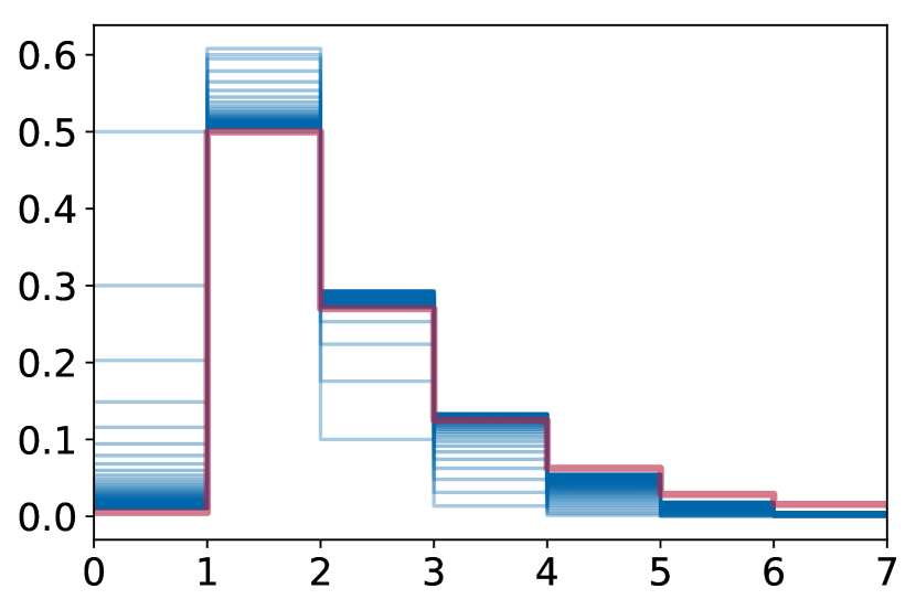
Figure 3. Left: Root vertex degree. Right: Number of root isthmic parts.

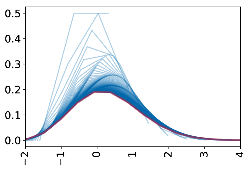
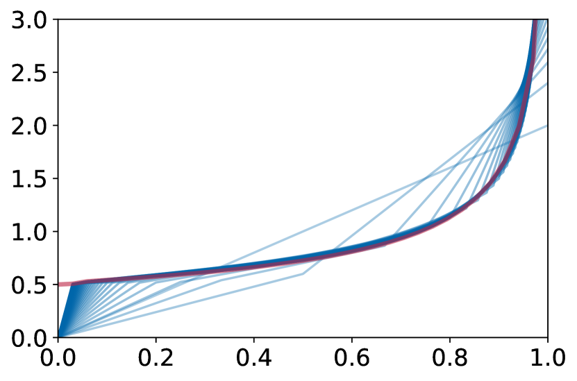
Figure 4. Left: Number of vertices. Right: Number of root edges.

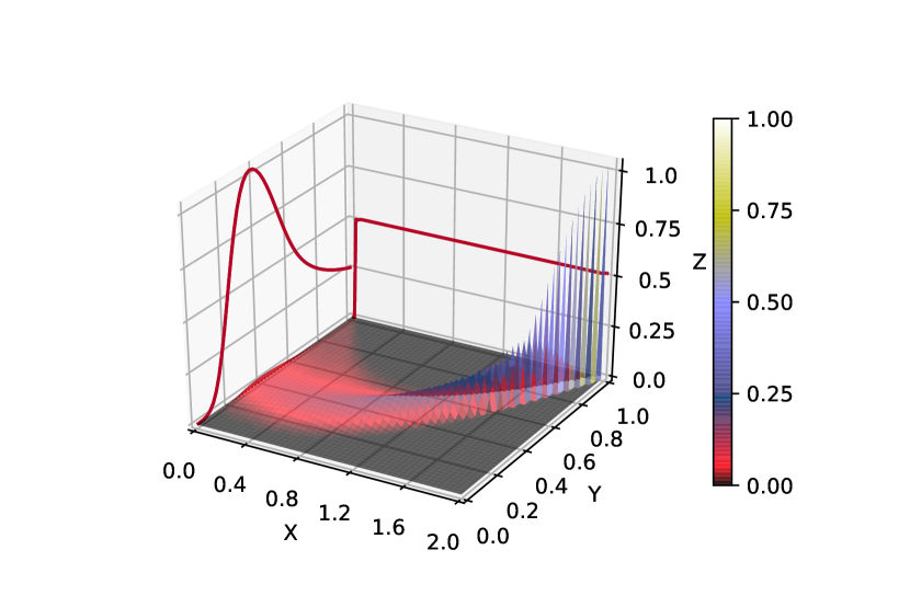
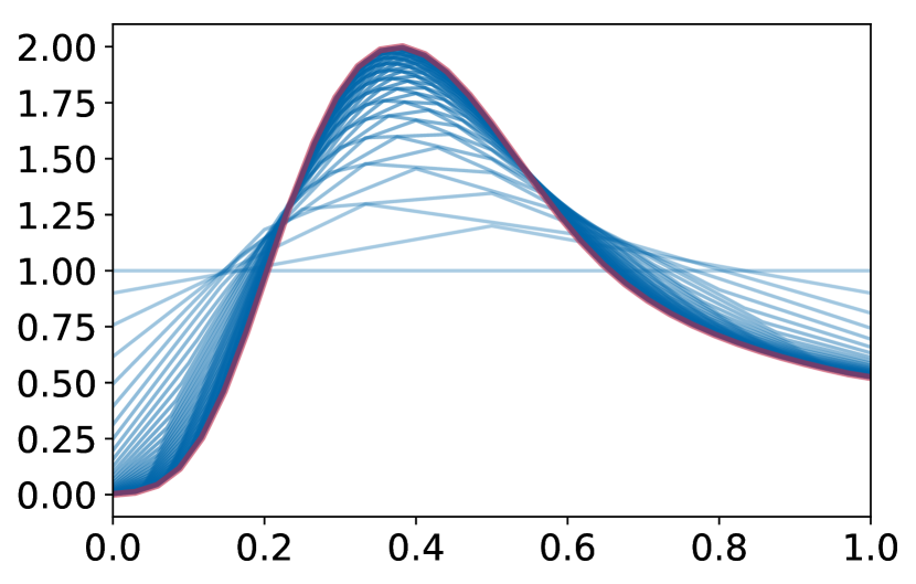
Figure 5. Left: Joint distribution of root vertex degree and the number of loops. Right: Number of loops.

We collect the statistics and their limit laws studied here in Table 1 for comparison. We see that some of the limit laws are discrete (Poisson and Geometric), one of them (the number of vertices) is Gaussian with a logarithmic mean, which we denote by $\mathcal{N}(\log n,\log n)$, and the others are continuous. For the number of root edges, root degree and loops, the corresponding limit laws are normalized by $n$, the total number of edges. The distribution of the number of loops follows a rather unusual limit law (see Figure 5) in the sense that we can only characterise the limit law by its moment sequence, $\eta_{l}$, which satisfies $\eta_{l}=\eta_{0,l}$ with $\eta_{k,l}$ computable only through a recurrence involving $\eta_{k-1,l}$ and $\eta_{k+1,l-1}$. The corresponding probability density function of this law remains unknown and does not have an explicit expression at this stage (see Figure 5). Finally, by the bijection from [CYZ16] and a known property of chord diagrams in [FN00], it is possible to deduce the limit laws for the number of leaves.

One technique we use several times in our proofs consists in linearising the differential equations satisfied by the generating functions, by choosing a suitable transformation, inspired from the resolution of Riccati equations. Once the dominant term is identified, the analysis for the limit law becomes more or less straightforward. When such a technique fails, we rely then on the method of moments, which establishes weak convergence by computing all higher derivatives of $M(z,v)$ at $v=1$ and by examining asymptotically the ratios $[z^{n}]\partial_{v}^{k}M(z,v)|_{v=1}/[z^{n}]M(z,1)$ (which correspond to the moments of random variable). Such a procedure also linearises to some extent the more complicated bivariate nature of the differential equations and facilitates the resolution complexity of the asymptotic problem.

Structure of the Paper.

In Section 2 we derive the nonlinear differential equations satisfied by the generating functions of the map statistics. Then in Section 3 we sketch the proofs for the limit laws of five statistics based on generating functions. The Poisson law for the number of leaves (together with the root face degree and the number of trivial loops) will be proved by a direct combinatorial approach in the last section.

2. Differential equations for maps

In this section, we derive the differential equations satisfied by the bivariate or trivariate generating functions with the additional variable(s) counting the shape statistics.

Univariate generating function of maps.

Since the Riccati equation (1) lies at the basis of all other extended equations in Table 1, we give a quick proof of it via the recurrence satisfied by $m_{n}$, the number of maps with $n$ edges (see Figure 6):

(2) $$m_{n}=\boldsymbol{1}_{[n=0]}+\sum_{0\leqslant k<n}m_{k}m_{n-1-k}+(2n-1)m_{n-1},$$

which then implies the Riccati equation (1).

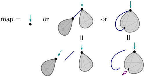
Figure 6. A symbolic construction of rooted maps.

First, $m_{0}=1$ because there is only one map with $0$ edges. Then a map with $n$ edges can be formed either by connecting the roots of two maps (with $k$ and $n-k-1$ edges, respectively) with an isthmus, or by adding an edge to a map with $n-1$ edges, connecting the root and a corner. The number of possible ways to insert an edge in this way is equal to $2n-1$, because there are $2n-2$ corners in a map of size $n-1$, and there are two possible ways to insert a new edge at the root corner (either before, or after the root). This proves (2).

Vertices.

Consider now the bivariate generating function $X(z,v)=\sum_{n,k\geqslant 0}x_{n,k}z^{n}v^{k},$ where $x_{n,k}$ is equal to the number of rooted maps with $n$ edges and $k$ vertices. Arquès and Béraud [AB00] showed that

(3) $$X(z,v)=v+zX(z,v)+zX(z,v)^{2}+2z^{2}\partial_{z}X(z,v).$$

This recurrence can be obtained from (2) by noticing that no new vertex is created when we connect two maps with an isthmus, nor when we add a new root edge to a map. Note that $X(z,v)$ satisfies another functional equation (see [AB00])

$$X(z,v)=v+zX(z,v)X(z,v+1),$$

which seems less useful from an asymptotic point of view.

Root isthmic parts.

We count here the root isthmic parts, which are the number of isthmic constructions used at the root vertex. Note that an isthmic part may not be a bridge because the additional edge constructor may induce additional connections.

We show that the bivariate generating function $C(z,v)=\sum_{n,k\geqslant 0}c_{n,k}z^{n}v^{k}$, where $c_{n,k}$ enumerates the number of maps with $n$ edges and $k$ root isthmic parts, satisfies

(4) $$C(z,v)=1+zC(z,v)+vzC(z,v)C(z,1)+2z^{2}\partial_{z}C(z,v).$$

In Figure 6, the number of root isthmic parts only changes whenever two maps are connected by an isthmus. This yields $vzC(z,v)C(z,1)$ instead of $zC^{2}$.

Root edges.

Similarly, consider $E(z,v)=\sum_{n,k\geqslant 0}e_{n,k}z^{n}v^{k}$, where $e_{n,k}$ counts the number of rooted maps with $n$ edges and $k$ root edges. We show that $E(z,v)$ satisfies

(5) $$E=1+vzE+vzE|_{v=1}E+2vz^{2}\partial_{z}E.$$

This again results from the recurrence (2) and from Figure 6: the non-root edges come from the bottom map in the isthmic construction, yielding the term $vzE(z,v)E(z,1)$.

Root Degree.

Consider the degree of the root vertex. Note that this may be different from the number of root edges because for the root degree, each loop edge is counted twice, therefore the degree of the root vertex varies from $0$ to $2n$. By duality, the distribution of the root face degree is the same as the distribution of the root vertex degree.

Let $D(z,v)=\sum_{n,k\geqslant 0}d_{n,k}z^{n}v^{k}$ denote the bivariate generating function for maps with variable $v$ marking root degree. Then

(6) $$D=1+v^{2}zD+vzD|_{v=1}D+2vz^{2}\partial_{z}D-v^{2}(1-v)z\partial_{v}D.$$

In this case, the original construction in Figure 6 is insufficient, and we need to consider further cases in Figure 7. When an additional edge becomes a loop, it increases the degree of the root vertex by $2$; otherwise, the root degree is increased merely by $1$. Note that the equation (6) is now a bona fide partial differential equation, making the analysis more difficult.

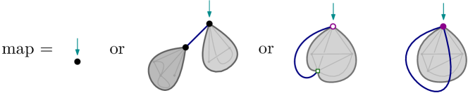
Figure 7. Symbolic method to count root degree and loops in rooted maps.

Leaves.

The differential equation for the bivariate generating function of maps with variable $v$ marking leaves (see Table 1) can be obtained in a similar way by considering different cases in the new edge constructor. The number of special leaf corners is equal to the number of leaves.

Loops.

Finally, we look at the number of loops whose enumeration necessitates the consideration of the joint distribution of the number of loops and the number of root edges, namely, we consider the trivariate generating function $Y(z,v,w)=\sum_{n,k,m}y_{n,k,m}z^{n}v^{k}w^{m}$, where $y_{n,k,m}$ denotes the number of rooted maps with $n$ edges, root degree equal to $k$, and $m$ loops. We show that $Y(z,v,w)$ satisfies a partial differential equation

(7) $$Y=1+zvY+zvY|_{v=1}Y+2z^{2}v\partial_{z}Y+zv^{2}(vw-1)\partial_{v}Y.$$

As in the symbolic construction of Figure 7, a new edge becomes a loop only if it is attached to one of the corners incident to the root vertex. The differential equation (7) is then a modification of (6) with an additional variable counting the number of loops.

Note that Equation (7) is catalytic with respect to the variable $v$, i.e. putting $v=1$ introduces a new unknown object $\partial_{v}Y|_{v=1}$ to the differential equation. One of the strategies for dealing with catalytic equations was developed by Bousquet-Mélou and Jehanne [BMJ06], generalising the so-called kernel method and quadratic method. However, their method does not work in our case because our equation is differentially algebraic.

3. Limit laws

This section describes the techniques we employ to establish the limit laws.

From now on, by a random map (with $n$ edges) we assume that all rooted map with $n$ edges are equally likely. For notational convention, we use $X^{\prime}=\partial_{z}X$ to denote derivative with respect to $z$. Due to space limit, we give only the sketches of the proofs.

3.1. Transformation into a linear differential equation

For most of the equations in the previous section, it turns out that a transformation similar to that used for Riccati equations largely simplifies the resolution and leads to solvable recurrences, which are then suitable for our asymptotic purposes. We begin by solving the standard Riccati equation (1) and see how a similar idea extends to other differential equations.

Proposition 3.

The number $m_{n}$ of maps with $n$ edges satisfies

(8) $$\frac{m_{n}}{\phi_{n}}=2n-1+O\bigl{(}n^{-1}\bigr{)},\quad\textrm{where}\quad\phi_{n}=\dfrac{(2n)!}{2^{n}n!}=(2n-1)!!.$$

Proof.

We solve the Riccati equation (1) by considering the transformation

(9) $$M(z)=1+\dfrac{2z\phi^{\prime}(z)}{\phi(z)},$$

for some function $\phi(z)$ with $\phi(0)=1$. Substituting this form into the equation (2), we get the second-order differential equation $2z^{2}\phi^{\prime\prime}+(5z-1)\phi^{\prime}+\phi=0$. From this equation, the coefficients $\phi_{n}:=[z^{n}]\phi(z)$ satisfy the recurrence $\phi_{n+1}=(2n+1)\phi_{n}$, which implies the double factorial form of $\phi_{n}$ by $\phi_{0}=1$.

Moreover, by extracting the coefficient of $z^{n}$ in (9), we obtain a relation between the coefficients $m_{k}$ and $\phi_{\ell}$. By the inequality $m_{n}\geqslant(2n-1)m_{n-1}$ (see (2)), we then deduce the asymptotic relation (8). ∎

Theorem 4.

Let $X_{n}$ denote the number of vertices in a random rooted map with $n$ edges. Then $X_{n}$ follows a central limit theorem with logarithmic mean and logarithmic variance:

(10) $$\dfrac{X_{n}-\mathbb{E}(X_{n})}{\sqrt{\operatorname{\mathbb{V}}(X_{n})}}\overset{d}{\longrightarrow}\mathcal{N}(0,1),\quad\mathbb{E}(X_{n})\sim\log n,\quad\operatorname{\mathbb{V}}(X_{n})\sim\log n.$$

Proof.

Similar to (9), we define a bivariate generating function $S(z,v)=\sum_{n\geqslant 0}s_{n}(v)z^{n}$ such that

$$X(z,v)=v+\dfrac{2zS^{\prime}}{S},\quad S(0)=1.$$

Substituting this $X(z,v)$ into (3) leads to a linear differential equation from which one can extract the recurrence

$$s_{n}(v)=\dfrac{(2n+v-2)(2n+v-1)}{2n}\,s_{n-1}(v).$$

We then get an explicit expression for $s_{n}(v)$, from which we deduce, by singularity analysis, that

$$\mathbb{E}(v^{X_{n}})=\dfrac{2^{v-1}}{\Gamma(v)}\,n^{v-1}(1+O(n^{-1})),$$

and conclude by applying the Quasi-Powers Theorem [FS09, Hwa98]. ∎

A finer Poisson$(\log n+c)$ approximation, for a suitably chosen $c$, is also possible, which results in a better convergence rate $O(\log n)^{-1}$ instead of $(\log n)^{-\frac{1}{2}}$; see [Hwa99] for details.

Theorem 5.

Let $C_{n}$ denote the number of root isthmic parts in a random rooted map with $n$ edges. Then,

$$C_{n}\overset{d}{\longrightarrow}\operatorname{Geometric}\bigl{(}\tfrac{1}{2}\bigr{)}.$$

Proof.

Since $C(1,z)=M(z)$, we use again the substitution (9) and apply it to (4):

$$2z^{2}(\phi C^{\prime}+v\phi^{\prime}C)=(1-(1+v)z)\phi C-\phi.$$

The trick here is to multiply both sides by $\phi(z)^{v-1}$ and set $Q(z,v)=\phi(z)^{v}C(z,v)$. We then obtain

$$2z^{2}Q^{\prime}=(1-(1+v)z)Q-\phi^{v}.$$

Using the recurrence for the normalised coefficients $\widehat{q}_{n}(v):=q_{n}(v)/\phi_{n}$ and dominant-term approximations, we find that the $n$-th coefficient of $Q$ is proportional to

$$\widehat{q}_{n}(v)=\dfrac{v}{2n}\sum_{1\leqslant k\leqslant n}\left(\dfrac{n}{k}\right)^{v/2}+O(n^{-1/2})=\dfrac{v}{2-v}+O(n^{-\frac{1}{2}}).$$

This corresponds to a (shifted by $1$) geometric distribution with parameter $\frac{1}{2}$. By the definition $Q(z,v)=\phi(z)^{v}C(z,v)$, we deduce that the limiting distribution of $C_{n}$ is also geometric with parameter $\frac{1}{2}$. ∎

Theorem 6.

Let $E_{n}$ denote the number of edges incident to the root vertex in a random rooted map with $n$ edges. Then $E_{n}$ follows asymptotically a Beta distribution:

(11) $$\dfrac{E_{n}}{n}\overset{d}{\longrightarrow}\operatorname{Beta}\bigl{(}1,\tfrac{1}{2}\bigr{)},$$

with the density function $\frac{1}{2}(1-t)^{-\frac{1}{2}}$ for $t\in[0,1)$.

Proof.

We use again the substitution $E(z,1)=M(z)=1+2z\frac{\phi^{\prime}}{\phi}$ in (5), giving

$$2vz^{2}(\phi E^{\prime}+\phi^{\prime}E)=(1-2vz)\phi E-\phi.$$

With $Q(z,v)=\phi(z)E(z,v)$, we then obtain

(12) $$2vz^{2}Q^{\prime}=(1-2vz)Q-\phi.$$

This linear differential equation translates into a recurrence for the coefficients $q_{n}(v)$ of $Q(z,v)$, which yields the closed-form expression

(13) $$q_{n}(v)=2^{n}n!\sum_{0\leqslant j\leqslant n}{2j\choose j}4^{-j}v^{n-j}.$$

Returning to $E(z,v)$, we see that its coefficients behave asymptotically like $q_{n}(v)$. This implies the Beta limit law (11) for the random variable $E_{n}/n$ since $\binom{2j}{j}4^{-j}\sim(\pi j)^{-1/2}$ for large $j$. ∎

Theorem 7.

Let $D_{n}$ denote the degree of the root vertex in a random rooted map with $n$ edges. Then, $D_{n}$, divided by the number of edges, converges in law to the uniform distribution on $[0,2]$:

(14) $$\dfrac{D_{n}}{n}\overset{d}{\longrightarrow}\operatorname{Uniform}\left[0,2\right].$$

Proof.

The substitutions

$$D(z,1)=M(z)=1+\dfrac{2z\phi^{\prime}}{\phi},\quad\text{and}\quad D(z,v)=\dfrac{Q(z,v)}{\phi(z)}$$

lead to a partial differential equation, which in turn yields the recurrence for the coefficients $q_{n}(v):=[z^{n}]Q(z,v)$:

$$q_{n}(v)=v(2n-1+v)q_{n-1}-v^{2}(1-v)q_{n-1}^{\prime}(v)+\phi_{n}.$$

We then get the exact solution $q_{n}(v)=\phi_{n}(1+v+\cdots+v^{2n})$. Accordingly, $d_{n}(v):=[z^{n}]D(z,v)\sim q_{n}(v)$. This implies the uniform limit law (14). ∎

A more intuitive interpretation of this uniform limit law is given in the next section.

3.2. Approximation and method of moments

Unlike all previous proofs, we use the method of moments to establish the limiting distribution of the number of loops. The situation is complicated by the presence of the term involving $\partial_{v}Y$ in (7), which introduces higher order derivatives with respect to $v$ at $v=1$ when computing the asymptotic of the moments.

Theorem 8.

Let $Y_{n}$ denote the total number of loops in a random rooted map with $n$ edges. Then

(15) $$\dfrac{Y_{n}}{n}\overset{d}{\longrightarrow}\mathcal{L},$$

where $\mathcal{L}$ is a continuous law with a computable density on $[0,1]$.

Proof.

First, we show by induction that there exist constants $\eta_{k,\ell}$, such that as $n\to\infty$,

(16) $$\left.[z^{n}]\partial_{v}^{k}\partial_{w}^{\ell}Y(z,v,w)\right|_{v=w=1}\sim\eta_{k,\ell}n^{k+\ell+1}\phi_{n},\quad k,\ell\geqslant 0.$$

For $k=\ell=0$ the statement clearly holds. Let $y_{n}^{(k,\ell)}:=\left.[z^{n}]\partial_{v}^{k}\partial_{w}^{\ell}Y(z,v,w)\right|_{v=w=1}$ for larger $k,\ell\geqslant 0$. By translating (7) into the corresponding recurrence for the coefficients and by collecting the dominant terms (using the induction hypothesis (16)), we deduce that

$$y_{n}^{(k,\ell)}\sim(2n+k)y_{n-1}^{(k,\ell)}+\ell y_{n-1}^{(k+1,\ell-1)}+(2kn-2k)y_{n-1}^{(k-1,\ell)}+\boldsymbol{1}_{[k=0]}y_{n-1}^{(k,\ell)}.$$

Accordingly, we are led to the recurrence

$$\eta_{k,\ell}=\dfrac{1}{k+2\ell+\boldsymbol{1}_{[k>0]}}(2k\eta_{k-1,\ell}+\ell\eta_{k+1,\ell-1}),$$

for $k+\ell>0$ (provided that we interpret $\eta_{k,\ell}=0$ when any index becomes negative). In particular, when $\ell=0$, we obtain the moments of the random variable $E_{n}$, the number of root edges: $\eta_{k,0}=\frac{2^{k+1}}{k+1}$, which coincides with the moments of the uniform random variable $\operatorname{Uniform}[0,2]$. Finally, it is not complicated to check that the numbers $\eta_{0,\ell}$ satisfy the condition of Hausdorff moment problem, i.e. $\eta_{0,\ell}$ uniquely determine the limiting random variable defined on $[0,1]$. ∎

4. Combinatorics of map statistics

We examine briefly the combinatorial aspect of the map statistics, relying our arguments on the close connection between maps and chord diagrams (see [Cor09]).

Recall that a chord diagram [FN00] with $n$ chords is a set of vertices labelled with the numbers $\{1,2,\ldots,2n\}$ equipped with a perfect matching. A chord diagram is indecomposable if it cannot be expressed as a concatenation of two smaller diagrams.

Why the root degree follows a uniform law?

We begin with Cori’s bijection [Cor09] between rooted maps and indecomposable diagrams. In this bijection, each chord connecting labels $i$ and $j$ corresponds to matching of the half-edges with labels $i$ and $j$. The set of half-edges incident to each vertex of the resulting map corresponds to the set of nodes to the right of the starting points of the so-called outer chords, i.e. chords that do not lie under any other chord.

Proposition 9.

There exists a bijection between rooted maps of root degree $d$ with $n$ edges, and indecomposable diagrams with $n+1$ chords such that the vertex $k-2$ is matched with vertex $1$.

Once this proposition is available, it leads to a simpler and more intuitive proof of Theorem 7 as follows. In a (not necessarily indecomposable) diagram, the label of the vertex matched with $1$ follows exactly a uniform law on $\{2,\dots,2n\}$. But a diagram is almost surely an indecomposable diagram (because its cardinality is asymptotically the same); thus the label of the vertex matched with $1$ divided by $2n$ obeys asymptotically a uniform law on $[0,1]$ (or Uniform$[0,2]$ if divided by $n$ as in Theorem 7).

Uniform random generation.

Cori’s bijection is also useful for generating random rooted maps. Uniformly sampling a random diagram can be achieved by adding the chords sequentially one after another. If this procedure results in an indecomposable diagram, it is rejected (which occurs with asymptotic probability $0$). A successful sampled diagram is then transformed into a map using Cori’s bijection [Cor09]. Figure 8 shows two instances of random maps thus generated.

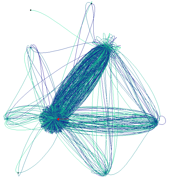
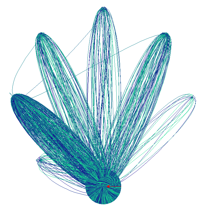
Figure 8. Random rooted maps, respectively with $1000$ and $20000$ edges.

The number of leaves.

Another bijection in [CYZ16] is useful in proving the Poisson limit law of the number of leaves. This bijection sends leaves of a map into the isolated chords (namely, edges connecting vertices $k$ and $k+1$) of an indecomposable chord diagram. According to [FN00, Theorem 2], the number of isolated edges in a random chord diagram has a Poisson distribution with parameter $1$. We can then deduce the following theorem.

Theorem 10.

The number of leaves in a random map with $n$ edges follows asymptotically a Poisson law with parameter $1$.

Two dual parameters.

We briefly remark that two other parameters, namely root face degree and the number of trivial loops do not seem easily dealt with by the method of generating functions because marking them requires additional nested information such as the degrees of all the faces. However, such parameters can be easily marked in their corresponding dual maps. Their limit distributions are uniform and Poisson, respectively.

References

- [AB00] Didier Arquès and Jean-François Béraud. Rooted maps on orientable surfaces, Riccati’s equation and continued fractions. Discrete mathematics, 215(1-3):1–12, 2000.
- [BBM17] Olivier Bernardi and Mireille Bousquet-Mélou. Counting coloured planar maps: differential equations. Communications in Mathematical Physics, 354(1):31–84, 2017.
- [BFSS01] Cyril Banderier, Philippe Flajolet, Gilles Schaeffer, and Michele Soria. Random maps, coalescing saddles, singularity analysis, and Airy phenomena. Random Structures & Algorithms, 19(3-4):194–246, 2001.
- [BGJ13] Olivier Bodini, Danielle Gardy, and Alice Jacquot. Asymptotics and random sampling for BCI and BCK lambda terms. Theoretical Computer Science, 502:227–238, 2013.
- [BMJ06] Mireille Bousquet-Mélou and Arnaud Jehanne. Polynomial equations with one catalytic variable, algebraic series and map enumeration. Journal of Combinatorial Theory, Series B, 96(5):623–672, 2006.
- [BR86] Edward A Bender and L.Bruce Richmond. A survey of the asymptotic behaviour of maps. Journal of Combinatorial Theory, Series B, 40(3):297 – 329, 1986.
- [CacLP78] Predrag Cvitanović, B. Lautrup, and Robert B. Pearson. Number and weights of Feynman diagrams. Phys. Rev. D, 18:1939–1949, Sep 1978.
- [Car17] Ariane Carrance. Uniform random colored complexes. arXiv preprint arXiv:1705.11103, 2017.
- [Cor09] Robert Cori. Indecomposable permutations, hypermaps and labeled Dyck paths. Journal of Combinatorial Theory, Series A, 116(8):1326–1343, 2009.
- [CY17] Julien Courtiel and Karen Yeats. Terminal chords in connected chord diagrams. Annales de l’Institut Henri Poincaré D, 4(4):417–452, 2017.
- [CYZ16] Julien Courtiel, Karen Yeats, and Noam Zeilberger. Connected chord diagrams and bridgeless maps. arXiv preprint arXiv:1611.04611, 2016.
- [DP13] Michael Drmota and Konstantinos Panagiotou. A central limit theorem for the number of degree-k vertices in random maps. Algorithmica, 66(4):741–761, 2013.
- [FN00] Philippe Flajolet and Marc Noy. Analytic combinatorics of chord diagrams. In Formal Power Series and Algebraic Combinatorics, pages 191–201. Springer, 2000.
- [FS09] Philippe Flajolet and Robert Sedgewick. Analytic combinatorics. Camb. Univ. Press, 2009.
- [Hwa98] Hsien-Kuei Hwang. On convergence rates in the central limit theorems for combinatorial structures. European Journal of Combinatorics, 19(3):329–343, 1998.
- [Hwa99] Hsien-Kuei Hwang. Asymptotics of poisson approximation to random discrete distributions: an analytic approach. Advances in Applied Probability, 31(2):448–491, 1999.
- [Lis99] Valery A. Liskovets. A pattern of asymptotic vertex valency distributions in planar maps. Journal of Combinatorial Theory, Series B, 75(1):116–133, 1999.
- [LZ04] Sergei K. Lando and Alexander K. Zvonkin. Graphs on Surfaces and Their Applications. Number 141 in Encyclopaedia of Mathematical Sciences. Springer-Verlag, 2004.
- [Odl95] Andrew M. Odlyzko. Asymptotic enumeration methods. Handbook of combinatorics, 2(1063-1229):1229, 1995.
- [Slo] N. J. A. Sloane. The On-Line Encyclopedia of Integer Sequences.
- [ZG15] Noam Zeilberger and Alain Giorgetti. A correspondence between rooted planar maps and normal planar lambda terms. Logical Methods in Computer Science, 11(3:22), 2015.