Temporal Vertex Cover with a Sliding Time Window

Abstract

Modern, inherently dynamic systems are usually characterized by a network structure, i.e. an underlying graph topology, which is subject to discrete changes over time. Given a static underlying graph $G$, a temporal graph can be represented via an assignment of a set of integer time-labels to every edge of $G$, indicating the discrete time steps when this edge is active. While most of the recent theoretical research on temporal graphs has focused on the notion of a temporal path and other “path-related” temporal notions, only few attempts have been made to investigate “non-path” temporal graph problems. In this paper, motivated by applications in sensor and in transportation networks, we introduce and study two natural temporal extensions of the classical problem Vertex Cover. In both cases we wish to minimize the total number of “vertex appearances” that are needed to “cover” the whole temporal graph. In our first problem, Temporal Vertex Cover, the aim is to cover every edge at least once during the lifetime of the temporal graph, where an edge can be covered by one of its endpoints, only at a time step when it is active. In our second, more pragmatic variation Sliding Window Temporal Vertex Cover, we are also given a natural number $\Delta$, and our aim is to cover every edge at least once at every $\Delta$ consecutive time steps. We present a thorough investigation of the computational complexity and approximability of these two temporal covering problems. In particular, we provide strong hardness results, complemented by various approximation and exact algorithms. Some of our algorithms are polynomial-time, while others are asymptotically almost optimal under the Exponential Time Hypothesis (ETH) and other plausible complexity assumptions.

Keywords: Temporal networks, temporal vertex cover, Exponential Time Hypothesis (ETH), approximation algorithm, approximation hardness.

1 Introduction and Motivation

A great variety of both modern and traditional networks are inherently dynamic, in the sense that their link availability varies over time. Information and communication networks, social networks, transportation networks, and several physical systems are only a few examples of networks that change over time [27, 40]. The common characteristic in all these application areas is that the network structure, i.e. the underlying graph topology, is subject to discrete changes over time. In this paper we adopt a simple and natural model for time-varying networks which is given with time-labels on the edges of a graph, while the vertex set remains unchanged. This formalism originates in the foundational work of Kempe et al. [30].

Definition 1 (temporal graph).

A temporal graph is a pair $(G,\lambda)$, where $G=(V,E)$ is an underlying (static) graph and $\lambda:E\rightarrow 2^{\mathbb{N}}$ is a time-labeling function which assigns to every edge of $G$ a set of discrete-time labels.

For every edge $e\in E$ in the underlying graph $G$ of a temporal graph $(G,\lambda)$, $\lambda(e)$ denotes the set of time slots at which $e$ is active in $(G,\lambda)$. Due to its vast applicability in many areas, this notion of temporal graphs has been studied from different perspectives under various names such as time-varying [22, 44, 1], evolving [9, 21, 15], dynamic [24, 12], and graphs over time [34]; for a recent attempt to integrate existing models, concepts, and results from the distributed computing perspective see the survey papers [12, 10, 11] and the references therein. Data analytics on temporal networks have also been very recently studied in the context of summarizing networks that represent sports teams’ activity data to discover recurring strategies and understand team tactics [32], as well as extracting patterns from interactions between groups of entities in a social network [31].

Motivated by the fact that information in temporal graphs can “flow” only along sequences of edges whose time-labels are increasing, most temporal graph parameters and optimization problems that have been studied so far are based on the notion of temporal paths and other “path-related” notions, such as temporal analogues of distance, diameter, reachability, exploration, and centrality [2, 19, 36, 39, 3, 18, 4, 5]. In contrast, only few attempts have been made to define “non-path” temporal graph problems. Motivated by the contact patterns among high-school students, Viard et al. [46, 47], and later Himmel et al. [26], introduced and studied $\Delta$-cliques, an extension of the concept of cliques to temporal graphs, in which all vertices interact with each other at least once every $\Delta$ consecutive time steps within a given time interval. Furthermore, natural temporal extensions have been recently introduced and studied for the classical problems graph coloring [38] and maximum matching [8, 37].

In this paper we introduce and study two natural temporal extensions of the problem Vertex Cover in static graphs, which take into account the dynamic nature of the network. In the first and simpler of these extensions, namely Temporal Vertex Cover (for short, TVC), every edge $e$ has to be “covered” at least once during the lifetime $T$ of the network (by one of its endpoints), and this must happen at a time step $t$ when $e$ is active. The goal is then to cover all edges with the minimum total number of such “vertex appearances”. On the other hand, in many real-world applications where scalability is important, the lifetime $T$ can be arbitrarily large but the network still needs to remain sufficiently covered. In such cases, as well as in safety-critical systems (e.g. in military applications), it may not be satisfactory enough that an edge is covered just once during the whole lifetime of the network. Instead, every edge must be covered at least once within every small $\Delta$-window of time in which it is active (for an appropriate value of $\Delta$), regardless of how large the lifetime is; this gives rise to our second optimization problem, namely Sliding Window Temporal Vertex Cover (for short, SW-TVC). Formal definitions of our problems TVC and SW-TVC are given in Section 2. Here it is worth mentioning that very recently another temporal version of Vertex Cover –namely the network-untangling problem– has been introduced and studied, motivated by applications in discovering events’ timelines from complex interactions among entities [43].

Our main motivation for introducing and studying TVC and SW-TVC is of theoretical nature, namely to lift one of the most classical optimization problems, such as Vertex Cover, to the temporal setting. However, these temporal extensions of Vertex Cover could potentially also prove useful in extending the known practical applications of the static Vertex Cover problem. One example of such a possible application comes from the field of sensor networks, where several works considered problems of placing sensors to cover a whole area or multiple critical locations, e.g. for reasons of surveillance. Such studies usually wish to minimize the number of sensors used or the total energy required [33, 25, 17, 48, 42].

1.1 Our contribution

In this paper we present a thorough investigation of the complexity and approximability of the problems Temporal Vertex Cover (TVC) and Sliding Window Temporal Vertex Cover (SW-TVC) on temporal graphs. We first prove in Section 3 that TVC remains NP-complete even on the special case of star temporal graphs, i.e. when the underlying graph $G$ is a star. This NP-completeness is proved via a reduction from Set Cover, which provides a natural one-to-one correspondence between the input Set Cover instance and the produced instance of TVC on star temporal graphs. Furthermore we prove that, for any $\varepsilon<1$, TVC on star temporal graphs cannot be optimally solved in $O(2^{\varepsilon T})$ time, assuming the Strong Exponential Time Hypothesis (SETH), as well as that it does not admit a polynomial-time $(1-\varepsilon)\ln{n}$-approximation algorithm, unless NP has $n^{O(\log\log n)}$-time deterministic algorithms. On the positive side we prove that, on general temporal graphs with $n$ vertices, TVC can be $(H_{n-1}-\frac{1}{2})$-approximated in polynomial time, where $H_{n}=\sum_{i=1}^{n}\frac{1}{i}\approx\ln n$ is the $n$th harmonic number.

In Section 4 and in the reminder of the paper we deal with SW-TVC. We prove in Section 4.1 a strong complexity lower bound on arbitrary temporal graphs. More specifically we prove that, for any (arbitrarily growing) functions $f:\mathbb{N}\rightarrow\mathbb{N}$ and $g:\mathbb{N}\rightarrow\mathbb{N}$, there exists a constant $\varepsilon\in(0,1)$ such that SW-TVC cannot be solved in $f(T)\cdot 2^{\varepsilon n\cdot g(\Delta)}$ time, assuming the Exponential Time Hypothesis (ETH). This ETH-based lower bound turns out to be asymptotically almost tight, as we present an exact dynamic programming algorithm with running time $O(T\Delta(n+m)\cdot 2^{n(\Delta+1)})$. This worst-case running time can be significantly improved in certain special temporal graph classes. In particular, when the “snapshot” of $(G,\lambda)$ at every time step has vertex cover number bounded by $k$, the running time becomes $O(T\Delta(n+m)\cdot n^{k(\Delta+1)})$. That is, whenever $\Delta$ is constant, this algorithm is polynomial in the input size on temporal graphs with bounded vertex cover number at every time step. Notably, when every snapshot is a star (i.e. a superclass of the star temporal graphs studied in Section 3) the running time of the algorithm is $O(T\Delta(n+m)\cdot 2^{\Delta})$.

In Section 5 we prove strong inapproximability results for SW-TVC, even in the special case where the length of the sliding window is $\Delta=2$. In particular, we prove that, unless P=NP, this problem does not admit a Polynomial Time Approximation Scheme (PTAS) even when $\Delta=2$, the maximum degree in the underlying graph $G$ is at most $3$, and every connected component of every snapshot has at most $7$ vertices. Finally, in Section 6 we provide a series of approximation algorithms for the general SW-TVC problem, with respect to various incomparable temporal graph parameters. In particular, we provide polynomial-time approximation algorithms with approximation ratios (i) $\ln{n}+\ln{\Delta}+\frac{1}{2}$, (ii) $2k$, where $k$ is the maximum number of times that each edge can appear in a sliding $\Delta$ time window (thus implying a ratio of $2\Delta$ in the general case), (iii) $d$, where $d$ is the maximum vertex degree at every snapshot of $(G,\lambda)$. Note that, for $d=1$, the latter result implies that SW-TVC can be optimally solved in polynomial time whenever every snapshot of $(G,\lambda)$ is a matching.

2 Preliminaries and notation

A theorem proving that a problem is NP-hard does not provide much information about how efficiently (although not polynomially, unless P=NP) this problem can be solved. In order to prove some useful complexity lower bounds, we mostly need to rely on some complexity hypothesis that is stronger than“P $\neq$ NP”. Impagliazzo, Paturi, and Zane formulated the Exponential Time Hypothesis (ETH) [29], which is one of the established and most well-known complexity hypotheses.

Exponential Time Hypothesis (ETH [29]).

There exists an $\varepsilon<1$ such that 3SAT cannot be solved in $O(2^{\varepsilon n})$ time, where $n$ is the number of variables in the input 3-CNF formula.

In addition to formulating ETH, Impagliazzo and Paturi proved the celebrated Sparsification Lemma [28], which has the following theorem as a consequence. This result is quite useful for providing lower bounds assuming ETH, as it expresses the running time in terms of the size of the input 3-CNF formula, rather than only the number of its variables.

Theorem 1 ([28]).

3SAT can be solved in time $2^{o(n)}$ if and only if it can be solved in time $2^{o(m)}$ on 3-CNF formulas with $n$ variables and $m$ clauses.

Given a (static) graph $G$, we denote by $V(G)$ and $E(G)$ the sets of its vertices and edges, respectively. An edge between two vertices $u$ and $v$ of $G$ is denoted by $uv$, and in this case $u$ and $v$ are said to be adjacent in $G$. We consider here temporal graphs with a finite set of integer labels assigned to every edge; the maximum label assigned by $\lambda$ to an edge of $G$, called the lifetime of $(G,\lambda)$, is denoted by $T(G,\lambda)$, or simply by $T$ when no confusion arises. That is, $T(G,\lambda)=\max\{t\in\lambda(e):e\in E\}$ and $T$ is finite. For every $i,j\in\mathbb{N}$, where $i\leq j$, we denote $[i,j]=\{i,i+1,\ldots,j\}$. Throughout the paper we refer to each integer $t\in[1,T]$ as a time point (or time slot) of $(G,\lambda)$. The instance (or snapshot) of $(G,\lambda)$ at time $t$ is the static graph $G_{t}=(V,E_{t})$, where $E_{t}=\{e\in E:t\in\lambda(e)\}$. For every $i,j\in[1,T]$, where $i\leq j$, we denote by $(G,\lambda)|_{[i,j]}$ the restriction of $(G,\lambda)$ to the time slots $i,i+1,\ldots,j$, i.e. $(G,\lambda)|_{[i,j]}$ is the sequence of the instances $G_{i},G_{i+1},\ldots,G_{j}$. We assume in the remainder of the paper that every edge of $G$ appears in at least one time slot in $\{1,...,T\}$, namely $\bigcup_{t=1}^{T}E_{t}=E$.

Although some optimization problems on temporal graphs may be hard to solve in the worst case, an optimal solution may be efficiently computable when the input temporal graph $(G,\lambda)$ has special properties, i.e. if $(G,\lambda)$ belongs to a special temporal graph class (or time-varying graph class [10, 12]). To specify a temporal graph class we can restrict (a) the underlying topology $G$, or (b) the time-labeling $\lambda$, i.e. the temporal pattern in which the time-labels appear, or both.

Definition 2.

Let $(G,\lambda)$ be a temporal graph and let $\mathcal{X}$ be a class of (static) graphs. If $G\in\mathcal{X}$ then $(G,\lambda)$ is an $\mathcal{X}$ temporal graph. On the other hand, if $G_{i}\in\mathcal{X}$ for every $i\in[1,T]$, then $(G,\lambda)$ is an always $\mathcal{X}$ temporal graph.

In the remainder of the paper we denote by $n=|V|$ and $m=|E|$ the number of vertices and edges of the underlying graph $G$, respectively, unless otherwise stated. Furthermore, unless otherwise stated, we assume that the labeling $\lambda$ is arbitrary, i.e. $(G,\lambda)$ is given with an explicit list of labels for every edge. That is, the size of the input temporal graph $(G,\lambda)$ is $O\left(|V|+\sum_{t=1}^{T}|E_{t}|\right)=O(n+mT)$. In other cases, where $\lambda$ is more restricted, e.g. if $\lambda$ is periodic or follows another specific temporal pattern, there may exist a more succinct representations of the input temporal graph.

For every $u\in V$ and every time slot $t$, we denote the appearance of vertex $u$ at time $t$ by the pair $(u,t)$. That is, every vertex $u$ has $T$ different appearances (one for each time slot) during the lifetime of $(G,\lambda)$. Similarly, for every vertex subset $S\subseteq V$ and every time slot $t$ we denote the appearance of set $S$ at time $t$ by $(S,t)$. With a slight abuse of notation, we write $(S,t)=\bigcup_{v\in S}(v,t)$. A temporal vertex subset of $(G,\lambda)$ is a set $\mathcal{S}\subseteq\{(v,t):v\in V,1\leq t\leq T\}$ of vertex appearances in $(G,\lambda)$. Given a temporal vertex subset $\mathcal{S}$, for every time slot $t\in[1,T]$ we denote by $\mathcal{S}_{t}=\{(v,t):(v,t)\in\mathcal{S}\}$ the set of all vertex appearances in $\mathcal{S}$ at the time slot $t$. Similarly, for any pair of time slots $i,j\in[1,T]$, where $i\leq j$, $\mathcal{S}|_{[i,j]}$ is the restriction of the vertex appearances of $\mathcal{S}$ within the time slots $i,i+1,\ldots,j$. Note that the cardinality of the temporal vertex subset $\mathcal{S}$ is $|\mathcal{S}|=\sum_{1\leq t\leq T}|\mathcal{S}_{t}|$.

2.1 Temporal Vertex Cover

Let $\mathcal{S}$ be a temporal vertex subset of $(G,\lambda)$. Let $e=uv\in E$ be an edge of the underlying graph $G$ and let $(w,t)$ be a vertex appearance in $\mathcal{S}$. We say that vertex $w$ covers the edge $e$ if $w\in\{u,v\}$, i.e. $w$ is an endpoint of $e$; in that case, edge $e$ is covered by vertex $w$. Furthermore we say that the vertex appearance $(w,t)$ temporally covers the edge $e$ if (i) $w$ covers $e$ and (ii) $t\in\lambda(e)$, i.e. the edge $e$ is active during the time slot $t$; in that case, edge $e$ is temporally covered by the vertex appearance $(w,t)$. We now introduce the notion of a temporal vertex cover and the optimization problem Temporal Vertex Cover.

Definition 3.

Let $(G,\lambda)$ be a temporal graph. A temporal vertex cover of $(G,\lambda)$ is a temporal vertex subset $\mathcal{S}\subseteq\{(v,t):v\in V,1\leq t\leq T\}$ of $(G,\lambda)$ such that every edge $e\in E$ is temporally covered by at least one vertex appearance $(w,t)$ in $\mathcal{S}$.

Temporal Vertex Cover   (TVC) Input: A temporal graph $(G,\lambda)$. Output: A temporal vertex cover $\mathcal{S}$ of $(G,\lambda)$ with the smallest cardinality $|\mathcal{S}|$.

Note that TVC is a natural temporal extension of the problem Vertex Cover on static graphs. In fact, Vertex Cover is the special case of TVC where $T=1$. Thus TVC is clearly NP-complete, as it also trivially belongs to NP.

2.2 Sliding Window Temporal Vertex Cover

In many real-world applications where scalability is important, the lifetime $T$ can be arbitrarily large. In such cases it may not be satisfactory enough that an edge is temporally covered just once during the whole lifetime of the temporal graph. Instead, in such cases it makes sense that every edge is temporally covered by some vertex appearance at least once during every small period $\Delta$ of time, regardless of how large the lifetime $T$ is. Motivated by this, we introduce in this section a natural sliding window variant of the TVC problem, which offers a greater scalability of the solution concept.

For every time slot $t\in[1,T-\Delta+1]$, we define the time window $W_{t}=[t,t+\Delta-1]$ as the sequence of the $\Delta$ consecutive time slots $t,t+1,\ldots,t+\Delta-1$. We denote by $\mathcal{W}(T,\Delta)=\{W_{1},W_{2},\ldots,W_{T-\Delta+1}\}$ the set of all time windows in the lifetime of $(G,\lambda)$. Furthermore we denote by $E[W_{t}]=\bigcup_{i\in W_{t}}E_{i}$ the union of all edges appearing at least once in the time window $W_{t}$. Finally we denote by $\mathcal{S}[W_{t}]=\{(v,t)\in\mathcal{S}:t\in W_{t}\}$ the restriction of the temporal vertex subset $\mathcal{S}$ to the window $W_{t}$. We are now ready to introduce the notion of a sliding $\Delta$-window temporal vertex cover and the optimization problem Sliding Window Temporal Vertex Cover.

Definition 4.

Let $(G,\lambda)$ be a temporal graph with lifetime $T$ and let $\Delta\leq T$. A sliding $\Delta$-window temporal vertex cover of $(G,\lambda)$ is a temporal vertex subset $\mathcal{S}\subseteq\{(v,t):v\in V,1\leq t\leq T\}$ of $(G,\lambda)$ such that, for every time window $W_{t}$ and for every edge $e\in E[W_{t}]$, $e$ is temporally covered by at least one vertex appearance $(w,t)$ in $\mathcal{S}[W_{t}]$.

Sliding Window Temporal Vertex Cover   (SW-TVC) Input: A temporal graph $(G,\lambda)$ with lifetime $T$, and an integer $\Delta\leq T$. Output: A sliding $\Delta$-window temporal vertex cover $\mathcal{S}$ of $(G,\lambda)$ with the smallest cardinality $|\mathcal{S}|$.

Whenever the parameter $\Delta$ is a fixed constant, we will refer to the above problem as the $\Delta$-TVC (i.e. $\Delta$ is now a part of the problem name). Note that the problem TVC defined in Section 2.1 is the special case of SW-TVC where $\Delta=T$, i.e. where there is only one $\Delta$-window in the whole temporal graph. Another special case of SW-TVC is the problem $1$-TVC, whose optimum solution is obtained by iteratively solving the (static) problem Vertex Cover on each of the $T$ static instances of $(G,\lambda)$; thus $1$-TVC fails to fully capture the time dimension in temporal graphs.

3 Hardness and approximability of TVC

In this section we investigate the complexity of Temporal Vertex Cover (TVC). In Theorems 2 and 3 we prove our hardness results for TVC on star temporal graphs (i.e. when the underlying graph $G$ is a star, cf. Definition 2), which is in wide contrast to the (trivial) solution of Vertex Cover on a static star graph. The hardness results are obtained via reductions to the problems Set Cover and Hitting Set, respectively. On the positive side we prove in Theorem 4 that, on general temporal graphs, TVC can be approximated within a factor of $H_{n-1}-\frac{1}{2}\approx\ln n$, via a reduction to Set Cover.

Theorem 2.

TVC on star temporal graphs is NP-complete. Furthermore, for any $\varepsilon>0$, TVC on star temporal graphs does not admit any polynomial-time $(1-\varepsilon)\ln{n}$-approximation algorithm, unless NP has $n^{O(\log\log n)}$-time deterministic algorithms.

Proof.

First we reduce Set Cover to TVC on star temporal graphs.

Set Cover Input: A universe $U=\{1,2,\ldots,n\}$ and a collection of $\mathcal{C}=\{C_{1},C_{2},\ldots,C_{m}\}$ of $m$ subsets of $U$ such that $\bigcup_{i=1}^{m}C_{i}=U$. Output: A subset $\mathcal{C}^{\prime}\subseteq\mathcal{C}$ with the smallest cardinality such that $\bigcup_{C_{i}\in\mathcal{C}^{\prime}}C_{i}=U$.

Given an instance $(U,\mathcal{C})$ of Set Cover, we construct an equivalent instance $(G,\lambda)$ of TVC on star temporal graphs as follows. We set $T=m$ and we let $G$ be a star graph on $n+1$ vertices, with center $c$ and leaves $v_{1},v_{2},\ldots,v_{n}$. The labeling $\lambda$ is such that, at every time slot $i\in[1,m]$, $G_{i}$ contains a set of isolated vertices and a star centered at $c$ and having the vertices $v_{j}$ as leaves, where $j\in C_{i}$.

We will now prove that there exists a temporal vertex cover $\mathcal{S}$ in $(G,\lambda)$ such that $|\mathcal{S}|\leq k$ if and only if there exists a set cover $\mathcal{C}^{\prime}$ of $(U,\mathcal{C})$ such that $|\mathcal{C}^{\prime}|\leq k$.

• Let $\mathcal{S}$ be a minimum-cardinality temporal vertex cover of $(G,\lambda)$, and let $|\mathcal{S}|\leq k$. Since $\mathcal{S}$ has minimum cardinality and $G$ is a star, we can assume without loss of generality that for every $i=1,2,\ldots,m$, either $\mathcal{S}_{i}=\{(c,i)\}$ or $\mathcal{S}_{i}=\emptyset$. Then the collection $\mathcal{C}^{\prime}=\{C_{i}\in\mathcal{C}:S_{i}\not=\emptyset\}$ is a set cover of $U$. Indeed, if $S_{i}\not=\emptyset$ then the appearance $(c,i)$ in $\mathcal{S}$ covers all the edges $cv_{j}$ of $G$, where $j\in C_{i}$. Thus, as the sequence of all non-empty sets $S_{i}$ covers all edges of $(G,\lambda)$, it follows that the union of all sets $C_{i}\in\mathcal{C}^{\prime}$ covers all elements of $U=\{1,2,\ldots,n\}$. Finally, since $|\mathcal{S}|\leq k$, it follows by construction that $|\mathcal{C}|\leq k$ .

• Let $\mathcal{C}^{\prime}$ be an optimal solution to Set Cover, and let $|\mathcal{C}^{\prime}|\leq k$. We define the temporal vertex set $\mathcal{S}=\{(c,i):C_{i}\in\mathcal{C}^{\prime}\}$. For every $C_{i}\in\mathcal{C}^{\prime}$, the appearance of $(c,i)$ in $\mathcal{S}$ covers all edges $cv_{j}$ of $G$, where $j\in C_{i}$. Thus, as the sets of $\mathcal{C}^{\prime}$ cover all elements of $U=\{1,2,\ldots,n\}$, it follows that $\mathcal{S}$ is a temporal vertex cover of $(G,\lambda)$. Finally, since $|\mathcal{C}|\leq k$, it follows by construction that $|\mathcal{S}|\leq k$ .

Therefore TVC on star temporal graphs is NP-complete. Moreover it is known that, for any $\varepsilon>0$, Set Cover cannot be approximated in polynomial time within a factor of $(1-\varepsilon)\ln n$ unless NP has $n^{O(\log\log n)}$-time deterministic algorithms [20]. Therefore, due to the above polynomial-time reduction, it follows that TVC on star temporal graphs does not admit such an approximation algorithm as well. ∎

In the next theorem we complement our hardness results for TVC on star temporal graphs by reducing Hitting Set to it.

Theorem 3.

For every $\varepsilon<1$, TVC on star temporal graphs cannot be optimally solved in $O(2^{\varepsilon T})$ time, unless the Strong Exponential Time Hypothesis (SETH) fails.

Proof.

The proof is done via a reduction of Hitting Set to TVC on star temporal graphs. This reduction has a similar flavor as the one presented in Theorem 2, since the problems Set Cover and Hitting Set are in a sense dual to each other . We first present the definition Hitting Set.

Hitting Set Input: A universe $U=\{1,2,\ldots,n\}$ and a collection of $\mathcal{C}=\{C_{1},C_{2},\ldots,C_{m}\}$ of $m$ subsets of $U$ such that $\bigcup_{i=1}^{m}C_{i}=U$. Output: A subset $U^{\prime}\subseteq U$ with the smallest cardinality such that $U^{\prime}$ contains at least one element from each set in $\mathcal{C}$.

Given an instance $(U,\mathcal{C})$ of Hitting Set, we construct an equivalent instance of TVC on star temporal graphs as follows. We set $T=n$ and let $G$ be a star on $m+1$ vertices with center vertex $c$ and leaves $v_{1},v_{2},\ldots,v_{m}$. The labeling $\lambda$ is such that, at every time slot $i\in[1,n]$, $G_{i}$ contains a set of isolated vertices and a star centered at $c$ and having the vertices $v_{j}$ as leaves, where $i\in C_{j}$. That is, the $m$ leaves now correspond to the $m$ subsets in the family $\mathcal{C}$. Following a similar argumentation as in Theorem 2, it follows that there exists a temporal vertex cover $\mathcal{S}$ in $(G,\lambda)$ such that $|\mathcal{S}|\leq k$ if and only if there exists a hitting set $U^{\prime}\subseteq U$ of $(U,\mathcal{C})$ such that $|U^{\prime}|\leq k$.

Assume now that there exists an $O(2^{\varepsilon T})$-time algorithm for optimally solving TVC on star temporal graphs, for some $\varepsilon<1$. Then, due to the above reduction from Hitting Set, we can use this algorithm to optimally solve Hitting Set in $O(2^{\varepsilon n})$-time. This is a contradiction, unless the Strong Exponential Time Hypothesis (SETH) fails [16]. ∎

Note that the above construction in the proof of Theorem 3 can be trivially reverted, thus providing the inverse reduction, i.e. from TVC on star temporal graphs to Hitting Set. In the obtained instance of Hitting Set produced by this reduction, the maximum size of any set is equal to the maximum number $\ell$ of time slots at which any fixed edge appears. Therefore, whenever $k,\ell$ are constants, known results on Hitting Set (see e.g. [41]) immediately imply a linear-time algorithm for deciding whether there is a temporal vertex cover of size at most $k$ in a star temporal graph, in which any fixed edge appears in at most $\ell$ time slots. Now we provide our positive results for TVC on general temporal graphs.

Theorem 4.

TVC on general temporal graphs can be approximated in polynomial time within a factor of at most $H_{n-1}-\frac{1}{2}$.

Proof.

The proof is done via a reduction of TVC to Set Cover. Given an instance $(G,\lambda)$ of TVC, we construct an instance $(U,\mathcal{C})$ of Set Cover as follows. We set the universe $U$ to be $E(G)$, and for every vertex appearance $(v,i)$ of $(G,\lambda)$ we add to $\mathcal{C}$ the set $C_{v,i}$ of those edges that are temporally covered by $(v,i)$, i.e. $C_{v,i}=\{e:\leavevmode\nobreak\ v\text{ is an endpoint of }e\text{ and }e\in E_{i}\}$. Note that, in this instance of Set Cover, every set $C_{v,i}$ has at most $n-1$ elements.

Now we show that there exists a temporal vertex cover $\mathcal{S}$ in $(G,\lambda)$ with $|\mathcal{S}|\leq k$ if and only if there exists a set cover $\mathcal{C}^{\prime}\subseteq\mathcal{C}$ of $U$ with $|\mathcal{C}^{\prime}|\leq k$.

• Let $\mathcal{S}$ be a temporal vertex cover of $(G,\lambda)$ with $|\mathcal{S}|\leq k$. Then there exist $k$ vertex appearances that temporally cover all edges of $G$. By the construction, the sets in $\mathcal{C}$, corresponding to these vertex appearances, cover $U$ and therefore they constitute a set cover $\mathcal{C}^{\prime}$ of size at most $k$.

• Let $\mathcal{C}^{\prime}$ be a set cover of $(U,\mathcal{C})$ with $|\mathcal{C}^{\prime}|\leq k$. Since every $C_{v,i}\in\mathcal{C}^{\prime}$ contains the edges that are temporally covered by $(v,i)$, it follows that $\mathcal{S}=\{(v,i):C_{v,i}\in\mathcal{C}^{\prime}\}$ is a temporal vertex cover of $(G,\lambda)$ of size at most $k$.

Therefore we can compute an approximate solution to TVC on $(G,\lambda)$ by first computing an approximate solution to Set Cover on $(U,\mathcal{C})$, achieving the same approximation factor for both problems. Now we apply the polynomial-time approximation algorithm of [14] for Set Cover which achieves a ratio of $H_{n-1}-\frac{1}{2}$, where $H_{n-1}$ is the $(n-1)$-th harmonic number and $n-1$ is an upper bound on the size of the sets in the instance $(U,\mathcal{C})$. Since $H_{n-1}\leq\ln n+1$, the theorem follows. ∎

4 An almost tight algorithm for SW-TVC

In this section we investigate the complexity of Sliding Window Temporal Vertex Cover (SW-TVC). First we prove in Section 4.1 a strong lower bound on the complexity of optimally solving this problem on arbitrary temporal graphs. More specifically we prove that, for any (arbitrarily growing) functions $f:\mathbb{N}\rightarrow\mathbb{N}$ and $g:\mathbb{N}\rightarrow\mathbb{N}$, there exists a constant $\varepsilon\in(0,1)$ such that SW-TVC cannot be solved in $f(T)\cdot 2^{\varepsilon n\cdot g(\Delta)}$ time, assuming the Exponential Time Hypothesis (ETH). This ETH-based lower bound turns out to be asymptotically almost tight. In fact, we present in Section 4.2 an exact dynamic programming algorithm for SW-TVC whose running time on an arbitrary temporal graph is $O(T\Delta(n+m)\cdot 2^{n(\Delta+1)})$, which is asymptotically almost optimal, assuming ETH. That is, although the running time of our algorithm has an exponential part $2^{n(\Delta+1)}$, there does not exist (assuming ETH) any algorithm whose running time is subexponential in $n$ (i.e. having $o(n)$ instead of $n$ in the exponent), even if we allow an arbitrarily growing function $g(\Delta)$ of $\Delta$ in the exponent. In Section 4.3 we prove that our algorithm can be refined so that, when the vertex cover number of each snapshot $G_{i}$ is bounded by a constant $k$, the running time becomes $O(T\Delta(n+m)\cdot n^{k(\Delta+1)})$. That is, whenever $\Delta$ is constant, the algorithm is polynomial in the input size on temporal graphs with bounded vertex cover at every time slot. Notably, for the class of always star temporal graphs (i.e. a superclass of the star temporal graphs studied in Section 3) the running time of the algorithm is $O(T\Delta(n+m)\cdot 2^{\Delta})$.

4.1 A complexity lower bound

In the classic textbook NP-hardness reduction from 3SAT to Vertex Cover (see e.g. [23]), the produced instance of Vertex Cover is a graph whose number of vertices is linear in the number of variables and clauses of the 3SAT instance. Therefore the next theorem follows by Theorem 1 (for a discussion see also [35]).

Theorem 5.

Assuming ETH, there exists an $\varepsilon_{0}<1$ such that Vertex Cover cannot be solved in $O(2^{\varepsilon_{0}n})$, where $n$ is the number of vertices.

In the the following theorem we prove a strong ETH-based lower bound for SW-TVC. This lower bound is asymptotically almost tight, as we present in Section 4.2 a dynamic programming algorithm for SW-TVC with running time $O(T\Delta(n+m)\cdot 2^{n\Delta})$, where $n$ and $m$ are the numbers of vertices and edges in the underlying graph $G$, respectively.

Theorem 6.

For any two (arbitrarily growing) functions $f:\mathbb{N}\rightarrow\mathbb{N}$ and $g:\mathbb{N}\rightarrow\mathbb{N}$, there exists a constant $\varepsilon\in(0,1)$ such that SW-TVC cannot be solved in $f(T)\cdot 2^{\varepsilon n\cdot g(\Delta)}$ time assuming ETH, where $n$ is the number of vertices in the underlying graph $G$ of the temporal graph.

Proof.

To prove the theorem, we reduce Vertex Cover to a restricted version of SW-TVC. In our reduction, we construct an instance of SW-TVC which forces us to solve Vertex Cover on a particular static instance. Let $f:\mathbb{N}\rightarrow\mathbb{N}$ and $g:\mathbb{N}\rightarrow\mathbb{N}$ be two functions. Assume, for the sake of contradiction, that for every $\varepsilon<1$ there exists an algorithm $\mathcal{A}_{\varepsilon}$ which solves SW-TVC in $f(T)\cdot 2^{\varepsilon n\cdot g(\Delta)}$ time. Now fix arbitrary numbers $T_{0},\Delta_{0}\in\mathbb{N}$, where $\Delta_{0}\leq T_{0}$. We reduce Vertex Cover to the restriction of SW-TVC where $T=T_{0}$ and $\Delta=\Delta_{0}$ in the input, as follows. Let $G$ be an instance graph of Vertex Cover with $n$ vertices. We construct the temporal graph $(G,\lambda)$ with snapshots $G_{1},G_{2},\ldots,G_{T_{0}}$, such that $G_{i}=G$ whenever $i=1\mod\Delta_{0}$, and $G_{i}$ is an independent set on $n$ vertices otherwise. Then, every optimum solution of SW-TVC on $(G,\lambda)$ contains an optimum solution of Vertex Cover on $G$ at each time slot $i$, where $i=1\mod\Delta_{0}$.

By our assumption, we solve SW-TVC on the instance $(G,\lambda)$ using algorithm $\mathcal{A}_{\varepsilon}$, where $\varepsilon=\frac{\varepsilon_{0}}{g(\Delta_{0})}$ and $\varepsilon_{0}$ is the constant of Theorem 5 for Vertex Cover. Note that $\varepsilon$ is a constant, since both $\varepsilon_{0}$ and $g(\Delta_{0})$ are constants. Furthermore note that the result of the algorithm also provides a minimum vertex cover in the original (static) graph $G$. The running time of $\mathcal{A}_{\varepsilon}$ is by assumption $f(T_{0})\cdot 2^{\frac{\varepsilon_{0}}{g(\Delta_{0})}n\cdot g(\Delta_{0})}=f(T_{0})\cdot 2^{\varepsilon_{0}n}$. Therefore, since $f(T_{0})$ is also a constant, the existence of the algorithm $\mathcal{A}_{\varepsilon}$ for SW-TVC implies an algorithm for Vertex Cover with running time $O(2^{\varepsilon_{0}n})$, which is a contradiction, assuming ETH, due to Theorem 5. ∎

4.2 An exact dynamic programming algorithm

The main idea of our dynamic programming algorithm for SW-TVC is to scan the temporal graph from left to right with respect to time (i.e. to scan the snapshots $G_{i}$ increasingly on $i$), and at every time slot to consider all possibilities for the vertex appearances at the previous $\Delta$ time slots. Before we proceed with the presentation and analysis of our algorithm, we start with a simple but useful observation.

Observation 1.

Let $(G,\lambda)$ be a temporal graph with lifetime $T$. Let $\mathcal{S}$ be a sliding $\Delta$-window temporal vertex cover of $(G,\lambda)$. Then, for every $\Delta\leq t\leq T$, the temporal vertex subset $\mathcal{S}|_{[1,t]}=\{(v,i)\in\mathcal{S}:i\leq t\}$ is a sliding $\Delta$-window temporal vertex cover of $(G,\lambda)|_{[1,t]}$.

Proof sketch..

By definition, $\mathcal{S}$ is such that for every time window $W_{j},\leavevmode\nobreak\ j=1,\ldots,T-\Delta+1$, and every $e\in E[W_{j}]$, $e$ is temporally covered by some vertex appearance in $\mathcal{S}[W_{j}]$. Restrict $(G,\lambda)$ and the vertex appearances of $\mathcal{S}$ to the time slots $1,\ldots,t$. For every time window $W_{j},\leavevmode\nobreak\ j=1,\ldots,t-\Delta+1$, and every $e\in E[W_{j}]$, $e$ is still temporally covered by some vertex appearance in $\mathcal{S}|_{[1,t]}[W_{j}]$, since the time windows $W_{j},\leavevmode\nobreak\ j=1,\ldots,t-\Delta+1$, are the same in both $(G,\lambda)$ and $(G,\lambda)|_{[1,t]}$, hence we only need vertex appearances in $\mathcal{S}|_{[1,t]}$ to temporally cover edges in $(G,\lambda)|_{[1,t]}$. ∎

Let $(G,\lambda)$ be a temporal graph with $n$ vertices and lifetime $T$, and let $\Delta\leq T$. For every $t=1,2,\ldots,T-\Delta+1$ and every $\Delta$-tuple of vertex subsets $A_{1},\ldots A_{\Delta}$ of $G$, we define $f(t;A_{1},A_{2},\ldots,A_{\Delta})$ to be the smallest cardinality of a sliding $\Delta$-window temporal vertex cover $\mathcal{S}$ of $(G,\lambda)|_{[1,t+\Delta-1]}$, such that $\mathcal{S}_{t}=(A_{1},t),\ \mathcal{S}_{t+1}=(A_{2},t+1),\ \ldots,\ \mathcal{S}_{t+\Delta-1}=(A_{\Delta},t+\Delta-1)$. If there exists no sliding $\Delta$-window temporal vertex cover $\mathcal{S}$ of $(G,\lambda)|_{[1,t+\Delta-1]}$ with these prescribed vertex appearances in the time slots $t,t+1,\ldots,t+\Delta-1$, then we define $f(t;A_{1},A_{2},\ldots,A_{\Delta})=\infty$. Note that, once we have computed all possible values of the function $f(\cdot)$, then the optimum solution of SW-TVC on $(G,\lambda)$ has cardinality

$$\text{OPT}_{\textsc{SW-TVC}}(G,\lambda)=\min_{A_{1},A_{2},\ldots,A_{\Delta}\subseteq V}\left\{f(T-\Delta+1;A_{1},A_{2},\ldots,A_{\Delta})\right\}.$$ (1)

Observation 2.

If the temporal vertex set $\bigcup\nolimits_{i=1}^{\Delta}(A_{i},t+i-1)$ is not a temporal vertex cover of $(G,\lambda)|_{[t,t+\Delta-1]}$ then $f(t;A_{1},A_{2},\ldots,A_{\Delta})=\infty$.

Due to Observation 2 we assume below without loss of generality that $\bigcup\nolimits_{i=1}^{\Delta}(A_{i},t+i-1)$ is a temporal vertex cover of $(G,\lambda)|_{[t,t+\Delta-1]}$. We are now ready to present our main recursion formula in the next lemma.

Lemma 1.

Let $(G,\lambda)$ be a temporal graph, where $G=(V,E)$. Let $2\leq t\leq T-\Delta+1$ and let $A_{1},A_{2},\ldots A_{\Delta}$ be a $\Delta$-tuple of vertex subsets of the underlying graph $G$. Suppose that $\bigcup\nolimits_{i=1}^{\Delta}(A_{i},t+i-1)$ is a temporal vertex cover of $(G,\lambda)|_{[t,t+\Delta-1]}$. Then

$$f(t;A_{1},A_{2},\ldots,A_{\Delta})=|A_{\Delta}|+\min_{X\subseteq V}\left\{f(t-1;X,A_{1},\ldots,A_{\Delta-1})\right\}.$$ (2)

Proof.

First consider the case where $\min_{X\subseteq V}\left\{f(t-1;X,A_{1},\ldots,A_{\Delta-1})\right\}=\infty$. Assume that $f(t;A_{1},A_{2},\ldots,A_{\Delta})\neq\infty$ and let $\mathcal{S}$ be a sliding $\Delta$-window temporal vertex cover of the instance $(G,\lambda)|_{[1,t+\Delta-1]}$, in which the vertex appearances in the the last $\Delta$ time slots $t,t+1,\ldots,t+\Delta-1$ are given by $\mathcal{S}_{t}=(A_{1},t),\ \mathcal{S}_{t+1}=(A_{2},t+1),\ \ldots,\ \mathcal{S}_{t+\Delta-1}=(A_{\Delta},t+\Delta-1)$. Then, by Observation 1, $\mathcal{S}|_{[1,t+\Delta-2]}$ is a sliding $\Delta$-window temporal vertex cover of the instance $(G,\lambda)|_{[1,t+\Delta-2]}$. Moreover, the vertex appearances of $\mathcal{S}|_{[1,t+\Delta-2]}$ in the the last $\Delta-1$ time slots $t,t+1,\ldots,t+\Delta-2$ are given by $\mathcal{S}_{t}=(A_{1},t),\ \mathcal{S}_{t+1}=(A_{2},t+1),\ \ldots,\ \mathcal{S}_{t+\Delta-2}=(A_{\Delta-1},t+\Delta-2)$. Now let $X$ be the set of vertices of $G$ which are active in $\mathcal{S}|_{[1,t+\Delta-2]}$ during the time slot $t-1$. Then note that $f(t-1;X,A_{1},\ldots,A_{\Delta-1})$ is upper-bounded by the cardinality of $\mathcal{S}|_{[1,t+\Delta-2]}$, and thus $f(t-1;X,A_{1},\ldots,A_{\Delta-1})\neq\infty$, which is a contradiction. That is, if $\min_{X\subseteq V}\left\{f(t-1;X,A_{1},\ldots,A_{\Delta-1})\right\}=\infty$ then also $f(t;A_{1},A_{2},\ldots,A_{\Delta})=\infty$, and in this case the value of $f(t;A_{1},A_{2},\ldots,A_{\Delta})$ is correctly computed by (2).

Now consider the case where $\min_{X\subseteq V}\left\{f(t-1;X,A_{1},\ldots,A_{\Delta-1})\right\}\neq\infty$, and let $X\subseteq V$ be a vertex subset for which $f(t-1;X,A_{1},\ldots,A_{\Delta-1})$ is minimized. Furthermore let $\mathcal{S}$ be a minimum-cardinality sliding $\Delta$-window temporal vertex cover of the instance $(G,\lambda)|_{[1,t+\Delta-2]}$, in which the vertex appearances in the the last $\Delta$ time slots $t-1,t,\ldots,t+\Delta-2$ are given by $\mathcal{S}_{t-1}=(X,t-1),\ \mathcal{S}_{t}=(A_{1},t),\ \ldots,\ \mathcal{S}_{t+\Delta-2}=(A_{\Delta-1},t+\Delta-2)$. Then $\mathcal{S}\cup(A_{\Delta},t+\Delta-1)$ is a sliding $\Delta$-window temporal vertex cover of the instance $(G,\lambda)|_{[1,t+\Delta-1]}$, since $\bigcup\nolimits_{i=1}^{\Delta}(A_{i},t+i-1)$ is a temporal vertex cover of $(G,\lambda)|_{[t,t+\Delta-1]}$ by the assumption of the lemma. Thus

$$f(t;A_{1},A_{2},\ldots,A_{\Delta}) \leq |\mathcal{S}\cup(A_{\Delta},t+\Delta-1)|$$ (3)

$$= |A_{\Delta}|+|\mathcal{S}|$$

$$= |A_{\Delta}|+\min_{X\subseteq V}\left\{f(t-1;X,A_{1},\ldots,A_{\Delta-1})\right\},$$

and thus, in particular, $f(t;A_{1},A_{2},\ldots,A_{\Delta})\neq\infty$. Now let $\mathcal{S}^{\prime}$ be a minimum-cardinality sliding $\Delta$-window temporal vertex cover of the instance $(G,\lambda)|_{[1,t+\Delta-1]}$, in which the vertex appearances in the the last $\Delta$ time slots $t,t+1,\ldots,t+\Delta-1$ are given by $\mathcal{S}^{\prime}_{t}=(A_{1},t),\ \mathcal{S}^{\prime}_{t+1}=(A_{2},t+1),\ \ldots,\ \mathcal{S}^{\prime}_{t+\Delta-1}=(A_{\Delta},t+\Delta-1)$. Note that $|\mathcal{S}^{\prime}|=$ $f(t;A_{1},A_{2},\ldots,A_{\Delta})$, since $\mathcal{S}^{\prime}$ has minimum cardinality by assumption. Observation 1 implies that the temporal vertex subset $\mathcal{S}^{\prime\prime}=\mathcal{S}^{\prime}|_{[1,t+\Delta-2]}$ is a sliding $\Delta$-window temporal vertex cover of the instance $(G,\lambda)|_{[1,t+\Delta-2]}$, and thus $|\mathcal{S}^{\prime\prime}|\geq\min_{X\subseteq V}\left\{f(t-1;X,A_{1},\ldots,A_{\Delta-1})\right\}$. Furthermore, since $|\mathcal{S}^{\prime}|=|A_{\Delta}|+|\mathcal{S}^{\prime\prime}|$ by construction, it follows that

$$f(t;A_{1},A_{2},\ldots,A_{\Delta})=|A_{\Delta}|+|\mathcal{S}^{\prime\prime}|\geq|A_{\Delta}|+\min_{X\subseteq V}\left\{f(t-1;X,A_{1},\ldots,A_{\Delta-1})\right\}.$$ (4)

Summarizing, equations (3) and (4) imply that $f(t;A_{1},A_{2},\ldots,A_{\Delta})=|A_{\Delta}|+\min_{X\subseteq V}\left\{f(t-1;X,A_{1},\ldots,A_{\Delta-1})\right\}$, whenever $\min_{X\subseteq V}\left\{f(t-1;X,A_{1},\ldots,A_{\Delta-1})\right\}\neq\infty$. This completes the proof of the lemma. ∎

Using the recursive computation of Lemma 1, we are now ready to present Algorithm 1 for computing the value of an optimal solution of SW-TVC on a given arbitrary temporal graph $(G,\lambda)$. Note that Algorithm 1 can be easily modified such that it also computes the actual optimum solution of SW-TVC (instead of only its optimum cardinality). The proof of correctness and running time analysis of Algorithm 1 are given in the next theorem.

Algorithm 1 SW-TVC

0:  A temporal graph $(G,\lambda)$ with lifetime $T$, where $G=(V,E)$, and a natural $\Delta\leq T$.

0:  The smallest cardinality of a sliding $\Delta$-window temporal vertex cover in $(G,\lambda)$.

1:  for $t=1$ to $T-\Delta+1$ do

2:     for all $A_{1},A_{2},\ldots,A_{\Delta}\subseteq V$ do

3:        if $\bigcup_{i=1}^{\Delta}(A_{i},t+i-1)$ is a temporal vertex cover of $(G,\lambda)|_{[t,t+\Delta-1]}$ then

4:           if $t=1$ then

5:              $f(t;A_{1},A_{2},\ldots,A_{\Delta})\leftarrow\sum_{i=1}^{\Delta}|A_{i}|$

6:           else

7:              $f(t;A_{1},A_{2},\ldots,A_{\Delta})\leftarrow|A_{\Delta}|+min_{X\subseteq V}\left\{f(t-1;X,A_{1},\ldots,A_{\Delta-1})\right\}$

8:        else

9:           $f(t;A_{1},A_{2},\ldots,A_{\Delta})\leftarrow\infty$

10:  return  $min_{A_{1},\ldots,A_{\Delta}\subseteq V}\left\{f(T-\Delta+1;A_{1},\ldots,A_{\Delta})\right\}$

Theorem 7.

Let $(G,\lambda)$ be a temporal graph, where $G=(V,E)$ has $n$ vertices and $m$ edges. Let $T$ be its lifetime and let $\Delta$ be the length of the sliding window. Algorithm 1 computes in $O(T\Delta(n+m)\cdot 2^{n(\Delta+1)})$ time the value of an optimal solution of SW-TVC on $(G,\lambda)$.

Proof.

In its main part (lines 1-9), the algorithm iterates over all time slots $1\leq t\leq T-\Delta+1$ and over all vertex subsets $A_{1},A_{2},\ldots A_{\Delta}\subseteq V$. Whenever it detects a tuple $(t;A_{1},A_{2},\ldots A_{\Delta})$ such that $\bigcup\nolimits_{i=1}^{\Delta}(A_{i},t+i-1)$ is not a temporal vertex cover of $(G,\lambda)|_{[t,t+\Delta-1]}$, then it sets $f(t;A_{1},A_{2},\ldots A_{\Delta})=\infty$ in line 9. This is correct by Observation 2.

For all other tuples $(t;A_{1},A_{2},\ldots A_{\Delta})$, the algorithm distinguishes in lines 4-7 the cases $t=1$ and $t\geq 2$. If $t\geq 2$ the algorithm recursively computes in line 7 the value of $f(t;A_{1},A_{2},\ldots A_{\Delta})$ using values that have been previously computed. The correctness of this recursive computation follows by Lemma 1. If $t=1$, then clearly the optimum solution of SW-TVC on $(G,\lambda)|_{[1,\Delta]}$ has value equal to the total number of vertex appearances in the time slots $1,2,\ldots,\Delta$, i.e. $f(1;A_{1},A_{2},\ldots A_{\Delta})=\sum_{i=1}^{\Delta}|A_{i}|$, as it is computed in line 5. Finally, the algorithm correctly returns in line 10 the smallest value of $f(T-\Delta+1;A_{1},A_{2},\ldots A_{\Delta})$ among all possible $\Delta$-tuples $A_{1},A_{2},\ldots A_{\Delta}$. The correctness of this step has been discussed above, in equation (1).

With respect to running time, Algorithm 1 iterates for each value $t=1,2,\ldots,T$ and for each of the $2^{n\Delta}$ different $\Delta$-tuples $A_{1},A_{2},\ldots A_{\Delta}\subseteq V$ in lines 1-9. The only non-trivial computations within these lines are in lines 3 and 7. In line 3 the algorithm checks whether $\bigcup\nolimits_{i=1}^{\Delta}(A_{i},t+i-1)$ is a temporal vertex cover of $(G,\lambda)|_{[t,t+\Delta-1]}$. This can be done in $O(\Delta(n+m))$ time, where $m$ is the number of edges in the (static) underlying graph $G$, by simply enumerating all edges that are covered by the vertex appearances in $\bigcup\nolimits_{i=1}^{\Delta}(A_{i},t+i-1)$ and comparing their number with the total number of edges that are active at least once in the time window $W_{t}=[t,t+\Delta-1]$. On the other hand, to execute line 7 we need at most $O(2^{n})$ time for computing the minimum among at most $2^{n}$ different known values. Similarly, to execute line 10 we need at most $O(2^{n\Delta})$ time for computing the minimum among at most $2^{n\Delta}$ different known values. Therefore the total running time of Algorithm 1 is upper-bounded by $O(T\Delta(n+m)\cdot 2^{n(\Delta+1)})$ time. ∎

4.3 Always bounded vertex cover temporal graphs

Let $(G,\lambda)$ be a temporal graph of lifetime $T$, and let $\mathcal{S}$ be a minimum-cardinality sliding $\Delta$-window temporal vertex cover of $(G,\lambda)$. Note that the minimality of $|\mathcal{S}|$ implies that, for every $i=1,2,\ldots,T$, $|\mathcal{S}_{i}|$ is upper-bounded by the (static) vertex cover number of $G_{i}$. Therefore, in the recursive relation of Lemma 1, it is enough to only consider subsets $X,A_{1},A_{2},\ldots,A_{\Delta}\subseteq V$ which have cardinality upper bounded by the vertex cover number in the corresponding snapshot. Thus, whenever $\Delta$ is constant, Algorithm 1 can be modified to become a polynomial-time algorithm for the class of always bounded vertex cover temporal graphs. Formally, let $k$ be a constant and let $\mathcal{C}_{k}$ be the class of graphs having vertex cover number at most $k$. The next theorem follows now from the analysis of Theorem 7.

Theorem 8.

SW-TVC on always $\mathcal{C}_{k}$ temporal graphs can be solved in $O(T\Delta(n+m)\cdot n^{k(\Delta+1)})$ time.

In particular, in the special, yet interesting, case of always star temporal graphs (i.e. where every snapshot $G_{i}$ is a star graph), our search at every step reduces to just one binary choice for each of the previous $\Delta$ time slots, of whether to include the central vertex of the star in a snapshot or not. Hence we have the following theorem as a direct implication of Theorem 8.

Theorem 9.

SW-TVC on always star temporal graphs can be solved in $O(T\Delta(n+m)\cdot 2^{\Delta})$ time.

Note here that, although for every time step $i=1,2,\ldots,T$ the size of a (static) minimum vertex cover of $G_{i}$ provides an upper bound on the number of vertex appearances that should be selected by a minimum-cardinality sliding $\Delta$-window temporal vertex cover at time $i$, the set of vertices selected at time $i$ by an optimum solution to SW-TVC need not be a subset of any (static) minimum vertex cover of $G_{i}$. We illustrate this with the example of Figure 1.

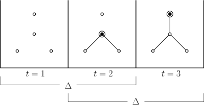
Figure 1: A minimum-cardinality sliding $\Delta$-window temporal vertex cover which selects a vertex appearance at time step $t=3$, whose corresponding vertex belongs in no minimum vertex cover of $G_{3}$.

5 Approximation hardness of 2-TVC

In this section we study the complexity of $\Delta$-TVC  where $\Delta$ is constant. We start with an intuitive observation that, for every fixed $\Delta$, the problem ($\Delta+1$)-TVC is at least as hard as $\Delta$-TVC. Indeed, let $\mathcal{A}$ be an algorithm that computes a minimum-cardinality sliding $(\Delta+1)$-window temporal vertex cover of $(G,\lambda)$. It is easy to see that a minimum-cardinality sliding $\Delta$-window temporal vertex cover of $(G,\lambda)$ can also be computed using $\mathcal{A}$, if we amend the input temporal graph by inserting one edgeless snapshot after every $\Delta$ consecutive snapshots of $(G,\lambda)$, see Figure 2.

Figure 2: Inserting “empty” time slots to compute a minimum-cardinality sliding $\Delta$-window temporal vertex cover on $(G,\lambda)$ using algorithm $\mathcal{A}$ for ($\Delta+1$)-TVC.

Since the $1$-TVC problem is equivalent to solving $T$ instances of Vertex Cover (on static graphs), the above reduction demonstrates in particular that, for any natural $\Delta$, $\Delta$-TVC is at least as hard as Vertex Cover. Therefore, if Vertex Cover is hard for a class $\mathcal{X}$ of static graphs, then $\Delta$-TVC is also hard for the class of always $\mathcal{X}$ temporal graphs. In this section, we show that the converse is not true. Namely, we reveal a class $\mathcal{X}$ of graphs, for which Vertex Cover can be solved in linear time, but 2-TVC is NP-hard on always $\mathcal{X}$ temporal graphs. In fact, we show the even stronger result that 2-TVC does not admit a PTAS on always $\mathcal{X}$ temporal graphs, unless P=NP.

To prove the main result (in Theorem 10) we start with an auxiliary lemma, showing that, unless P=NP, Vertex Cover does not admit a PTAS on the class $\mathcal{Z}$ of graphs which can be obtained from a cubic graph by subdividing every edge exactly 4 times.

Lemma 2.

Vertex Cover on $\mathcal{Z}$ does not admit a PTAS, unless P=NP.

Proof.

Vertex Cover does not admit a PTAS when the input is restricted to be a cubic graph, unless P=NP[7]. By a simple reduction we will show that Vertex Cover still does not admit a PTAS when the input is restricted to be a graph that belongs to the class $\mathcal{Z}$, i.e. a graph obtained from a cubic graph by subdividing every edge exactly 4 times. For an illustration we refer to Figure 4, in which the first graph $K_{4}$ is the cubic graph on four vertices and the second graph is the graph obtained from $K_{4}$ by subdividing every edge 4 times.

Given a cubic graph $G$, let $H\in\mathcal{Z}$ be the graph obtained from $G$ by subdividing each edge 4 times. It is well known and can be easily verified that a double subdivision of an edge increases the size of a minimum vertex cover exactly by one. Hence, denoting by $\tau(G)$ and $\tau(H)$ the sizes of minimum vertex covers of $G$ and $H$, respectively, we have:

$$\tau(H)=\tau(G)+2m,$$ (5)

where $m$ is the number of edges in $G$.

Now we will prove that, starting from an arbitrary (not necessarily optimum) vertex cover $S_{H}$ for $H$, we can efficiently compute a vertex cover $S_{G}$ for $G$ of size $|S_{G}|\leq|S_{H}|-2m$. To this end, we show how to construct $S_{G}$ from $S_{H}$ by decreasing the cardinality of $S_{H}$ by at least two for every edge of $G$. Initially, we set $S_{G}=S_{H}$. Let $uv\in E(G)$ be an edge in $G$, and let $ua_{1},a_{1}a_{2},a_{2}a_{3},a_{3}a_{4},a_{4}v$ be the edges of $H$ that correspond to the 4-subdivision of $uv$. Note that $S_{H}$ contains at least two of the vertices $a_{1},a_{2},a_{3},a_{4}$. Suppose that at least one of the vertices $u,v$ is contained in $S_{H}$. Then we just remove from $S_{G}$ all its vertices among $\{a_{1},a_{2},a_{3},a_{4}\}$. Suppose otherwise that none of $u,v$ is contained in $S_{H}$. Then it is easy to verify that $S_{H}$ contains at least three of the vertices $a_{1},a_{2},a_{3},a_{4}$. In this case, we add $u$ to $S_{G}$ and we remove from $S_{G}$ all its vertices among $\{a_{1},a_{2},a_{3},a_{4}\}$. After repeating this procedure for every edge of $G$, we obtain a set $S_{G}$ that still covers all edges of $G$, while $|S_{G}|\leq|S_{H}|-2m$ holds.

To complete the proof, suppose for the sake of contradiction that there exists a PTAS for Vertex Cover in $\mathcal{Z}$. That is, for every $\epsilon>0$, we can compute in polynomial time a vertex cover $S_{H}$ of $H$ such that $|S_{H}|\leq(1+\epsilon)\tau(H)$. As we showed above, starting from $S_{H}$, we can compute in polynomial time a vertex cover $S_{G}$ of $G$ such that

$$\begin{split}|S_{G}|&\leq|S_{H}|-2m\\ &\leq(1+\epsilon)\tau(H)-2m\\ &=(1+\epsilon)(\tau(G)+2m)-2m\\ &=(1+\epsilon)\tau(G)+2\epsilon\cdot m\\ &\leq(1+\epsilon)\tau(G)+6\epsilon\cdot\tau(G)\\ &=(1+7\epsilon)\tau(G),\end{split}$$ (6)

where in the first equality we used (5), and in the last inequality we used the fact that $m\leq 3\tau(G)$, because every vertex in the cubic graph $G$ covers exactly 3 edges. Summarizing, the existence of a PTAS for Vertex Cover in the class $\mathcal{Z}$ would imply the existence of a PTAS in the class of cubic graphs, which is a contradiction, unless P=NP [7]. ∎

Let now $\mathcal{X}$ be the class of graphs whose connected components are induced subgraphs of graph $\Psi$ (see Figure 1). Clearly, Vertex Cover is linearly solvable on graphs from $\mathcal{X}$. We will show that, unless P=NP, 2-TVC does not admit a PTAS on always $\mathcal{X}$ temporal graphs by using a reduction from Vertex Cover on $\mathcal{Z}$.

Figure 3: The graph $\Psi$.

Theorem 10.

2-TVC on always $\mathcal{X}$ temporal graphs does not admit a PTAS, unless P=NP.

Proof.

To prove the theorem we will reduce Vertex Cover on $\mathcal{Z}$ to 2-TVC on always $\mathcal{X}$ temporal graphs. Let $H=(V,E)$ be a graph in $\mathcal{Z}$. First we will show how to construct an always $\mathcal{X}$ temporal graph $(G,\lambda)$ of lifetime 2. Then we will prove that the size $\tau$ of a minimum vertex cover of $H$ is equal to the size $\sigma$ of a minimum-cardinality sliding 2-window temporal vertex cover of $(G,\lambda)$.

Let $R\subseteq V$ be the set of vertices of degree 3 in $H$. We define $(G,\lambda)$ to be a temporal graph of lifetime 2, where snapshot $G_{1}$ is obtained from $H$ by removing the edges with both ends being at distance exactly 2 from $R$, and snapshot $G_{2}=H-R$. Figure 4 illustrates the reduction for $H=K_{4}$.

Let $\mathcal{S}=(S_{1},1)\cup(S_{2},2)$ be an arbitrary sliding 2-window temporal vertex cover of $(G,\lambda)$ for some $S_{1},S_{2}\subseteq V$. Since every edge of $H$ belongs to at least one of the graphs $G_{1}$ and $G_{2}$, the set $S_{1}\cup S_{2}$ covers all the edges of $H$. Hence, $\tau\leq|S_{1}\cup S_{2}|\leq|S_{1}|+|S_{2}|=|\mathcal{S}|$. As $\mathcal{S}$ was chosen arbitrarily we further conclude that $\tau\leq\sigma$.

To show the converse inequality, let $C\subseteq V$ be a minimum vertex cover of $H$. Let $S_{1}$ be those vertices in $C$ which either have degree 3, or have a neighbor of degree 3. Let also $S_{2}=C\setminus S_{1}$. We claim that $(S_{1},1)\cup(S_{2},2)$ is a sliding 2-window temporal vertex cover of $(G,\lambda)$. First, let $e\in E$ be an edge in $H$ incident to a vertex of degree 3. Then, by the construction, $e$ is active only in time slot 1, i.e. $e\in E_{1}\setminus E_{2}$, and a vertex $v$ in $C$ covering $e$ belongs to $S_{1}$. Hence, $e$ is temporally covered by $(v,1)$ in $(G,\lambda)$. Let now $e\in E$ be an edge in $H$ whose both end vertices have degree 2. If one of the end vertices of $e$ is adjacent to a vertex of degree 3 in $H$, then, by the construction, $e$ is active in both time slots $1$ and $2$. Therefore, since $C=S_{1}\cup S_{2}$, edge $e$ will be temporally covered in $(G,\lambda)$ in at least one of the time slots. Finally, if none of the end vertices of $e$ is adjacent to a vertex of degree 3 in $H$, then $e$ is active only in time slot 2, i.e. $e\in E_{2}\setminus E_{1}$. Moreover, by the construction a vertex $v$ in $C$ covering $e$ belongs to $S_{2}$. Hence, $e$ is temporally covered by $(v,2)$ in $(G,\lambda)$. This shows that $(S_{1},1)\cup(S_{2},2)$ is a sliding 2-window temporal vertex cover of $(G,\lambda)$, and thus $\sigma\leq|S_{1}|+|S_{2}|=|C|=\tau$. Therefore $\sigma=\tau$.

Note that for any $r\in\mathbb{N}$, any feasible solution of 2-TVC on $(G,\lambda)$ with size $r$ defines a vertex cover of $H$ with size at most $r$. Therefore, since $\sigma=\tau$ as we proved above, any PTAS for 2-TVC on always $\mathcal{X}$ temporal graphs implies a PTAS for Vertex Cover in the class $\mathcal{Z}$, which is a contradiction by Lemma 2, unless P=NP. ∎

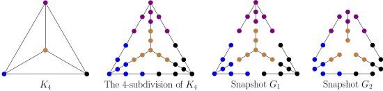
Figure 4: A cubic graph $K_{4}$, its 4-subdivision, and the corresponding snapshots $G_{1}$ and $G_{2}$

6 Approximation algorithms

In this section we provide several approximation algorithms for SW-TVC. The approximation factors that we achieve depend on various parameters of the input temporal graph. The values of these parameters (and of the corresponding approximation factors) are in general incomparable to each other, and thus the best option for approximating the optimal solution depends on the values of those parameters in each specific input instance.

6.1 Approximations in terms of $T$, $\Delta$, and the largest edge frequency

We begin by presenting a reduction from SW-TVC to Set Cover, which proves useful for deriving approximation algorithms for the original problem. We note here the similarity of the construction in this reduction to the construction in the reduction of TVC to Set Cover presented in Theorem 4. Consider an instance, $(G,\lambda)$ and $\Delta\leq T$, of the SW-TVC problem. Construct an instance of Set Cover as follows: Let the universe be $U=\{(e,t):e\in E[W_{t}],t\in[1,T-\Delta+1]\}$, i.e. the set of all pairs $(e,t)$ of an edge $e$ and a time slot $t$ such that $e$ appears (and so must be temporally covered) within window $W_{t}$. For every vertex appearance $(v,s)$ we define $C_{v,s}$ to be the set of elements $(e,t)$ in the universe $U$, such that $(v,s)$ temporally covers $e$ in the window $W_{t}$. Formally, $C_{v,s}=\{(e,t):v\text{ is an endpoint of }e,e\in E_{s},\text{ and }s\in W_{t}\}$. Let $\mathcal{C}$ be the family of all sets $C_{v,s}$, where $v\in V,s\in[1,T]$. The following lemma shows that finding a minimum-cardinality sliding $\Delta$-window temporal vertex cover of $(G,\lambda)$ is equivalent to finding a minimum-cardinality family of sets $C_{v,s}$ that covers the universe $U$.

Lemma 3.

A family $\mathcal{C}=\{C_{v_{1},t_{1}},\ldots,C_{v_{k},t_{k}}\}$ is a set cover of $U$ if and only if $\mathcal{S}=\{(v_{1},t_{1}),\ldots,(v_{k},t_{k})\}$ is a sliding $\Delta$-window temporal vertex cover of $(G,\lambda)$.

Proof.

First assume that $\mathcal{C}$ is a set cover of $U$, but $\mathcal{S}$ is not a sliding $\Delta$-window temporal vertex cover of $(G,\lambda)$. Then there exists a window $W_{r}$ for some $r\in[1,T-\Delta+1]$, such that an edge $uv$ appears in $W_{r}$ but is not temporally covered in $W_{r}$ by $\mathcal{S}$. This means that, for every $j\in W_{r}$ such that $uv\in E_{j}$, neither $(u,j)$ nor $(v,j)$ belongs to $\mathcal{S}$. Therefore, $C_{u,j},C_{v,j}\notin\mathcal{C}$ for all $j\in W_{r}$ such that $uv\in E_{j}$. But then $\mathcal{C}$ does not cover $(uv,r)\in U$, which is a contradiction.

Conversely, assume that $\mathcal{S}$ is a sliding $\Delta$-window temporal vertex cover of $(G,\lambda)$, but $\mathcal{C}$ is not a set cover of $U$, i.e. there exists some $(uv,r)\in U$ which belongs to none of the sets in $\mathcal{C}$. The latter means that $C_{u,j},C_{v,j}\notin\mathcal{C}$, and therefore $(u,j),(v,j)\notin\mathcal{S}$, for every $j\in W_{r}$ such that $uv\in E_{j}$. Therefore $uv$ is not covered in $W_{r}$, which is a contradiction. ∎

$(\ln{n}+\ln{\Delta}+\frac{1}{2})$-approximation.

In the instance of Set Cover constructed by the above reduction, every set $C_{v,s}$ in $\mathcal{C}$ contains at most $n\Delta$ elements of the universe $U$. Indeed, the vertex appearance $(v,s)$ temporally covers at most $n-1$ edges, each in at most $\Delta$ windows (namely from window $W_{s-\Delta+1}$ up to window $W_{s}$). Thus we can apply the polynomial-time greedy algorithm of [14] for Set Cover which achieves an approximation ratio of $H_{n\Delta}-\frac{1}{2}$, where $n\Delta$ is the maximum size of a set in the input instance and $H_{n\Delta}=\sum_{i=1}^{n\Delta}\frac{1}{i}\leq\ln{n}+\ln{\Delta}+1$ is the $n\Delta$-th harmonic number.

$2k$-approximation, where $k$ is the maximum edge frequency.

Given a temporal graph $(G,\lambda)$ and an edge $e$ of $G$, the $\Delta$-frequency of $e$ is the maximum number of time slots at which $e$ appears within a $\Delta$-window. Let $k$ denote the maximum $\Delta$-frequency over all edges of $G$. Clearly, for a particular $\Delta$-window $W_{t}$, an edge $e\in E[W_{t}]$ can be temporally covered in $W_{t}$ by at most $2k$ vertex appearances. So in the above reduction to Set Cover, every element $(e,t)\in U$ belongs to at most $2k$ sets in $\mathcal{C}$. Therefore, the optimal solution of the constructed instance of Set Cover can be approximated within a factor of $2k$ in polynomial time [45, p. 118-9], yielding a polynomial-time $2k$-approximation for SW-TVC.

$2\Delta$-approximation.

Since the maximum $\Delta$-frequency of an edge is always upper-bounded by $\Delta$, the previous algorithm gives a worst-case polynomial-time $2\Delta$-approximation for SW-TVC on arbitrary temporal graphs.

6.2 Approximation in terms of maximum degree of snapshots

In this section we give a polynomial-time $d$-approximation algorithm for the SW-TVC problem on always degree at most $d$ temporal graphs, that is, on temporal graphs where the maximum degree in each snapshot is at most $d$. In particular, the algorithm computes an optimum solution (i.e. with approximation ratio $d=1$) for always matching (i.e. always degree at most $1$) temporal graphs. As a building block, we first provide an exact $O(T)$-time algorithm for optimally solving SW-TVC in the class of single-edge temporal graphs, namely temporal graphs whose underlying graph is a single edge. To that end, we reduce SW-TVC to Interval Covering, leading to an intuitive algorithm which selects the “rightmost” appearance of the edge of the temporal graph within a time window in which the edge has not been covered yet (starting from the first time window). In fact, this algorithm is a direct translation of a known greedy algorithm which solves Interval Covering in the SW-TVC single-edge-temporal-graphs setting. Once we have established this exact algorithm for single-edge temporal graphs, we prove that for always degree at most $d$ temporal graphs we can $d$-approximate the optimal solution by independently solving SW-TVC for every single-edge temporal subgraph and then taking the union of these solutions.

Single-edge temporal graphs

Consider a temporal graph $(G_{0},\lambda)$ where $G_{0}$ is the single-edge graph, i.e. $V(G_{0})=\{u,v\}$ and $E(G_{0})=\{uv\}$. We reduce SW-TVC on $(G_{0},\lambda)$ to an instance of Interval Covering, which has a known greedy algorithm that we then translate to an algorithm for SW-TVC on single-edge temporal graphs.

Interval Covering Input: A family $\mathcal{I}$ of intervals in the line. Output: A minimum-cardinality subfamily $\mathcal{I}^{\prime}\subseteq\mathcal{I}$ such that $\bigcup_{I\in\mathcal{I}}=\bigcup_{I\in\mathcal{I}^{\prime}}$.

We construct the family $\mathcal{I}$ as follows. For every $i=1,2,\ldots,T$ such that $uv\in E_{i}$ we include into $\mathcal{I}$ the interval $I_{i}=[i-\Delta+1,i]\cap[1,T-\Delta+1]$, which contains the first time slot of each of those $\Delta$-windows that include time slot $i$.

Lemma 4.

Let $i_{1},i_{2},\ldots,i_{k}$ be such that $uv\in E_{i_{j}}$ for every $j=1,2,\ldots,k$. Then $\mathcal{I}^{\prime}=\{I_{i_{1}},\ldots,I_{i_{k}}\}$ is an interval covering of $\mathcal{I}$ if and only if $\mathcal{S}=\{(u,i_{1}),(u,i_{2}),\ldots,(u,i_{k})\}$ is a sliding $\Delta$-window temporal vertex cover of $(G_{0},\lambda)$.

Proof.

Assume first that $\mathcal{I}^{\prime}$ is an interval covering of $\mathcal{I}$, but $\mathcal{S}$ is not a sliding $\Delta$-window temporal vertex cover of $(G_{0},\lambda)$. The latter means that there exists a $\Delta$-window $W_{t}$ such that $uv$ exists at some time slot $s$ in $W_{t}$, but $uv$ is not temporally covered by any vertex appearance in $\mathcal{S}[W_{t}]$. Therefore $t\notin I_{i_{1}}\cup I_{i_{2}}\cup\ldots\cup I_{i_{k}}$, but $t\in I_{s}$, which contradicts the assumption that $\mathcal{I}^{\prime}$ is an interval covering of $\mathcal{I}$.

Conversely, assume that $\mathcal{S}$ a sliding $\Delta$-window temporal vertex cover of $(G_{0},\lambda)$, but $\mathcal{I}^{\prime}$ is not an interval covering of $\mathcal{I}$, that is, there exists $I_{i}\in\mathcal{I}$ and $t\in I_{i}$ such that $t\notin\bigcup_{I\in\mathcal{I}^{\prime}}I$. By the construction, this means that $uv\in E_{i}$ is not temporally covered by any vertex appearances in $\mathcal{S}[W_{t}]$, which is a contradiction. ∎

Lemma 4 shows that finding a minimum-cardinality sliding $\Delta$-window temporal vertex cover of $(G_{0},\lambda)$ is equivalent to finding a minimum interval covering of $\mathcal{I}$. An easy linear-time greedy algorithm for the Interval Covering picks at each iteration, among the intervals that cover the leftmost uncovered point, the one with largest finishing time. Algorithm 2 implements this simple rule in the context of the SW-TVC problem.

Algorithm 2 SW-TVC on single-edge temporal graphs

0:  A temporal graph $(G_{0},\lambda)$ of lifetime $T$ with $V(G_{0})=\{u,v\}$, and $\Delta\leq T$.

0:  A minimum-cardinality sliding $\Delta$-window temporal vertex cover $\mathcal{S}$ of $(G_{0},\lambda)$.

1:  $\mathcal{S}\leftarrow\emptyset$

2:  $t=1$

3:  while $t\leq T-\Delta+1$ do

4:     if $\exists r\in[t,t+\Delta-1]$ such that $uv\in E_{r}$ then

5:        choose maximum such $r$ and add $(u,r)$ to $\mathcal{S}$

6:        $t\leftarrow r+1$

7:     else

8:        $t\leftarrow t+1$

9:  return  $\mathcal{S}$

Lemma 5.

Algorithm 2 solves SW-TVC on a single-edge temporal graph and can be implemented to work in time $O\left(T\right)$.

Proof.

The time complexity of the algorithm is dominated by the running time of the while-loop. We provide an implementation of the while-loop, which works in time $O(T)$: in each iteration, we inspect the current $\Delta$-window $[t,t+\Delta-1]$ from the rightmost time slot moving to the left. As we go through the time slots, we mark the ones in which edge $uv$ does not appear as “NO”. When we move to the next iteration (the next $\Delta$-window), we do not need to revisit any time slots that have been marked as “NO” and we immediately move to the next iteration whenever we meet such a slot. This way we visit every time slot at most once, and hence we exit the while-loop after $O(T)$ operations. ∎

Always degree at most $d$ temporal graphs

We present now the main algorithm of this section, the idea of which is to independently solve SW-TVC for every possible single-edge temporal subgraph of a given temporal graph by Algorithm 2, and take the union of these solutions. We will show that this algorithm is a $d$-approximation algorithm for SW-TVC on always degree at most $d$ temporal graphs.

Let $(G,\lambda)$ be a temporal graph, where $G=(V,E)$, $|V|=n$, and $|E|=m$. For every edge $e=uv\in E$, let $(G[\{u,v\}],\lambda)$ denote the temporal graph where the underlying graph is the induced subgraph $G[\{u,v\}]$ of $G$ and the labels of $e$ are exactly the same as in $(G,\lambda)$.

Algorithm 3 $d$-approximation of SW-TVC on always degree at most $d$ temporal graphs

0:  An always degree at most $d$ temporal graph $(G,\lambda)$ of lifetime $T$, and $\Delta\leq T$.

0:  A sliding $\Delta$-window temporal vertex cover $\mathcal{S}$ of $(G,\lambda)$.

1:  for $i=1$ to $T$ do

2:     $\mathcal{S}_{i}\leftarrow\emptyset$

3:  for every edge $e=uv\in E(G)$ do

4:     Compute the optimal solution $\mathcal{S}^{e}$ of the problem for $(G[\{u,v\}],\lambda)$ by Algorithm 2

5:     for $i=1$ to $T$ do

6:        $\mathcal{S}_{i}\leftarrow\mathcal{S}_{i}\cup\mathcal{S}^{e}_{i}$

7:  return  $\mathcal{S}$

Lemma 6.

Algorithm 3 is a $O\left(mT\right)$-time $d$-approximation algorithm for SW-TVC on always degree at most $d$ temporal graphs.

Proof.

Let $(G,\lambda)$ be an always degree at most $d$ temporal graph of lifetime $T$, and let $\mathcal{S}^{*}$ be a minimum-cardinality sliding $\Delta$-window temporal vertex cover of $(G,\lambda)$. We will show that $|\mathcal{S}|\leq d\cdot|\mathcal{S}^{*}|$, where $\mathcal{S}$ is the solution computed by Algorithm 3. To this end we apply a double counting argument to the set $C$ of all triples $(v,e,t)\in V\times E\times[1,T]$ such that $v\in\mathcal{S}^{*}_{t}$, $e\in E_{t}$, and $v$ is incident to $e$.

On the one hand

$$|C|=\sum\limits_{t=1}^{T}\sum\limits_{v\in\mathcal{S}^{*}_{t}}|\{(v,e,t):e\in E_{t}\text{ and $v$ is incident to $e$}\}|\leq\sum\limits_{t=1}^{T}\sum\limits_{v\in\mathcal{S}^{*}_{t}}d=d\cdot|\mathcal{S}^{*}|,$$

where the inequality follows from the assumption that every snapshot of $(G,\lambda)$ has maximum degree at most $d$.

On the other hand

$$|C|=\sum\limits_{e\in E}\sum\limits_{t=1}^{T}|\{(v,e,t):e\in E_{t},v\in\mathcal{S}^{*}_{t},\text{ and $v$ is incident to $e$}\}|\geq\sum\limits_{e\in E}|\mathcal{S}^{e}|=|\mathcal{S}|,$$

where $\mathcal{S}^{e}$ is the optimum sliding $\Delta$-window temporal vertex cover of the temporal graph $(G[\{u,v\}],\lambda)$ (see line 4 of Algorithm 3). The last inequality follows from the fact that the restriction of any sliding $\Delta$-window temporal vertex cover of $(G,\lambda)$ to the temporal subgraph induced by the endpoints of $e$ is a sliding $\Delta$-window temporal vertex cover of the temporal subgraph, and therefore has cardinality at least $|\mathcal{S}^{e}|$. We conclude that $|\mathcal{S}|\leq|C|\leq d\cdot|\mathcal{S}^{*}|$, as required.

The time-complexity of Algorithm 3 is dominated by the time needed to execute the for-loop of lines 3-6. The latter requires time $O\left(mT\right)$. ∎

Note that in the case of always matching temporal graphs, i.e. where every snapshot is a matching, the maximum degree in each snapshot is $d=1$, so the above $d$-approximation actually yields an exact algorithm (see Corollary 1). This is not surprising, since a single vertex appearance can only cover one edge in always matching temporal graphs. Therefore, the solutions for different edges can be independently optimized.

Corollary 1.

SW-TVC can be optimally solved in $O(mT)$ time on the class of always matching temporal graphs.

7 Conclusions and open problems

In this paper we introduced and studied two natural temporal extensions of the problem Vertex Cover for static graphs, namely Temporal Vertex Cover and Sliding Window Temporal Vertex Cover (for short, TVC and SW-TVC, respectively), which take into account the dynamic nature of temporal networks. We presented a thorough investigation of the complexity and approximability of these problems, including strong hardness results, and various approximation and exact algorithms. In particular, for SW-TVC we designed a linear-time optimal algorithm on always degree at most 1 temporal graphs, i.e. on temporal graphs that consist of a matching in each time step. On the other hand, we showed that SW-TVC becomes NP-hard on always degree at most 3 temporal graphs, even when the underlying graph is cubic and every snapshot has connected components with at most 7 vertices. This leaves an intriguing open question of the complexity status of the problem on always degree at most 2 temporal graphs, i.e. on temporal graphs that consist of disjoint paths and cycles in each time step.

Problem 1.

Restricted on always degree at most 2 temporal graphs, is SW-TVC efficiently solvable?

For SW-TVC we provided various polynomial-time approximation algorithms, including a $2\Delta$-approximation algorithm for general temporal graphs, and a $d$-approximation algorithm for always degree at most $d$ temporal graphs. There are no known matching lower bounds for these approximation factors, and it would be interesting to know whether there is any room for improvement.

Problem 2.

Let $d$ be the maximum vertex degree in each snapshot of a temporal graph. Can SW-TVC be efficiently approximated within a factor better than $2\Delta$ or better than $d$? In particular, does there exist a polynomial-time approximation algorithm for SW-TVC with approximation factor $o(\Delta)$ or $o(d)$?

A natural extension of the problem SW-TVC is computing a sliding $\Delta$-window temporal vertex cover that minimizes the maximum cost (i.e. the maximum number of vertex appearances) over all time windows of a given length $\ell\geq\Delta$. Formally this problem can be defined as follows.

Restricted-Length Sliding Window Temporal Vertex Cover   (RL-SW-TVC) Input: A temporal graph $(G,\lambda)$ with lifetime $T$, and two integers $\Delta\leq\ell\leq T$. Output: A sliding $\Delta$-window temporal vertex cover $\mathcal{S}$ of $(G,\lambda)$ such that the number of vertex appearances of $\mathcal{S}$ in any time window of length $\ell$ is minimized.

Clearly, SW-TVC is the special case of RL-SW-TVC where $\ell=T$, in which case we aim at minimizing the total number of vertex appearances in the solution. Although the two problems might look superficially similar to each other, they are different, as we illustrate in the example of Figure 5, where $T=3$ and $\ell=\Delta=2$. Figure 5 an optimal solution to SW-TVC is highlighted, which contains in total 4 vertex appearances (all at time $t=2$). In this solution, the maximum number of vertex appearances in every time window of length $\ell=2$ is 4. On the other hand, Figure 5 an optimal solution to RL-SW-TVC for $\ell=2$ is highlighted, which contains in total 5 vertex appearances. In this solution, the maximum number of vertex appearances in every time window of length $\ell=2$ is 3.

Problem 3.

Is the problem RL-SW-TVC strictly harder than SW-TVC? Can our results be extended to RL-SW-TVC?

Figure 5: A temporal graph $(G,\lambda)$ with lifetime $T=3$, where $\Delta=2$. (a) An optimal solution to SW-TVC and (b) an optimal solution to RL-SW-TVC where $\ell=\Delta=2$.

Finally, it will be interesting to investigate the practical aspects of the studied problems, TVC and SW-TVC, and in particular to practically evaluate the performance of the different presented algorithms on real-world instances.

Problem 4.

How do the different approximation and exact algorithms perform on real-world temporal graph instances?

References

- [1] E. Aaron, D. Krizanc, and E. Meyerson. DMVP: foremost waypoint coverage of time-varying graphs. In Proceedings of the 40th International Workshop on Graph-Theoretic Concepts in Computer Science (WG), pages 29–41, 2014.
- [2] E. C. Akrida, L. Gasieniec, G. B. Mertzios, and P. G. Spirakis. Ephemeral networks with random availability of links: The case of fast networks. Journal of Parallel and Distributed Computing, 87:109–120, 2016.
- [3] E. C. Akrida, L. Gasieniec, G. B. Mertzios, and P. G. Spirakis. The complexity of optimal design of temporally connected graphs. Theory of Computing Systems, 61(3):907–944, 2017.
- [4] E. C. Akrida, G. B. Mertzios, S. Nikoletseas, C. Raptopoulos, P. G. Spirakis, and V. Zamaraev. How fast can we reach a target vertex in stochastic temporal graphs? In Proceedings of the 46th International Colloquium on Automata, Languages and Programming (ICALP), pages 131:1–131:14, 2019.
- [5] E. C. Akrida, G. B. Mertzios, and P. G. Spirakis. The temporal explorer who returns to the base. In Proceedings of the 11th International Conference on Algorithms and Complexity (CIAC ’19), pages 13–24, 2019.
- [6] E. C. Akrida, G. B. Mertzios, P. G. Spirakis, and V. Zamaraev. Temporal vertex covers and sliding time windows. In Proceedings of the 45th International Colloquium on Automata, Languages, and Programming (ICALP), pages 148:1–148:14, 2018.
- [7] P. Alimonti and V. Kann. Some APX-completeness results for cubic graphs. Theoretical Computer Science, 237(1-2):123–134, 2000.
- [8] J. Baste, B.-M. Bui-Xuan, and A. Roux. Temporal matching. Theoretical Computer Science, 2019.
- [9] B.-M. Bui-Xuan, A. Ferreira, and A. Jarry. Computing shortest, fastest, and foremost journeys in dynamic networks. International Journal of Foundations of Computer Science, 14(2):267–285, 2003.
- [10] A. Casteigts and P. Flocchini. Deterministic Algorithms in Dynamic Networks: Formal Models and Metrics. Technical report, Defence R&D Canada, April 2013.
- [11] A. Casteigts and P. Flocchini. Deterministic Algorithms in Dynamic Networks: Problems, Analysis, and Algorithmic Tools. Technical report, Defence R&D Canada, April 2013.
- [12] A. Casteigts, P. Flocchini, W. Quattrociocchi, and N. Santoro. Time-varying graphs and dynamic networks. International Journal of Parallel, Emergent and Distributed Systems, 27(5):387–408, 2012.
- [13] A. Casteigts, B. Mans, and L. Mathieson. On the feasibility of maintenance algorithms in dynamic graphs, 2011. Technical Report available at http://arxiv.org/abs/1107.2722.
- [14] R. chii Duh and M. Fürer. Approximation of -set cover by semi-local optimization. In Proceedings of the 29th Annual ACM Symposium on Theory of Computing (STOC), pages 256–264, 1997.
- [15] A. E. F. Clementi, C. Macci, A. Monti, F. Pasquale, and R. Silvestri. Flooding time of edge-markovian evolving graphs. SIAM Journal on Discrete Mathematics, 24(4):1694–1712, 2010.
- [16] M. Cygan, H. Dell, D. Lokshtanov, D. Marx, J. Nederlof, Y. Okamoto, R. Paturi, S. Saurabh, and M. Wahlström. On problems as hard as CNF-SAT. ACM Transactions on Algorithms, 12(3):41:1–41:24, 2016.
- [17] S. Dobrev, S. Durocher, M. E. Hesari, K. Georgiou, E. Kranakis, D. Krizanc, L. Narayanan, J. Opatrny, S. M. Shende, and J. Urrutia. Complexity of barrier coverage with relocatable sensors in the plane. Theoretical Computer Science, 579:64–73, 2015.
- [18] J. Enright, K. Meeks, G. B. Mertzios, and V. Zamaraev. Deleting edges to restrict the size of an epidemic in temporal networks, 2018. Technical Report available at http://arxiv.org/abs/1805.06836.
- [19] T. Erlebach, M. Hoffmann, and F. Kammer. On temporal graph exploration. In Proceedings of the 42nd International Colloquium on Automata, Languages, and Programming (ICALP), pages 444–455, 2015.
- [20] U. Feige. A threshold of for approximating set cover. Journal of the ACM, 45(4):634–652, 1998.
- [21] A. Ferreira. Building a reference combinatorial model for MANETs. IEEE Network, 18(5):24–29, 2004.
- [22] P. Flocchini, B. Mans, and N. Santoro. Exploration of periodically varying graphs. In Proceedings of the 20th International Symposium on Algorithms and Computation (ISAAC), pages 534–543, 2009.
- [23] M. R. Garey and D. S. Johnson. Computers and intractability: A guide to the theory of NP-completeness. W. H. Freeman & Co., New York, NY, USA, 1979.
- [24] G. Giakkoupis, T. Sauerwald, and A. Stauffer. Randomized rumor spreading in dynamic graphs. In Proceedings of the 41st International Colloquium on Automata, Languages and Programming (ICALP), pages 495–507, 2014.
- [25] M. E. Hesari, E. Kranakis, D. Krizanc, O. M. Ponce, L. Narayanan, J. Opatrny, and S. M. Shende. Distributed algorithms for barrier coverage using relocatable sensors. Distributed Computing, 29(5):361–376, 2016.
- [26] A. Himmel, H. Molter, R. Niedermeier, and M. Sorge. Adapting the bron-kerbosch algorithm for enumerating maximal cliques in temporal graphs. Social Network Analysis and Mining, 7(1):35:1–35:16, 2017.
- [27] P. Holme and J. Saramäki, editors. Temporal Networks. Springer, 2013.
- [28] R. Impagliazzo and R. Paturi. On the complexity of -SAT. Journal of Computer and System Sciences, 62(2):367–375, 2001.
- [29] R. Impagliazzo, R. Paturi, and F. Zane. Which problems have strongly exponential complexity? Journal of Computer and System Sciences, 63(4):512–530, 2001.
- [30] D. Kempe, J. M. Kleinberg, and A. Kumar. Connectivity and inference problems for temporal networks. In Proceedings of the 32nd annual ACM symposium on Theory of computing (STOC), pages 504–513, 2000.
- [31] O. Kostakis and A. Gionis. On mining temporal patterns in dynamic graphs, and other unrelated problems. In Proceedings of the 6th International Conference on Complex Networks and Their Applications (COMPLEX NETWORKS), pages 516–527, 2017.
- [32] O. Kostakis, N. Tatti, and A. Gionis. Discovering recurring activity in temporal networks. Data Mining and Knowledge Discovery, 31(6):1840–1871, 2017.
- [33] E. Kranakis, D. Krizanc, F. L. Luccio, and B. Smith. Maintaining intruder detection capability in a rectangular domain with sensors. In Proceedings of the 11th International Symposium on Algorithms and Experiments for Wireless Sensor Networks (ALGOSENSORS), pages 27–40, 2015.
- [34] J. Leskovec, J. M. Kleinberg, and C. Faloutsos. Graph evolution: Densification and shrinking diameters. ACM Transactions on Knowledge Discovery from Data, 1(1), 2007.
- [35] D. Lokshtanov, D. Marx, and S. Saurabh. Lower bounds based on the Exponential Time Hypothesis. Bulletin of the EATCS, pages 41–71, 2011.
- [36] G. B. Mertzios, O. Michail, I. Chatzigiannakis, and P. G. Spirakis. Temporal network optimization subject to connectivity constraints. Algorithmica, pages 1416–1449, 2019.
- [37] G. B. Mertzios, H. Molter, R. Niedermeier, V. Zamaraev, and P. Zschoche. Computing maximum matchings in temporal graphs, 2019. Technical Report available at https://arxiv.org/abs/1905.05304.
- [38] G. B. Mertzios, H. Molter, and V. Zamaraev. Sliding window temporal graph coloring. In Proceedings of the 33rd AAAI Conference on Artificial Intelligence (AAAI), pages 7667–7674, 2019.
- [39] O. Michail and P. G. Spirakis. Traveling salesman problems in temporal graphs. Theoretical Computer Science, 634:1–23, 2016.
- [40] O. Michail and P. G. Spirakis. Elements of the theory of dynamic networks. Communications of the ACM, 61(2):72–72, Jan. 2018.
- [41] R. Niedermeier and P. Rossmanith. An efficient fixed-parameter algorithm for 3-hitting set. Journal of Discrete Algorithms, 1(1):89–102, 2003.
- [42] S. E. Nikoletseas and P. G. Spirakis. Probabilistic distributed algorithms for energy efficient routing and tracking in wireless sensor networks. Algorithms, 2(1):121–157, 2009.
- [43] P. Rozenshtein, N. Tatti, and A. Gionis. The network-untangling problem: From interactions to activity timelines. In Proceedings of the Joint European Conference on Machine Learning and Knowledge Discovery in Databases, pages 701–716, 2017.
- [44] J. K. Tang, M. Musolesi, C. Mascolo, and V. Latora. Characterising temporal distance and reachability in mobile and online social networks. ACM Computer Communication Review, 40(1):118–124, 2010.
- [45] V. V. Vazirani. Approximation algorithms. Springer, 2003.
- [46] J. Viard, M. Latapy, and C. Magnien. Revealing contact patterns among high-school students using maximal cliques in link streams. In Proceedings of the 2015 IEEE/ACM International Conference on Advances in Social Networks Analysis and Mining (ASONAM), pages 1517–1522, 2015.
- [47] T. Viard, M. Latapy, and C. Magnien. Computing maximal cliques in link streams. Theoretical Computer Science, 609:245–252, 2016.
- [48] C. Zhu, C. Zheng, L. Shu, and G. Han. A survey on coverage and connectivity issues in wireless sensor networks. Journal of Network and Computer Applications, 35(2):619–632, 2012.