Stroke Controllable Fast Style Transfer with Adaptive Receptive Fields

Abstract

The Fast Style Transfer methods have been recently proposed to transfer a photograph to an artistic style in real-time. This task involves controlling the stroke size in the stylized results, which remains an open challenge. In this paper, we present a stroke controllable style transfer network that can achieve continuous and spatial stroke size control. By analyzing the factors that influence the stroke size, we propose to explicitly account for the receptive field and the style image scales. We propose a StrokePyramid module to endow the network with adaptive receptive fields, and two training strategies to achieve faster convergence and augment new stroke sizes upon a trained model respectively. By combining the proposed runtime control strategies, our network can achieve continuous changes in stroke sizes and produce distinct stroke sizes in different spatial regions within the same output image.

1 Introduction

Rendering a photograph with a given artwork style has been a long-standing research topic [15, 17, 31, 33]. Conventionally, the task of style transfer is usually studied as a generalization of texture synthesis [8, 9, 11]. Based on the recent progress in visual texture modelling [12], Gatys et al. firstly propose an algorithm that exploits Convolutional Neural Network (CNN) to recombine the content of a given photograph and the style of an artwork, and reconstruct a visually plausible stylized image, known as the process of Neural Style Transfer [13]. Since the seminal work of Gatys et al., Neural Style Transfer has been attracting wide attention from both academia and industry [1, 3, 23, 25, 30]. However, the algorithm of Gatys et al. is based on iterative image optimizations and leads to a slow optimization process for each pair of content and style. To tackle this issue, several algorithms have been proposed to speed up the style transfer process, called the Fast Style Transfer in the literature [14, 29].

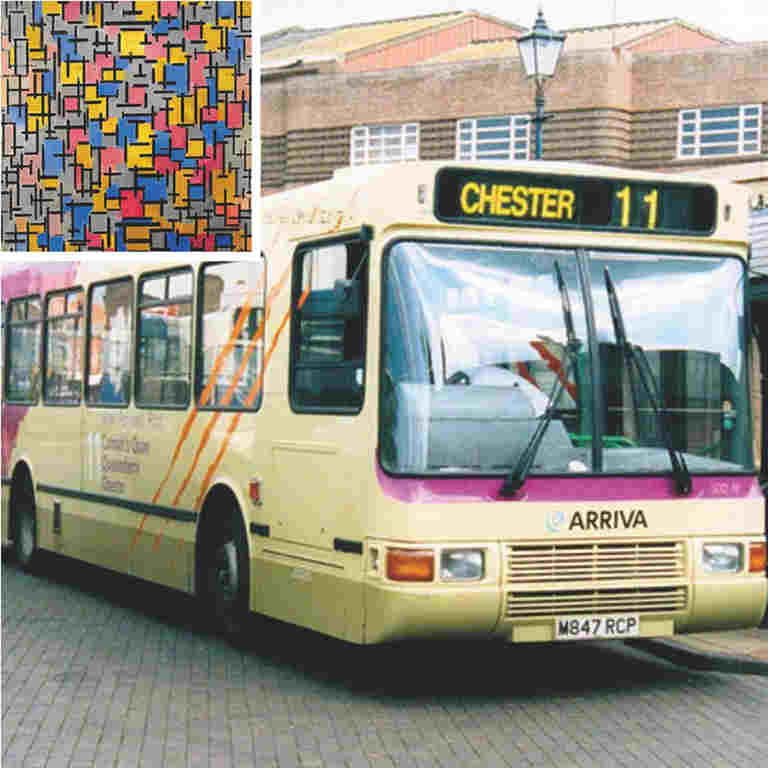
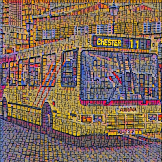
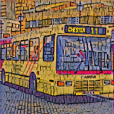
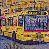
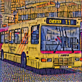
(a) Content&Style	(b) Stroke Size #1	(c) Stroke Size #2	(d) Stroke Size #3	(e) Mixed Strokes

Figure 1: Stylized results with different stroke sizes. All these results are produced by one single model in real-time using our proposed algorithm.

The current Fast Style Transfer approaches can be categorized into three classes, Per-Style-Per-Model (PSPM) [34, 35, 19, 24], Multiple-Style-Per-Model (MSPM) [39, 7, 26, 2], and Arbitrary-Style-Per-Model (ASPM) [18, 27]. The gist of PSPM is to train a feed-forward style-specific generator and to produce a corresponding stylized result with a forward pass. MSPM improves the efficiency by further incorporating multiple styles into one single generator. ASPM aims at transferring an arbitrary style through only one single model.

There is a trade-off between efficiency and quality for all such Fast Style Transfer algorithms [18, 27]. In terms of quality, PSPM is usually regarded to produce more appealing stylized results [35, 18]. However, PSPM is not flexible in terms of controlling perceptual factors (e.g., style-content tradeoff, color control, spatial control). Among these perceptual factors, strokes are one of the most important geometric primitives to characterize an artwork, as shown in Figure 1. In reality, for the same texture, different artists have their own way to place different sizes of strokes as a reflection of their unique “styles” (e.g., Monet and Pollock). To achieve different stroke sizes with PSPM, one possible solution is to train multiple models, which is time and space consuming. Another solution is to resize the input image to different scales, which will inevitably hurt the quality of stylization. None of these solutions, however, can achieve continuous stroke size control or produce distinct stroke sizes in different spatial regions without trading off quality and efficiency.

In this paper, we propose a stroke controllable Fast Style Transfer algorithm that can incorporate multiple stroke sizes into one single model and achieves flexible continuous stroke size control and spatial stroke size control. By analyzing the factors that influence the stroke size in stylized results, we propose to explicitly account for both the receptive field and the style image scale. To this end, we propose a StrokePyramid module to endow the network with adaptive receptive fields and different stroke sizes are learned with different receptive fields. We then introduce a progressive training strategy to make the network converge faster and an incremental training strategy to learn new stroke sizes upon a trained model. By combining two proposed runtime control techniques which are continuous stroke size control and spatial stroke size control, our network can produce distinct stroke sizes in different outputs or different spatial regions within the same output image.

In summary, our work has three primary contributions: 1) We analyze the factors that influence the stroke size in stylized results, and propose that both the receptive field and the style image scale should be considered for stroke size control in most cases. 2) We propose a stroke controllable style transfer network and two corresponding training strategies in order to achieve faster convergence and augment new stroke sizes upon a trained model respectively. 3) We present two runtime control strategies to empower our single model with the ability of producing continuous changes in stroke size and distinct stroke sizes in different spatial regions within the same output image. To the best of our knowledge, this is the first style transfer network that achieves continuous stroke size control and spatial stroke size control.

2 Related Work

We briefly review here perceptual factors in Fast Style Transfer as well as the involving regulating receptive field in neural networks.

Controlling perceptual factors in Fast Style Transfer. Stroke size control belongs to the domain of controlling perceptual factors during stylization. In this field, several significant works are recently presented. However, there are few efforts devoted to controlling stroke size during Fast Style Transfer. In [14], Gatys et al. study the color control and spatial control for Fast Style Transfer. Lu et al. further extend Gatys et al.’s work to meaningful spatial control by incorporating semantic content, achieving the so-called Fast Semantic Style Transfer [29]. Another related work is Wang et al.’s algorithm which aims to learn large brush strokes for high-resolution images [36]. They find that current Fast Style Transfer algorithms fail to paint large strokes in high-resolution images and propose a coarse-to-fine architecture to solve this problem. Note that the work in [36] is intrinsically different from this paper as one single pre-trained model in [36] still produces one stroke size for the same input image. A concurrent work in [39] also explores the issue of stroke size control. Compared with [39], our work has the benefits of flexible continuous and spatial stroke size control.

Regulating receptive field in neural networks. The receptive field is one of the basic concepts in convolutional neural networks, which refers to a region of the input image that one neuron is responsive to. It can affect the performance of the networks and becomes a critical issue in many tasks (e.g., semantic segmentation [40], image parsing). To regulate the receptive field, [38] proposes the operation of dilated convolution (also called atrous convolution in [4]), which supports the expansion of receptive field by setting different dilation values and is widely used in many generation tasks like [16, 10]. Another work in [5] further proposes a deformable convolution which augments the sampling locations in regular convolution with additional offsets. Furthermore, Wei et al. [37] propose a learning-based receptive field regulating method which is to inflate or shrink feature maps automatically.

3 Pre-analysis

We start by reviewing the concept of the stroke size. Consider an image in style transfer as a composition of a series of small stroke textons, which are referred as the fundamental geometric micro-structures in images [20, 41]. The stroke size of an image can be defined as the average scale of the composed stroke textons.

In the deep neural network based Fast Style Transfer, three factors are found to influence the stroke size, namely the scale of the style image [36], the receptive field in the loss network [14], and the receptive field in the generative network.

The objective style is usually learned by matching the style image’s gram-based statistics [13] in style transfer algorithms, which are computed over the feature maps from the pre-trained VGG network [32]. These gram-based statistics are scale-sensitive, i.e., they contain the scale information of the given style image. One reason for this characteristic is that the VGG features vary with the image scale. We also find that for other style statistics (e.g., BN-based statistics in [25]), it reaches the same conclusion. Therefore, given the same content image, generative networks trained with different scales of the style image can produce different stroke sizes.

Although the stroke in stylized results usually becomes larger with the increase of the style image scale, this is infeasible when the style image is scaled to a high resolution (e.g., $3000\times 3000$ pixels [14]). The reason for this problem is that a neuron in pre-trained VGG loss network can only affect a region with the receptive field size in the input image. When the stroke texton is much larger than the fixed receptive field in VGG loss network, there is no visual difference between a large and larger stroke texton in a relatively small region.

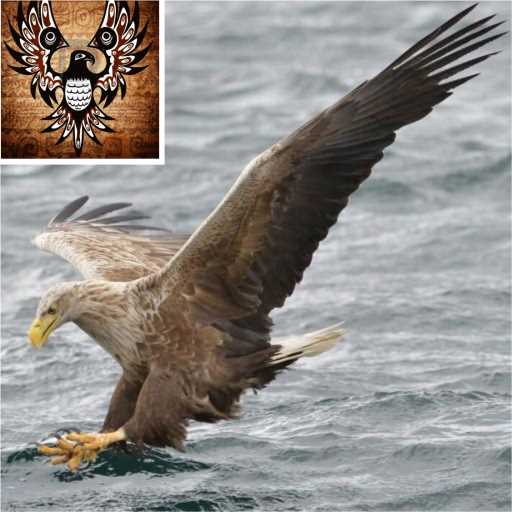
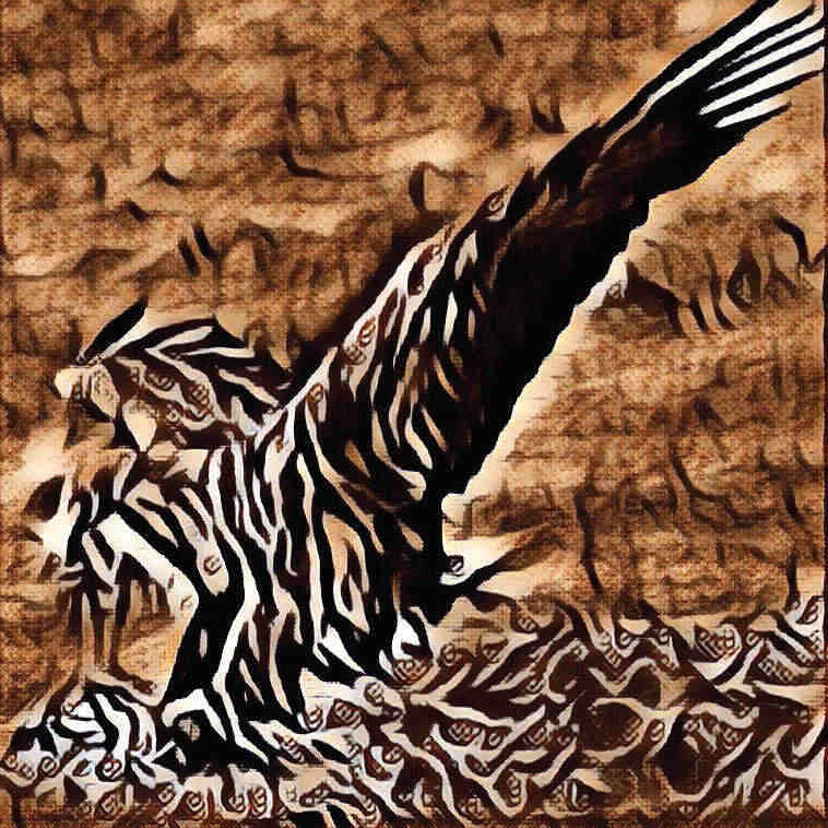
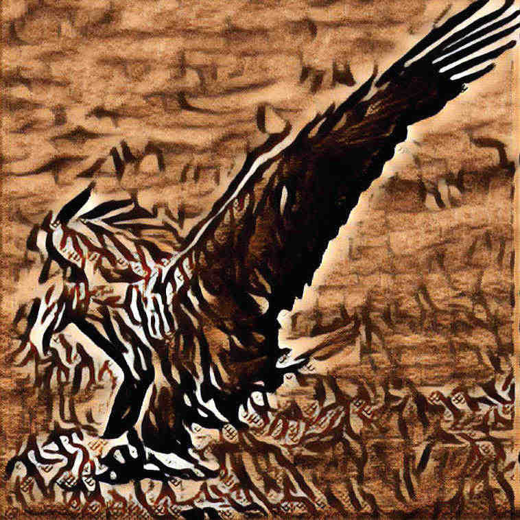
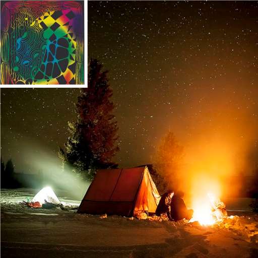
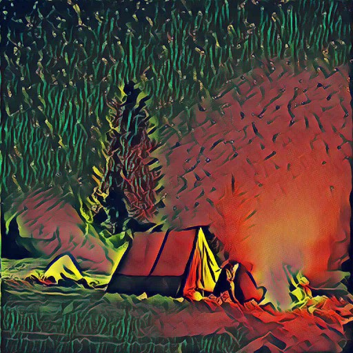
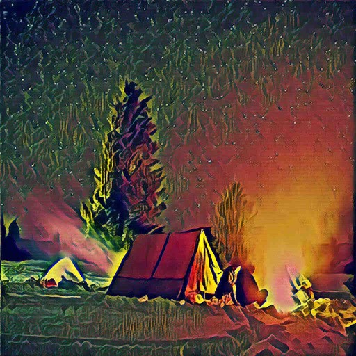
Content & Style	LRF Result	SRF Result	Content & Style	LRF Result	SRF Result

Figure 2: Results of learning the same size of large strokes with large and small receptive fields, respectively. LRF represents the result produced with a large receptive field and SRF represents the result produced with a small receptive field. Content images are credited to flickr users Kevin Robson and b togol.

Apart from these above two factors, we further find that the receptive field size in the generative network also has influence on the stroke size. In Figure 2, we change the receptive field size in the generative network and other factors remain the same. It is noticeable that a larger stroke size is produced with a larger receptive field for some styles. To explain this result, we interpret the training process of the generative network as teaching the convolutional kernels to paint a pre-defined size of stroke textons in each region with the size of receptive field. Therefore, given two different sizes of input images, the kernels of a trained network paint almost the same size of stroke textons in the same size of regions, as shown in Figure 3. In particular, when the receptive field in a generative network is smaller than the stroke texton, the kernels can only learn to paint a part of the whole stroke texton in each region, which influences the stroke size. Hence, for a large stroke size, the network needs larger receptive fields to learn the global stroke configuration. For a small stroke size, the network only needs to learn local features.

To sum up, both the scale of the style image and the receptive field in the generative network should generally be considered for stroke size control. As the style image is not high-resolution in most cases, the influence of the receptive field in the loss network is not considered in this work.

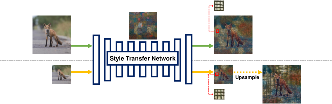
Figure 3: The feed-forward process of Fast Style Transfer. For the same size of regions in the outputs of both small and large input images respectively, their stroke sizes are almost the same. The content image is credited to flickr user BillChenSF.

4 Proposed Approach

4.1 Problem Formulation

Assume that $\mathcal{T}_{i}\in\mathbb{T}$ denotes the stroke size of an image, $\mathbb{T}$ denotes the set of all stroke sizes, and $I^{\mathcal{T}_{i}}$ represents an image $I$ with the stroke size $\mathcal{T}_{i}$. The problem studied in this paper is to incorporate different stroke sizes $\mathcal{T}_{i}\in\mathbb{T}$ into the feed-forward fast neural style transfer model. Firstly, we formulate the feed-forward stylization process as:

$$g(I_{c})=I_{o},\quad I_{o}\sim p(I_{o}|I_{c},I_{s}),$$ (1)

where $g$ is the trained generator. And the target statistic $p(I_{o})$ of the output image $I_{o}$ is characterized by two components, which are the semantic content statistics derived from the input image $I_{c}$, and the visual style statistics derived from the style image $I_{s}$.

Our feed-forward style transfer process for producing multiple stroke sizes can then be modeled as:

$$g^{\prime}(I_{c},\mathcal{T}_{i})=I^{\mathcal{T}_{i}}_{o},\quad I^{\mathcal{T}_{i}}_{o}\sim p(I^{\mathcal{T}_{i}}_{o}|I_{c},I_{s},\mathcal{T}_{i})\ (\mathcal{T}_{i}\in\mathbb{T}).$$ (2)

We aim to enable one single generator $g^{\prime}$ to produce stylized results with multiple stroke sizes $\mathcal{T}_{i}\in\mathbb{T}$ for the same content image $I_{c}$.

4.2 Network Architecture

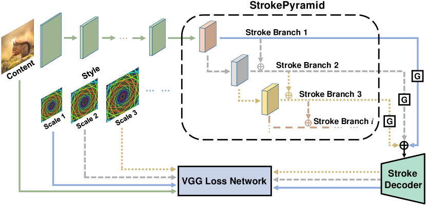
Figure 4: An overview of our network architecture with the StrokePyramid. It consists of several stroke branches with gating functions. Each stroke branch corresponds to a specific stroke size.

Based on the analysis in Section 3, to incorporate different stroke sizes into one single model, we propose to design a network with adaptive receptive fields and each receptive field is used to learn a corresponding size of stroke. The network architecture of our proposed approach is depicted in Figure 4.

Our network consists of three components. At the core of our network, a StrokePyramid module is proposed to decompose the network into several stroke branches. Each branch has a larger receptive field than the previous branch through progressively growing convolutional filters. In this way, our network also encourages stroke consistency (which refers to the consistency of stroke orientation, configuration, etc) between adjacent stroke size control results which should differ only in stroke sizes. By handling different stroke branches, the StrokePyramid can regulate the receptive field in the generative network. With different receptive fields, the network learns to paint strokes with different sizes. In particular, to better preserve the desired size of strokes, larger strokes are learned with larger receptive fields, as explained in Section 3. During the testing phase, given a signal which indicates the desired stroke size, the StrokePyramid automatically adapts the receptive field in the network and the stylized result with a corresponding stroke size can be produced.

In addition to the StrokePyramid, there are two more components in the network, namely the pre-encoder and the stroke decoder. The pre-encoder module refers to the first few layers in the network and is shared among different stroke branches to learn both the semantic content of a content image and the basic appearances of a style. The stroke decoder module takes the feature maps from the StrokePyramid as input and decodes the stroke feature into the stylized result with a corresponding stroke size. To determine which stroke feature to decode, we augment a gating function $G$ in each stroke branch. The gating function $G$ is defined as

$$G(\mathcal{F}^{\mathcal{B}_{s_{i}}})=a_{i}\mathcal{F}^{\mathcal{B}_{s_{i}}},\quad\sum\limits_{i}{a_{i}}=1\ (0\leq a_{i}\leq 1),$$ (3)

where $\mathcal{F}^{\mathcal{B}_{s_{i}}}$ is the output feature map of the branch $\mathcal{B}_{s_{i}}$ in the StrokePyramid, which corresponds to the stroke size $\mathcal{T}_{i}$. For the selection of $a$, at the training stage, $a_{i}$ is binary. More specifically, $a_{i}=1$ when $i=k$ (i.e., the selected stroke branch to be trained is $\mathcal{B}_{s_{k}}$). Otherwise, $a_{i}=0$ when $i\neq k$. At the testing stage, $a_{i}$ can be fractional, which is the basis of our continuous stroke size control.

All the stroke features from the StrokePyramid need to go through the gating function and then be fed into the stroke decoder $Dec$ to be decoded into the output result $I^{\mathcal{T}_{k}}_{o}$ with the desired stroke size:

$$Dec(\sum\limits_{i}{G(\mathcal{F}^{\mathcal{B}_{s_{i}}})})=I^{\mathcal{T}_{k}}_{o}.$$ (4)

4.3 Loss Function

Semantic loss. The semantic loss is defined to preserve the semantic information in the content image, which is formulated as the Euclidean distance between the content image $I_{c}$ and the output stylized image $I_{o}$ in the feature space of the VGG network [13].

Assume that $\mathcal{F}^{l}(I)\in\mathbb{R}^{C\times H\times W}$ represents the feature map at layer $l$ in VGG network with a given image $I$, where $C$, $H$ and $W$ denote the number of channels, the height and width of the feature map respectively. The semantic content loss is then defined as:

$$\mathcal{L}_{c}=\sum\mathop{}_{l\in\{l_{c}\}}\lVert\mathcal{F}^{l}(I_{c})-\mathcal{F}^{l}(I_{o})\rVert^{2},$$ (5)

where $\{l_{c}\}$ represents the set of VGG layers used to compute the content loss.

Stroke loss. The visual style statistics can be well represented by the correlations between filter responses of the style image $I_{s}$ in different layers of pre-trained VGG network. These feature correlations can be obtained by computing the Gram matrix over the feature map at a certain layer in VGG network. As the gram-based statistic is scale-sensitive, representations of different stroke sizes can be obtained by simply resizing the given style image.

By reshaping $\mathcal{F}^{l}(I)$ into $\mathcal{F}^{l}(I)^{\prime}\in\mathbb{R}^{C\times(H\times W)}$, the Gram matrix $\mathcal{G}(\mathcal{F}^{l}(I)^{\prime})\in\mathbb{R}^{C\times C}$ over feature map $\mathcal{F}^{l}(I)^{\prime}$ can be computed as:

$$\mathcal{G}(\mathcal{F}^{l}(I_{s})^{\prime})=[\mathcal{F}^{l}(I_{s})^{\prime}][\mathcal{F}^{l}(I_{s})^{\prime}]^{T}.$$ (6)

The stroke loss for size $\mathcal{T}_{k}$ can be therefore defined as:

$$\mathcal{L}_{\mathcal{T}_{k}}=\sum\mathop{}_{l\in\{l_{s}\}}\lVert\mathcal{G}(\mathcal{F}^{l}(\mathcal{R}(I_{s},\mathcal{T}_{k}))^{\prime})-\mathcal{G}(\mathcal{F}^{l}(I_{o}^{\mathcal{B}_{s_{k}}})^{\prime})\rVert^{2},$$ (7)

where $\mathcal{R}$ represents the function that resizes the style image to an appropriate scale according to the desired stroke size $\mathcal{T}_{k}$, and $I_{o}^{\mathcal{B}_{s_{k}}}$ represents the output of the $k$-th stroke branch. $\{l_{s}\}$ is the set of VGG layers used for style loss.

The total loss for stroke branch $\mathcal{B}_{s_{k}}$ is then written as:

$$\mathcal{L}_{\mathcal{B}_{s_{k}}}=\alpha\mathcal{L}_{c}+\beta_{k}\mathcal{L}_{\mathcal{T}_{k}}+\gamma\mathcal{L}_{tv},$$ (8)

where $\alpha$, $\beta$ and $\gamma$ are balancing factors. $\mathcal{L}_{tv}$ is a total variation regularization loss to encourage smoothness in the generated images.

4.4 Training Strategies

Progressive training. To train different stroke branches in one single network, we propose a progressive training strategy. This training strategy stems from the intuition that the training of the latter stroke branch benefits from the knowledge of the previously learned branches. Taken this into consideration, the network learns different stroke sizes with different stroke branches progressively. Assume that the number of the stroke sizes to be learned is $K$. For every $K$ iterations, the network firstly updates the first stroke branch in order to learn the smallest size of stroke. Then, based on the learned knowledge of the first branch, the network uses the second stroke branch to learn the second stroke size with a corresponding scale of the style image. In particular, since the second stroke branch grows the convolutional filters on the basis of the first stroke branch, the updated components in the previous iteration are also adjusted. Similarly, the following stroke branches are updated with the same progressive process. In the next $K$ iterations, the network repeats the above progressive process, since we need to ensure that the network preserves the previously learned stroke sizes.

Incremental training. We also propose a flexible incremental training strategy to efficiently augment new stroke sizes upon a trained model. Given a new desired stroke size, instead of learning from scratch, our algorithm incrementally learns the new stroke size by adding one single layer as a new stroke branch in the StrokePyramid. The position of the augmented layer depends on the previously learned stroke sizes and their corresponding receptive fields. By fixing other network components and only updating the augmented layer, the network learns to paint a new size of strokes on the basis of the previously learned stroke features and thus can reach convergence quickly.

4.5 Runtime Control Strategies

Continuous stroke size control. One of the advantages of our algorithm over previous approaches is that our algorithm can endow one single model with the ability of finer continuous stroke size control. We propose a stroke interpolation strategy to exploit our architecture to interpolate between trained stroke sizes in the feature embedding space, instead of training with tons of style image scales.

Given a content image $I_{c}$, we assume that $\mathcal{F}^{\mathcal{B}_{s_{m}}}$ and $\mathcal{F}^{\mathcal{B}_{s_{n}}}$ are two output feature maps in the StrokePyramid, which can be decoded into the stylized results with two stroke sizes $I^{\mathcal{T}_{m}}_{o}$ and $I^{\mathcal{T}_{n}}_{o}$ respectively. The interpolated feature $\mathcal{F}^{\mathcal{B}_{\widetilde{s}}}$ can then be obtained by controlling the gating functions in Figure 4 to interpolate between output feature maps in the StrokePyramid:

$$\mathcal{F}^{\mathcal{B}_{\widetilde{s}}}=a_{m}\mathcal{F}^{\mathcal{B}_{s_{m}}}+(1-a_{m})\mathcal{F}^{\mathcal{B}_{s_{n}}}.$$ (9)

By gradually changing the value of $a_{m}$ and feeding the obtained $\mathcal{F}^{\mathcal{B}_{\widetilde{s}}}$ into the stroke decoder module, stylized results with arbitrary intermediate stroke sizes $I^{\mathcal{\widetilde{T}}}_{o}$ can be produced.

To our knowledge, none of previous approaches considers this much finer continuous stroke size control. However, from our point of view, there may be some possible solutions which can be derived from current approaches: 1) Directly interpolate between stylized results with different stroke sizes in the pixel space. 2) Design a network with different encoders but a shared decoder, and train each encoder and shared decoder jointly with different style image scales. Then interpolate between two representations from the encoders. 3) Rescale the style image and use ASPM methods to produce the corresponding results.

However, our algorithm outperforms these solutions in the following aspects correspondingly: 1) We manipulate the interpolation in the feature embedding space to achieve perceptually superior results [19, 6]. 2) Our stroke representations are obtained with different receptive fields in the StrokePyramid. As explained and verified in Section 3 and Figure 2, our stroke representations are perceptually better than those obtained with the same receptive field. In addition, the results of our proposed StrokePyramid are more consistent in stroke orientations and configurations during stroke size control. The comparison results can be found in the supplementary material. 3) ASPM compromises on visual quality and is generally not effective at producing fine strokes and details. Our algorithm outperforms ASPM in terms of quality and also stylization speed.

Spatial stroke size control. Previously, in the community of Fast Style Transfer, stylized results usually have almost the same stroke size across the whole image, which is impractical in the real case. Our algorithm supports mixed stroke sizes in different spatial regions and also with only one single model. In this way, the contrast information in stylized results can be enhanced.

Our spatial stroke size control is achieved by feeding masked content image through different corresponding stroke branches by controlling the gating functions, and then combining these stylized results. The mask can be obtained either by manual labelling or forwarding the content image through a pre-trained semantic segmentation network, e.g., DeepLabv2 [4]. By further combining our continuous stroke size control strategy, our algorithm provides practitioners a much finer control over the stylized results.

5 Experiment

5.1 Implementation Details

Our proposed network is trained on MS-COCO dataset [28]. All the images are cropped and resized to $512\times 512$ pixels before training. We adopt the Adam optimizer [22] during training. The pre-trained VGG-19 network [32] is selected as the loss network and $\{relu1\_1,relu2\_1,relu3\_1,relu4\_1,relu5\_1\}$ are used as the style layers and $relu4\_2$ is used as the content layer. By default, the number of initially learned stroke sizes is set to 3 to ensure the ability of stroke decoder, and the scales are 256, 512, and 768 for different stroke sizes for all styles in our experiment. More information can be found in the supplementary material.

	(a) Content & Style

& (b) Training a separate generator(c) Image resizing + forwarding + SR (d) Our proposed approach

Figure 5: Quality comparison of our proposed algorithm and aforementioned two possible stroke control solutions in Section 4. SR represents the image super-resolution technique [21]. The images in the second line represent the zoom regions in the red frames.

5.2 Qualitative Evaluation

Comparison with previous solutions. Sample results of our algorithm and two aforementioned possible solutions are shown in Figure 5.1 (Figure 5.1(b) is produced by [19]). Our algorithm achieves comparable results with the first possible solution in Figure 5.1(b) regarding quality while preserving the flexibility of the second possible solution in Figure 5.1(c). Figure 6 shows sample results of our algorithm and other Fast Style Transfer algorithms. Compared with [19, 35], our results with different stroke sizes are more consistent in stroke orientations and stroke configurations (the positions of the blue strokes in Figure 6). The stroke orientations and configurations in [19, 35]’s results are more random, since they use different encoder-decoder pairs to learn different stroke sizes separately. By contrast, our StrokePyramid can encourage stroke consistency between adjacent stroke size control results which should differ only in stroke sizes. Compared with [36], our algorithm can exploit one single trained model to achieve continuous and spatial stroke size control. Also, our model size is much smaller than [36], which is 0.99 MB vs 32.2 MB. Compared with other single-model stroke size control algorithms [18, 27], our results capture finer strokes and more details. Also, our results seem to be superior in terms of visual quality. More explanations and comparison results can be found in the supplementary material.

Runtime user controls. In Figure 7, we show sample results of our proposed continuous stroke size control strategy. Our network is trained with three scales of the style image as default and we do the stroke interpolation between them to obtain totally six stroke sizes. The test content image is never seen during training. We also demonstrate the results of [18, 27] for comparison, as explained in Section 4.5. We compare the results of different algorithms both globally and locally. Globally, our algorithm seems to achieve superior performance in terms of visual quality. Locally, compared with [18, 27], our algorithm is more effective at producing fine strokes and preserving details. In addition, as shown in Figure 8, the absolute differences of our adjacent continuous stroke size control results have a much clearer stroke contour, which indicates that most strokes in our results increase or decrease in size together during continuous stroke size control. We have also produced a sample video to demonstrate our continuous stroke size control in the supplementary material. Figure 5.1 demonstrates the results of our spatial stroke size control strategy. Our spatial stroke size control is realized with only one single model. Compared with Figure 5.1(c), controlling the stroke size in different spatial regions can enhance the contrast of stylized images and make AI-Created Art much closer to Human-Created Art.

Multiple Models

Single Model

	[19]	[35]	[36]			[18]	[27]	Ours
SS #1:
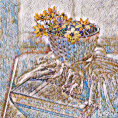
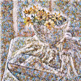
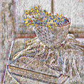
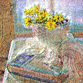
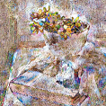
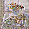
SS #2:
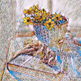
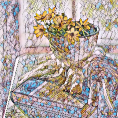
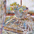
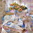
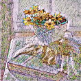
SS #3:

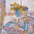
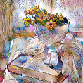
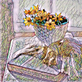
Figure 6: Some example results of different stroke sizes (SS) produced by our algorithm and other Fast Style Transfer algorithms. Each column represents the results of the same algorithm. The style image is the same with Figure 5.1.

[18]:

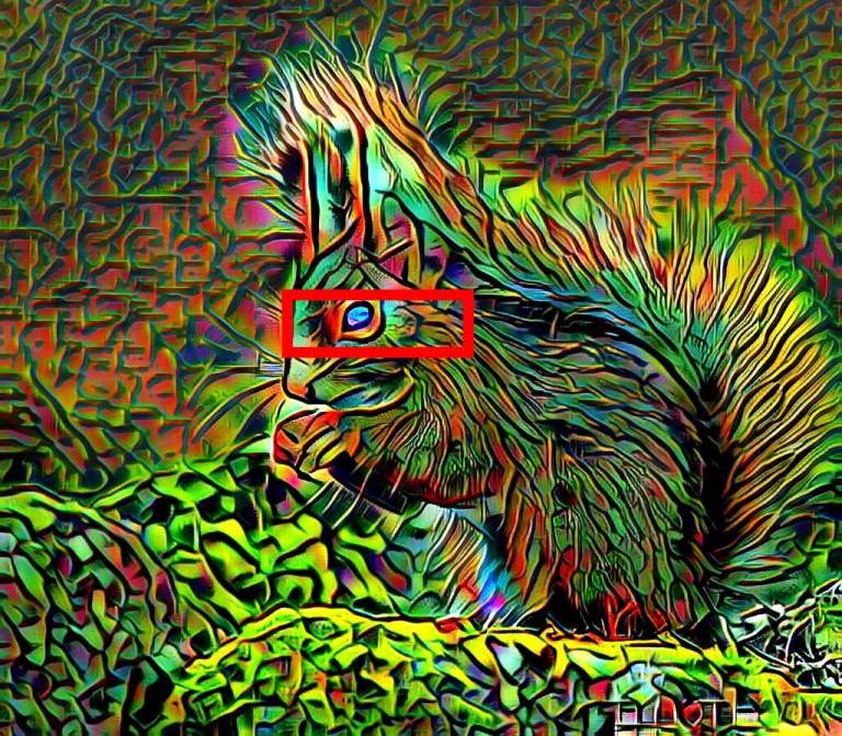
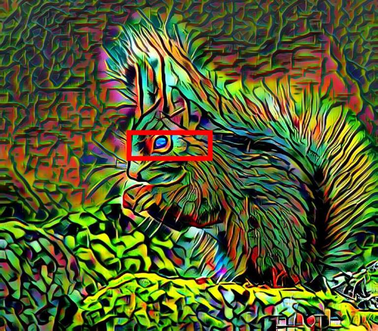
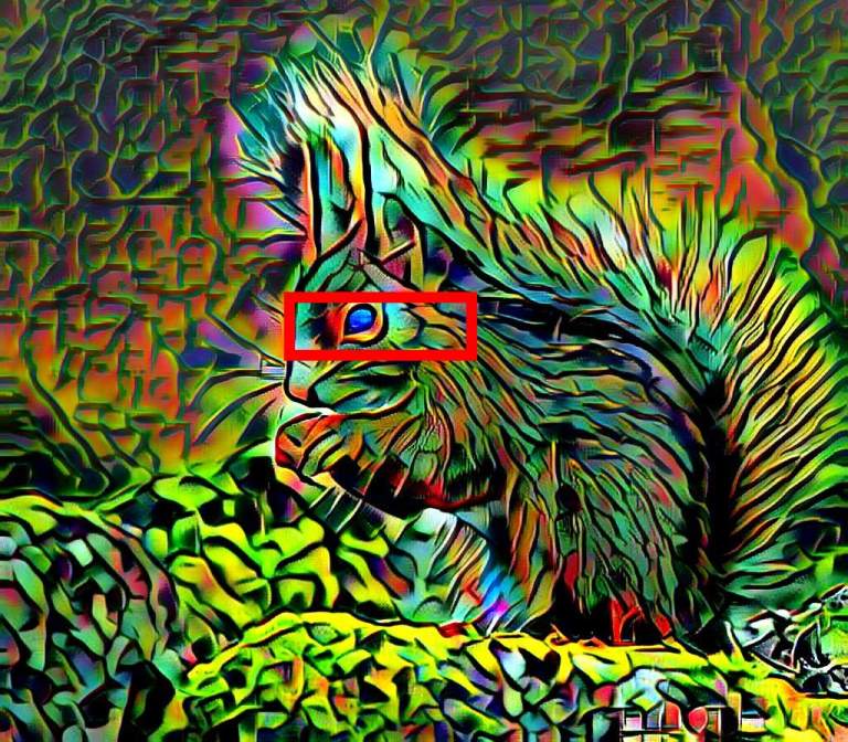
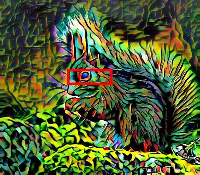
[27]:

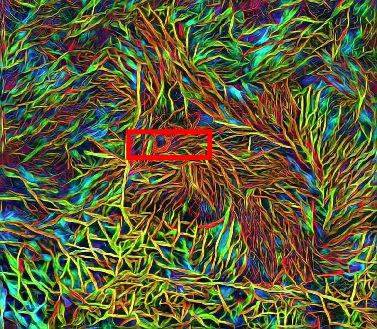
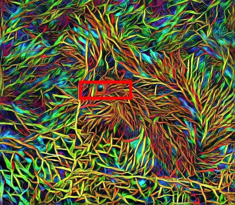
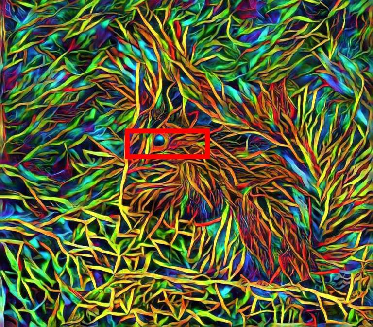
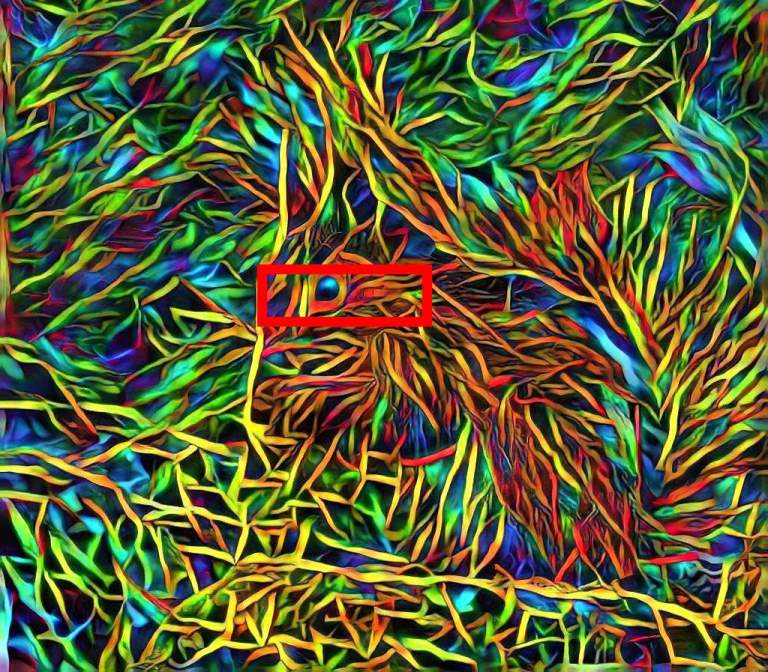
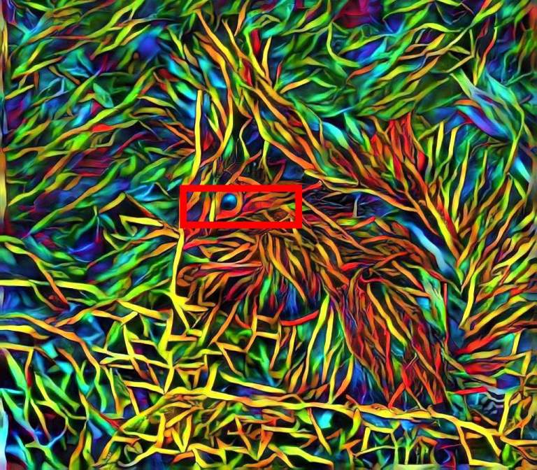
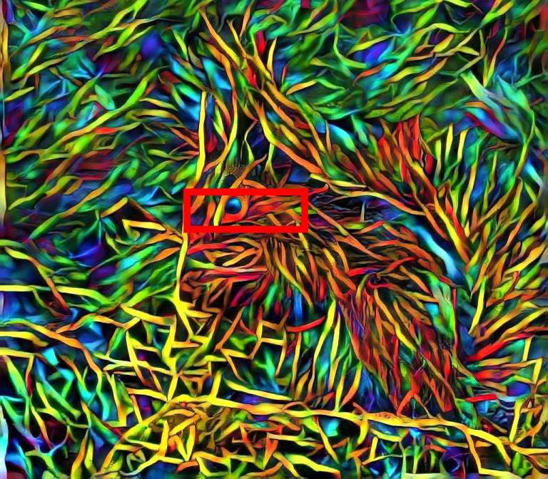
Ours:

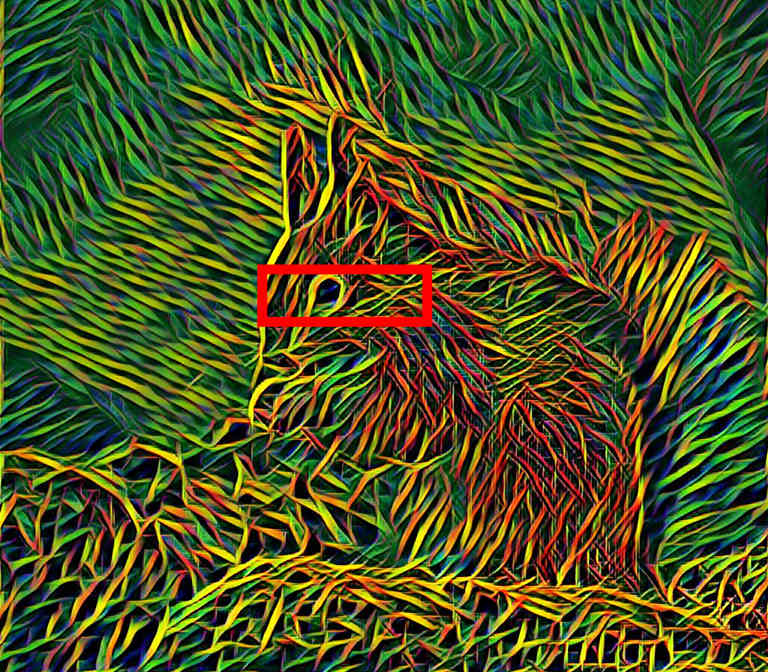
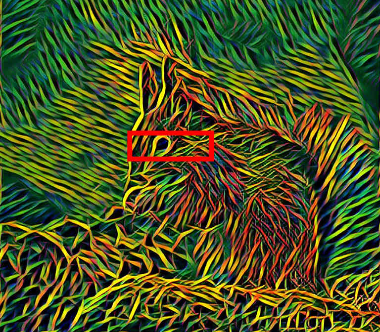
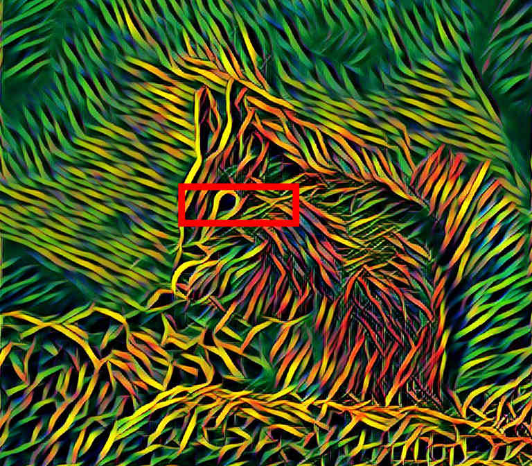
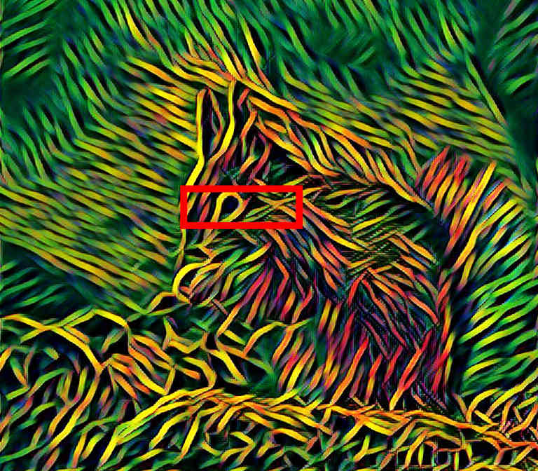
Figure 7: Results of continuous stroke size control. We zoom in on the same region (red frame) to observe the variations of stroke sizes. Our algorithm produces finer strokes and details. The content and style image can be found in Figure 4.

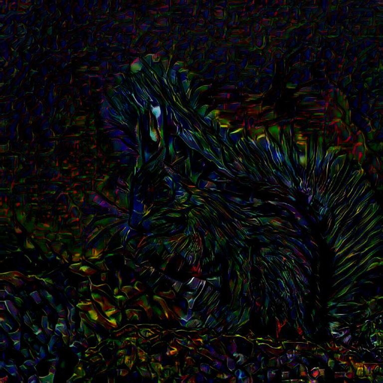
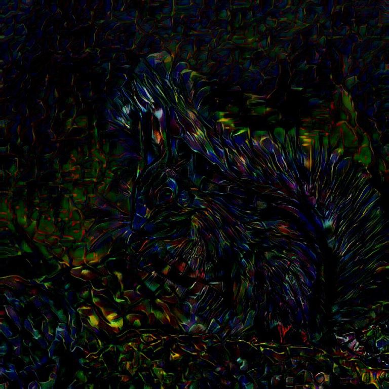
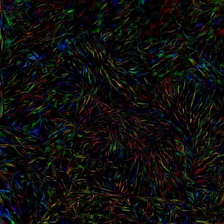
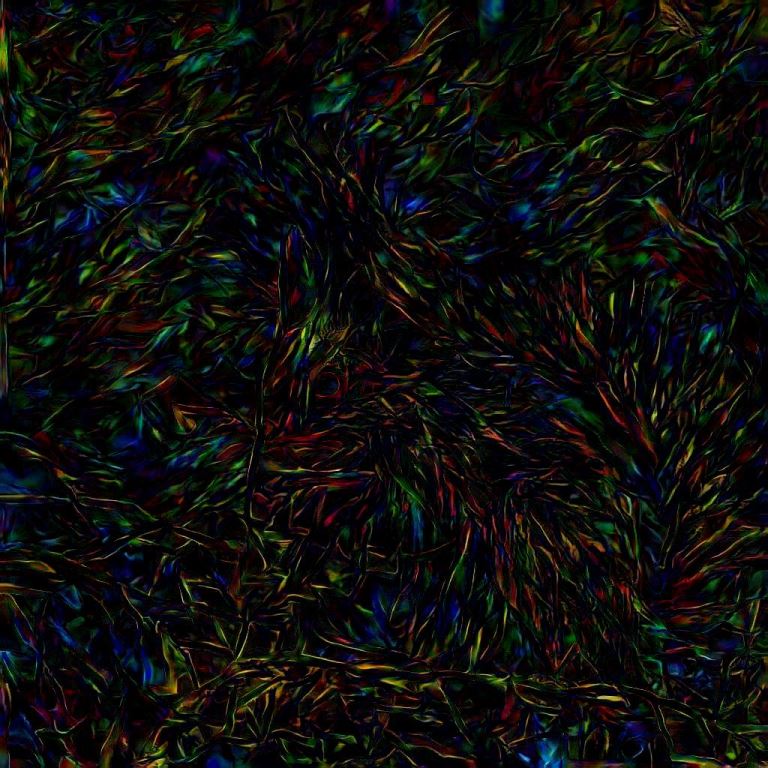
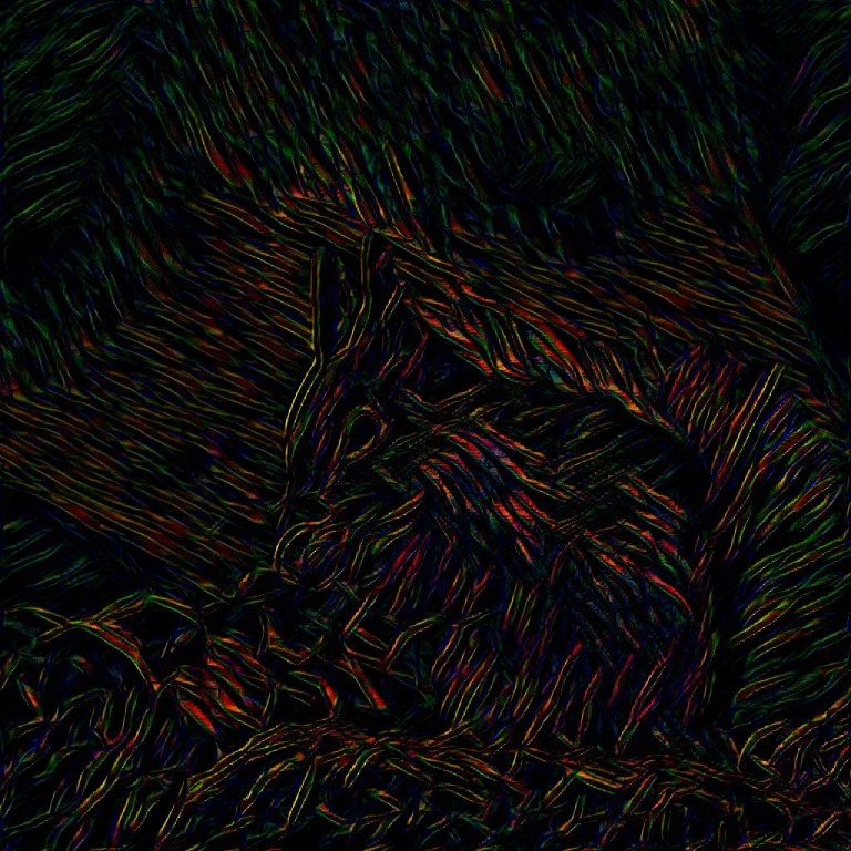
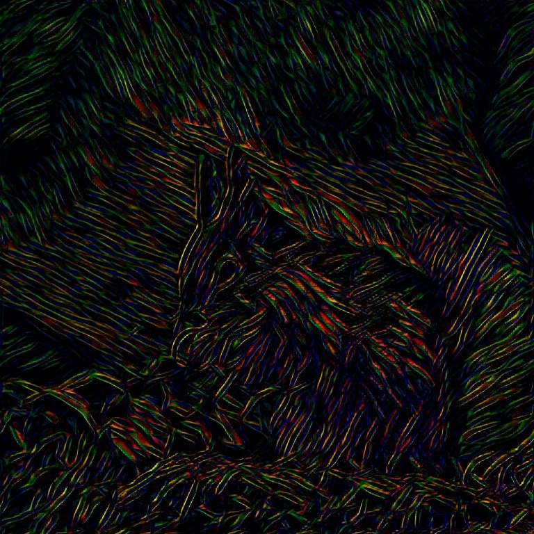
[18]’s differential images		[27]’s differential images		Our differential images

Figure 8: Results of the absolute differences of adjacent images in each row of Figure 7.

& (b) Content mask (c) Same stroke size across image (d) Our spatial stroke size control

Figure 9: Our algorithm allows flexible spatial stroke size control during stylization. The result produced by our single model can have mixed stroke sizes, which is more consistent with an artist’s artwork in reality.

5.3 Quantitative Evaluation

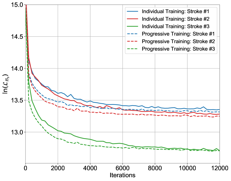
(a) Progressive training.

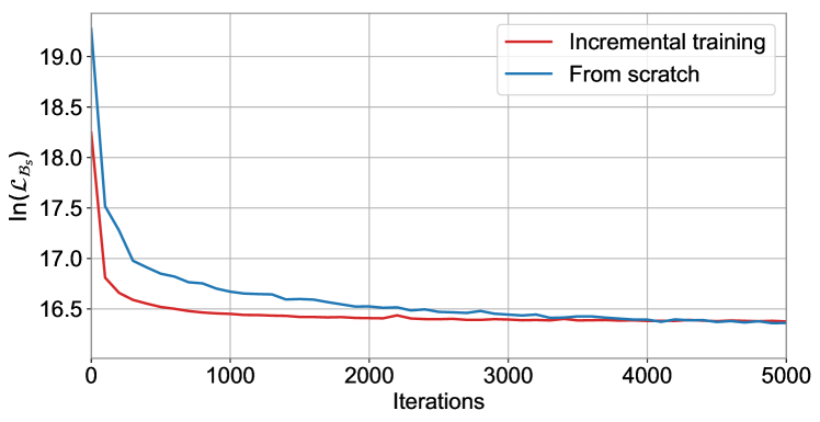
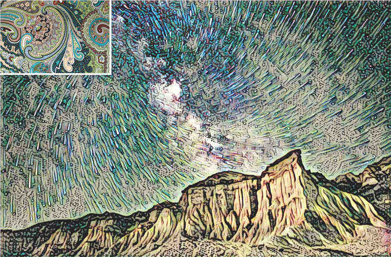
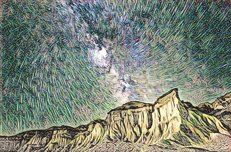
(b) Incremental training.

Figure 10: Training curve comparisons of the training strategies. The bottom left and right images in (b) are the results of incremental training and training from scratch.

For the quantitative evaluation, we focus on three evaluation metrics, which are: training curves during progressive training and incremental training; average content and style loss for test content images; training time for our single model and corresponding generating time for results with different stroke sizes.

Training curve analysis. To demonstrate the effectiveness of our progressive training strategy, we record the stroke losses when learning several sizes of strokes progressively and learning different strokes individually. The result is shown in Figure 10(a). The reported loss values were averaged over 15 randomly selected batches of content images. It can be observed that the network which progressively learns multiple stroke sizes converges relatively faster than the one which learns only one single stroke size individually. The result indicates that during progressive training, the latter stroke branch benefits from the learned knowledge of the previous branches, and can even improve the training of previous branches through a shared network component in turn. To validate our stroke incremental training strategy, we present both the training curves of the incremental training and training from scratch in Figure 10(b). While achieving comparable stylization quality, incrementally learning a stroke can significantly speed up the training process compared to learning from scratch.

Average loss analysis. To measure how well the loss function is minimized, we compare the average content and style loss of our algorithm with other style transfer methods. The recorded values are averaged over 100 content images and 5 style images. For each style, we calculate the average loss of the three stroke sizes. As shown in Figure 11, the average style loss of our algorithm is similar to [35], and our average content loss is slightly lower than [35]. This indicates that our algorithm achieves comparable or slightly better performance than [35] regarding the ability to minimize the loss function.

Speed and model size analysis. Fully training one single model with three stroke sizes takes about 2 hours on a single NVIDIA Quadro M6000. For generating time, it takes averagely 0.09 seconds to stylize an image with size $1024\times 1024$ on the same GPU using our algorithm. Since our network architecture is similar with [19, 35] but with a shorter path for some stroke sizes, our algorithm can be on average faster than [19, 35], and further faster than Wang et al.’s algorithm, Huang and Belongie’s algorithm and Li et al.’s algorithm according to the speed analysis in [36, 18, 27]. The size of our model on disk is 0.99 MB.

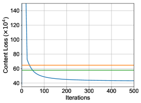
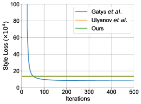
(a) Content loss	(b) Style loss

Figure 11: Comparisons of the average content and style loss of our algorithm with state-of-the-art Neural Style Transfer algorithms.

6 Discussion and Conclusion

In this paper, we introduce a fine and flexible stroke size control approach for Fast Style Transfer. Without trading off quality and efficiency, our algorithm is the first to achieve continuous and spatial stroke size control with one single model. Our idea can also be directly applied to MSPM methods. For the application in the real world, our work provides a new tool for practitioners to inject their own artistic preferences into style transfer results, which can be directly applied in the production software and entertainment. Regarding the significance of our work for the larger vision community beyond style transfer, our work takes one step in the direction of learning adaptive receptive fields in the human vision system and primarily validates its significance in style transfer. In the future, we hope to further explore the use of learning adaptive receptive fields to benefit the larger vision community, e.g., multi-scale deep image aesthetic assessment, deep image compression, deep image colorization, etc.

Our work is only the first step towards the finer and more flexible stroke size control, and there are still some issues remaining to be addressed. The most interesting one is probably the automatic spatial stroke size control in one shot. The process of spatial stroke size control will be more efficient and user-friendly if the semantic segmentation network can be incorporated as a module in our network, so as to support the automatic determination of the stroke sizes for different spatial regions. Besides, the relations among the style representations of different scales of the same style image still remains unclear. The transformation from the style representation of one scale to that of another is the key to a more flexible stroke size control. Acknowledgments. The first two authors contributed equally. Mingli Song is the corresponding author. This work is supported by National Key Research and Development Program (2016YFB1200203), National Natural Science Foundation of China (61572428, U1509206), Fundamental Research Funds for the Central Universities (2017FZA5014) and Key Research, Development Program of Zhejiang Province (2018C01004) and ARC FL-170100117, DP-180103424 of Australia.

References

- [1] Chen, D., Liao, J., Yuan, L., Yu, N., Hua, G.: Coherent online video style transfer. Proceedings of the IEEE International Conference on Computer Vision (2017)
- [2] Chen, D., Yuan, L., Liao, J., Yu, N., Hua, G.: Stylebank: An explicit representation for neural image style transfer. In: Proceedings of the IEEE Conference on Computer Vision and Pattern Recognition (2017)
- [3] Chen, D., Yuan, L., Liao, J., Yu, N., Hua, G.: Stereoscopic neural style transfer. Proceedings of the IEEE Conference on Computer Vision and Pattern Recognition (2018)
- [4] Chen, L.C., Papandreou, G., Kokkinos, I., Murphy, K., Yuille, A.L.: Deeplab: Semantic image segmentation with deep convolutional nets, atrous convolution, and fully connected crfs. IEEE Transactions on Pattern Analysis and Machine Intelligence (2017)
- [5] Dai, J., Qi, H., Xiong, Y., Li, Y., Zhang, G., Hu, H., Wei, Y.: Deformable convolutional networks. In: Proceedings of the IEEE International Conference on Computer Vision (2017)
- [6] Dosovitskiy, A., Brox, T.: Generating images with perceptual similarity metrics based on deep networks. In: Advances in Neural Information Processing Systems. pp. 658–666 (2016)
- [7] Dumoulin, V., Shlens, J., Kudlur, M.: A learned representation for artistic style. In: International Conference on Learning Representations (2017)
- [8] Efros, A.A., Freeman, W.T.: Image quilting for texture synthesis and transfer. In: Proceedings of the 28th annual conference on Computer graphics and interactive techniques. pp. 341–346. ACM (2001)
- [9] Elad, M., Milanfar, P.: Style transfer via texture synthesis. IEEE Transactions on Image Processing 26(5), 2338–2351 (2017)
- [10] Fan, Q., Chen, D., Yuan, L., Hua, G., Yu, N., Chen, B.: Decouple learning for parameterized image operators. In: European Conference on Computer Vision (2018)
- [11] Frigo, O., Sabater, N., Delon, J., Hellier, P.: Split and match: Example-based adaptive patch sampling for unsupervised style transfer. In: Proceedings of the IEEE Conference on Computer Vision and Pattern Recognition. pp. 553–561 (2016)
- [12] Gatys, L.A., Ecker, A.S., Bethge, M.: Texture synthesis using convolutional neural networks. In: Advances in Neural Information Processing Systems. pp. 262–270 (2015)
- [13] Gatys, L.A., Ecker, A.S., Bethge, M.: Image style transfer using convolutional neural networks. In: Proceedings of the IEEE Conference on Computer Vision and Pattern Recognition. pp. 2414–2423 (2016)
- [14] Gatys, L.A., Ecker, A.S., Bethge, M., Hertzmann, A., Shechtman, E.: Controlling perceptual factors in neural style transfer. In: Proceedings of the IEEE Conference on Computer Vision and Pattern Recognition (2017)
- [15] Gooch, B., Gooch, A.: Non-photorealistic rendering. A. K. Peters, Ltd., Natick, MA, USA (2001)
- [16] He, M., Chen, D., Liao, J., Sander, P.V., Yuan, L.: Deep exemplar-based colorization. ACM Transactions on Graphics (Proc. of Siggraph 2018) (2018)
- [17] Hertzmann, A., Jacobs, C.E., Oliver, N., Curless, B., Salesin, D.H.: Image analogies. In: Proceedings of the 28th annual conference on Computer graphics and interactive techniques. pp. 327–340. ACM (2001)
- [18] Huang, X., Belongie, S.: Arbitrary style transfer in real-time with adaptive instance normalization. In: Proceedings of the IEEE International Conference on Computer Vision (2017)
- [19] Johnson, J., Alahi, A., Fei-Fei, L.: Perceptual losses for real-time style transfer and super-resolution. In: European Conference on Computer Vision. pp. 694–711 (2016)
- [20] Julesz, B., et al.: Textons, the elements of texture perception, and their interactions. Nature 290(5802), 91–97 (1981)
- [21] Kim, J., Kwon Lee, J., Mu Lee, K.: Accurate image super-resolution using very deep convolutional networks. In: Proceedings of the IEEE Conference on Computer Vision and Pattern Recognition. pp. 1646–1654 (2016)
- [22] Kingma, D., Ba, J.: Adam: A method for stochastic optimization. In: International Conference on Learning Representations (2015)
- [23] Li, C., Wand, M.: Combining markov random fields and convolutional neural networks for image synthesis. In: Proceedings of the IEEE Conference on Computer Vision and Pattern Recognition. pp. 2479–2486 (2016)
- [24] Li, C., Wand, M.: Precomputed real-time texture synthesis with markovian generative adversarial networks. In: European Conference on Computer Vision. pp. 702–716 (2016)
- [25] Li, Y., Wang, N., Liu, J., Hou, X.: Demystifying neural style transfer. In: Proceedings of the Twenty-Sixth International Joint Conference on Artificial Intelligence, IJCAI-17. pp. 2230–2236 (2017). https://doi.org/10.24963/ijcai.2017/310, https://doi.org/10.24963/ijcai.2017/310
- [26] Li, Y., Chen, F., Yang, J., Wang, Z., Lu, X., Yang, M.H.: Diversified texture synthesis with feed-forward networks. In: Proceedings of the IEEE Conference on Computer Vision and Pattern Recognition (2017)
- [27] Li, Y., Fang, C., Yang, J., Wang, Z., Lu, X., Yang, M.H.: Universal style transfer via feature transforms. In: Advances in Neural Information Processing Systems (2017)
- [28] Lin, T.Y., Maire, M., Belongie, S., Hays, J., Perona, P., Ramanan, D., Dollár, P., Zitnick, C.L.: Microsoft coco: Common objects in context. In: European conference on computer vision. pp. 740–755. Springer (2014)
- [29] Lu, M., Zhao, H., Yao, A., Xu, F., Chen, Y., Zhang, L.: Decoder network over lightweight reconstructed feature for fast semantic style transfer. In: Proceedings of the IEEE International Conference on Computer Vision (2017)
- [30] Prisma Labs, I.: Prisma: Turn memories into art using artificial intelligence (2016), http://prisma-ai.com
- [31] Rosin, P., Collomosse, J.: Image and video-based artistic stylisation, vol. 42. Springer Science & Business Media (2012)
- [32] Simonyan, K., Zisserman, A.: Very deep convolutional networks for large-scale image recognition. arXiv preprint arXiv:1409.1556 (2014)
- [33] Strothotte, T., Schlechtweg, S.: Non-photorealistic computer graphics: modeling, rendering, and animation. Morgan Kaufmann (2002)
- [34] Ulyanov, D., Lebedev, V., Vedaldi, A., Lempitsky, V.: Texture networks: Feed-forward synthesis of textures and stylized images. In: International Conference on Machine Learning. pp. 1349–1357 (2016)
- [35] Ulyanov, D., Vedaldi, A., Lempitsky, V.: Improved texture networks: Maximizing quality and diversity in feed-forward stylization and texture synthesis. In: Proceedings of the IEEE Conference on Computer Vision and Pattern Recognition (2017)
- [36] Wang, X., Oxholm, G., Zhang, D., Wang, Y.F.: Multimodal transfer: A hierarchical deep convolutional neural network for fast artistic style transfer. In: Proceedings of the IEEE Conference on Computer Vision and Pattern Recognition (2017)
- [37] Wei, Z., Sun, Y., Wang, J., Lai, H., Liu, S.: Learning adaptive receptive fields for deep image parsing network. In: Proceedings of the IEEE Conference on Computer Vision and Pattern Recognition. pp. 2434–2442 (2017)
- [38] Yu, F., Koltun, V.: Multi-scale context aggregation by dilated convolutions. In: International Conference on Learning Representations (2016)
- [39] Zhang, H., Dana, K.: Multi-style generative network for real-time transfer. arXiv preprint arXiv:1703.06953 (2017)
- [40] Zhang, H., Dana, K., Shi, J., Zhang, Z., Wang, X., Tyagi, A., Agrawal, A.: Context encoding for semantic segmentation. In: Proceedings of the IEEE Conference on Computer Vision and Pattern Recognition (2018)
- [41] Zhu, S.C., Guo, C.E., Wang, Y., Xu, Z.: What are textons? International Journal of Computer Vision 62(1), 121–143 (2005)