Transient shear banding in the nematic dumbbell model of liquid crystalline polymers

Abstract

In the shear flow of liquid crystalline polymers (LCPs) the nematic director orientation can align with the flow direction for some materials, but continuously tumble in others. The nematic dumbbell (ND) model was originally developed to describe the rheology of flow-aligning semi-flexible LCPs, and flow-aligning LCPs are the focus in this paper. In the shear flow of monodomain LCPs it is usually assumed that the spatial distribution of the velocity is uniform. This is in contrast to polymer solutions, where highly non-uniform spatial velocity profiles have been observed in experiments. We analyse the ND model, with an additional gradient term in the constitutive model, using a linear stability analysis. We investigate the separate cases of constant applied shear stress, and constant applied shear rate. We find that the ND model has a transient flow instability to the formation of a spatially inhomogeneous flow velocity for certain starting orientations of the director. We calculate the spatially resolved flow profile in both constant applied stress and constant applied shear rate in start up from rest, using a model with one spatial dimension to illustrate the flow behaviour of the fluid. For low shear rates flow reversal can be seen as the director realigns with the flow direction, whereas for high shear rates the director reorientation occurs simultaneously across the gap. Experimentally, this inhomogeneous flow is predicted to be observed in flow reversal experiments in LCPs.

I Introduction

Thermotropic liquid crystalline polymers (LCPs) have a variety of molecular architectures: ranging from rigid rod-like objects, to slightly bent rods and semiflexible chains Rey and Denn (2002); Maffettone and Marrucci (1992); Greco and Marrucci (1997). LCPs can be processed into strong, stiff, light weight fibres, and optical devices. Hence their alignment induced by flow has been widely studied. They also have applications in electro-optic devices where they allow tuning of the device properties such as thermal stability, or viscosity of the device Mayer and Zentel (2002).

In the nematic phase LCPs are typically classified according to the response of the preferred orientation of the nematic mesogens (the director) to the shear flow. In flow tumbling systems the director continuously rotates in response to a shear strain. In flow aligning systems the director rotates to approach a steady state angle aligned in the flow direction for prolate polymer conformations. For example experimental work on monodomains of rod-like LCPs shows that they typically exhibit director tumbling Burghardt and Fuller (1991). Semiflexible chains are more likely to be flow aligning Semenov (1987). Conoscopy studies of monodomains of flexible LCPs in shear flow has shown them to be flow aligning Zhou et al. (2001); Ugaz and Burghardt (1998). These studies have not investigated the spatial velocity profile in the flow gradient direction of the rheometer. These two states have been modelled using the Leslie-Ericksen transversely isotropic fluid model Leslie (1968); Ericksen (1960).

The rheology of rod-like LCPs has been successfully modelled by Doi Doi (1981), and polydomain systems by the Larsen-Doi model Larson and Doi (1991). More flexible LCPs have been modelled using a slightly bending rod model Greco and Marrucci (1995) which is capable of describing the transition between flow aligning and tumbling behaviour Greco and Marrucci (1997). Theoretical models typically assume that the flow is spatially homogeneous, i.e. having a uniform shear rate Ugaz et al. (2001); Grecov and Rey (2003). Textures in the orientation of the director (e.g. Gleeson et al. (1992)), including a banded structure in the velocity direction have been predicted using models of rod-like LCPs, and some of these have included spatial variation in the shear rate Green et al. (2009). However, the corresponding models have not been developed for flow-aligning semiflexible LCPs. The rheology of semiflexible chains has been described theoretically Semenov (1987), such as through a generalized Rouse model Long and Morse (2000), and a generalized nematic dumbbell model Maffettone and Marrucci (1992) which is where we will focus in this paper.

The formation of a spatially inhomogeneous flow velocity in polymer solutions in the flow gradient direction during shear flow, called shear banding, had been long predicted in the Doi-Edwards model due to a non-monotonic constitutive curve Doi and Edwards (1989). This had not been found experimentally until recently Tapadia and Wang (2003). Theoretically it was shown that a non-monotonic constitutive curve was not necessary for the formation of shear bands Adams and Olmsted (2009), and that the fluid may be transiently unstable to the formation of shear bands Adams et al. (2011); Adams and Olmsted (2009) and even fracture Agimelen and Olmsted (2013). Analysis of the curvature of the homogeneous stress response with respect to the strain and the strain rate can predict the shear banding instability for some constitutive models Moorcroft and Fielding (2014); Moorcroft and Fielding (2013). LCP models might also be expected to have an inhomogeneous velocity profile under suitable conditions.

Orientational banding, i.e. variation in the director orientation in response to applied shear strain, is common in LCPs. It is observed in flow reversal experiments Mather et al. (2000). Crosslinked LCPs that form a continuous network are called liquid crystal elastomers (LCEs). LCEs exhibit orientational bands in the director, induced by deformation, in numerous phases including the nematic Kundler and Finkelmann (1998) and smectic phase Brown and Adams (2013); Adams and Warner (2006); Adams et al. (2008a). The formation of the microstructure in response to mechanical deformation is due to their unusually soft mechanical response. For certain soft deformations they deform at virtually no energy cost Warner and Terentjev (2003). This soft elastic behaviour is accompanied by the formation of spatial microstructure, and can be traced back to the non-convex shape of the free energy surface. This soft elastic behaviour is present in the mechanical response of the nematic dumbbell model Corbett and Adams (2013).

The linear stability analysis used to examine the transient behaviour in polymer solutions Adams et al. (2011); Moorcroft and Fielding (2014) can be applied to the flow behaviour of the nematic dumbbell model, to understand their transient flow instability. The nematic dumbbell model provides a link between shearbanding and the formation of microstructure in LCPs. It also gives a possible dynamical model of the formation of microstructure in LCEs.

This paper is organised as follows. The constitutive equations of the ND model are introduced in §II, converted into dimensionless units, and some suitable values of the model parameters discussed. The response of the ND model to an imposed shear rate is then calculated in §III. The transient response of the ND model is analysed using linear stability analysis in §IV and found to be transiently unstable. The resulting spatiallly resolved velocity profile in start up flow is calculated in §V using a 1-D spatially resolved model. The relation of the ND model to experimental work and related constitutive models is discussed in §VI.

II The Nematic Dumbbell Model

Maffettone and Marrucci developed the nematic dumbbell (ND) model to describe the rheology of flow-aligning semiflexible LCPs Maffettone and Marrucci (1992). They derive the constitutive model for the polymer shape tensor as follows.

$$\frac{d\langle{\mathbf{R}}{\mathbf{R}}\rangle}{dt} = {\mathbf{K}}\cdot\langle{\mathbf{R}}{\mathbf{R}}\rangle+\langle{\mathbf{R}}{\mathbf{R}}\rangle\cdot{\mathbf{K}}^{T}$$

$$+\frac{2Nb^{2}{\mathbf{I}}}{\tau}-\frac{3}{1-S}\times$$

$$\frac{1}{\tau}\Bigg{[}2\langle{\mathbf{R}}{\mathbf{R}}\rangle - \frac{3S}{1+2S}({\mathbf{n}}{\mathbf{n}}\cdot\langle{\mathbf{R}}{\mathbf{R}}\rangle+\langle{\mathbf{R}}{\mathbf{R}}\rangle\cdot{\mathbf{n}}{\mathbf{n}})\Bigg{]}$$ (1)

where ${\mathbf{R}}$ is the end-to-end span of the polymer, $\langle\cdot\rangle$ denotes an ensemble average over many polymer chains in a volume element, ${\mathbf{K}}=\frac{\partial{\mathbf{v}}}{\partial{\mathbf{x}}}$ is the velocity gradient tensor, $S$ is a scalar liquid crystal order parameter, $\tau$ is the polymer relaxation time, $N$ is the number of Kuhn segments in the polymer, $b$ is the persistence length, and ${\mathbf{n}}$ is the liquid crystalline director. It will be assumed here that we are deep in the nematic phase, so the nematic order $S$ is fixed. The polymer stress is specified by

$$\mbox{\boldmath{$\sigma$}}=\frac{ck_{B}T}{Nb^{2}}\frac{3}{1-S}\left(\langle{\mathbf{R}}{\mathbf{R}}\rangle-\frac{3S}{1+2S}{\mathbf{n}}{\mathbf{n}}\cdot\langle{\mathbf{R}}{\mathbf{R}}\rangle\right)$$ (2)

where $c$ denotes the number of chains per unit volume, $T$ is the temperature, and $k_{B}$ Boltzmann’s constant.

In equilibrium the average polymer spans parallel and perpendicular to the director are given by the following,

$$\langle R^{2}_{\parallel}\rangle = \ell_{\parallel}\frac{Nb^{2}}{3}$$ (3)

$$\langle R^{2}_{\perp}\rangle = \ell_{\perp}\frac{Nb^{2}}{3},$$ (4)

where $\parallel$ denotes the direction parallel to the director, $\perp$ denotes the direction perpendicular to it, and $\ell_{\parallel}=1+2S$ and $\ell_{\perp}=1-S$. In comparing this model to the literature on liquid crystalline polymers, elastomers and transient shear banding, it is convenient to adopt a more compact notation. Using $\mbox{\boldmath{$\ell$}}={\mathbf{I}}+(r-1){\mathbf{n}}{\mathbf{n}}$, where $r=\ell_{\parallel}/\ell_{\perp}$ and ${\mathbf{I}}$ is the identity tensor, we can write the equilibrium mean square end-to-end vector of a polymer as

$$\langle{\mathbf{R}}{\mathbf{R}}\rangle=\mbox{\boldmath{$\ell$}}\frac{Nb^{2}\ell_{\perp}}{3}.$$ (5)

When a polymer is out of equilibrium we will denote $\langle{\mathbf{R}}{\mathbf{R}}\rangle={\mathbf{W}}\frac{\ell_{\perp}Nb^{2}}{3}$. Using this notation, and the upper convected Maxwell derivative

$$\stackrel{{\scriptstyle\nabla}}{{{\mathbf{W}}}}=\frac{d{\mathbf{W}}}{dt}-{\mathbf{K}}\cdot{\mathbf{W}}-{\mathbf{W}}\cdot{\mathbf{K}}^{T}$$ (6)

we can rewrite Maffettone and Marrucci’s model as

$$\stackrel{{\scriptstyle\nabla}}{{{\mathbf{W}}}} = \frac{2}{\tau_{\perp}}{\mathbf{I}}-\frac{1}{\tau_{\perp}}\left({\mathbf{W}}\cdot\mbox{\boldmath{$\ell$}}^{-1}+\mbox{\boldmath{$\ell$}}^{-1}\cdot{\mathbf{W}}\right)+\mathcal{D}\nabla^{2}{\mathbf{W}}$$ (7)

$$\sigma = G\mbox{\boldmath{$\ell$}}^{-1}\cdot{\mathbf{W}},$$ (8)

where $G=ck_{B}T$ and $\tau_{\perp}=\tau\ell_{\perp}/3$. Maffettone and Marrucci discuss various circumstances for the response of the director Maffettone and Marrucci (1992) – either by using torque balance, or a strong external field to determine ${\mathbf{n}}$. We will focus here on the case where the director responds very rapidly, so is always an eigenvector of ${\mathbf{W}}$, which ensures that $\sigma$ is a symmetric tensor (so torque balance is satisfied). In principle there is a separate time scale for the response of the nematic, and the polymer backbones. However the response of the nematic is so rapid compared to the polymer that we will assume that it is instantaneous. Physically the direction of the director is determined by the torques from the polymer stress, and the fluid viscosity. We will consider the regime where $G\gg\alpha\tau$, i.e. where the polymer stress dominates the determination of the director orientation. Here $\alpha$ is the appropriate viscosity component of the nematic.

We have included a diffusive term in the constitutive model only (Eq. (7)). This stress diffusion term is typically included to remove the history dependence of shear banding Lu et al. (2000); Radulescu and Olmsted (2000). However we note that a more rigorous approach would include a diffusive term in the force balance equation Ottinger (1992).

A full description of this system would include the stress contribution of the high frequency polymer terms Adams and Olmsted (2009), and the nematic mesogens. This would couple to the director orientation of the liquid crystalline polymers. To simplify the model here we represent these high frequency modes as an isotropic Newtonian solvent term. Hence the total stress is given by

$$\mbox{\boldmath{$\Sigma$}}=-p{\mathbf{I}}+\mbox{\boldmath{$\sigma$}}+2\eta{\mathbf{D}}$$ (9)

where ${\mathbf{D}}=\textstyle{\frac{1}{2}}({\mathbf{K}}+{\mathbf{K}}^{T})$, and $\eta$ is the viscosity for the high frequency modes. This is typical of models used to investigate shear banding in worm-like micellar systems Fielding and Olmsted (2003).

II.1 Dimensionless Units

We will work in dimensionless units, using $G$ to set the scale for stress, $\tau_{\perp}$ to set the time scale, and the rheometer gap $L$ to set the length scale. In these dimensionless units our equations become

$$\stackrel{{\scriptstyle\nabla}}{{{\mathbf{W}}}} = 2{\mathbf{I}}-\left({\mathbf{W}}\cdot\mbox{\boldmath{$\ell$}}^{-1}+\mbox{\boldmath{$\ell$}}^{-1}\cdot{\mathbf{W}}\right)+\mathcal{\tilde{D}}\tilde{\nabla}^{2}{\mathbf{W}}$$ (10)

$$\tilde{\mbox{\boldmath{$\sigma$}}} = \mbox{\boldmath{$\ell$}}^{-1}\cdot{\mathbf{W}}$$ (11)

$$\tilde{\mbox{\boldmath{$\Sigma$}}} = -\tilde{p}{\mathbf{I}}+\tilde{\mbox{\boldmath{$\sigma$}}}+\epsilon\tilde{{\mathbf{D}}}$$ (12)

where $\tilde{\mbox{\boldmath{$\sigma$}}}=\mbox{\boldmath{$\sigma$}}/G$, $\mathcal{\tilde{D}}=\mathcal{D}\tau_{\perp}/L^{2}$, $\tilde{\nabla}=L\nabla$, $\tilde{t}=t/\tau_{\perp}$ and ${\mathbf{\tilde{K}}}=\tau_{\perp}{\mathbf{K}}$. The dimensionless viscosity of the isotropic solvent is $\epsilon=\frac{\eta}{G\tau_{\perp}}$. We will drop the $\tilde{\bullet}$ from here on and work with the dimensionless quantities, including the dimensionless local shear rate $\tilde{\dot{\gamma}}=\tau_{\perp}\dot{\gamma}$.

II.2 Model Parameters

To illustrate the behaviour of this model we will need to use particular viscosities for our calculations. If we take the viscosity for the LCP to be in the range $1-10\textrm{ Pa s}$ Burghardt and Fuller (1991), and the viscosity of the Newtonian solvent term to be $\sim 0.1\textrm{Pa s}$ (e.g. for MBBA Chandrasekhar (1992)), then $\epsilon\sim 0.01$. Since the ND model is a single mode approximation to the behaviour of a polymer we expect the qualitative features to be correct, but not the quantitative details. We will use $r=2$ for the anisotropy of the LCPs, typical of a side chain polymer. Typical values for the reptation time for long polymers is $\tau\sim 1$s, and the rheometer gap is $L\sim 1\textrm{mm}$ Tapadia and Wang (2003).

The magnitude of the diffusion term has been estimated in worm-like micellar systems Radulescu et al. (2003). Here it is found that $\mathcal{D}\sim 10^{-13}\textrm{m}^{2}\textrm{s}^{-1}$, or in dimensionless units $\hat{\mathcal{D}}\sim 10^{-7}$. It can also be justified here as a Frank elasticity type term Adams et al. (2008b). We will use a artificially larger diffusion constant of $\hat{\mathcal{D}}\sim 10^{-4}$ as this makes the number of spatial grid points smaller. However, the phenomenological effects are the same for smaller diffusion constants.

III Simple shear flow

We are interested in the creeping flow limit here, where the Reynolds number is small. From the parameters given in §II.2 we estimate $\textrm{Re}\approx\rho vL/\eta\approx 0.01$. In this case the equation of motion reduces to

$$\nabla\cdot{\mathbf{\Sigma}}=0.$$ (13)

The isotropic pressure can be determined from the incompressibility condition $\nabla\cdot{\mathbf{v}}=0$, where ${\mathbf{v}}$ is the velocity field.

To analyse the behaviour of the ND model we consider its response in a simple shear flow geometry. We will assume that the fluid is held between parallel plates at $y=0$ and $y=1$. The fluid velocity will be of the form ${\mathbf{v}}=v(y,t){\mathbf{x}}$, and the local shear rate

$$\dot{\gamma}(y,t)=\partial_{y}v(y,t).$$ (14)

Using Eq. (9) and Eq. (13) we find that

$$\Sigma_{xy}(t)=\sigma_{xy}+\epsilon\dot{\gamma}$$ (15)

where $\Sigma_{xy}(t)$ is the total shear stress, and is independent of spatial coordinates. We will use Eq. (15) in the fixed shear stress case later to substitute for the local shear rate.

As a result of the shear flow geometry the stress component $\Sigma_{zz}$ decouples from the other components, so we will ignore it here. We will also assume that the director remains in the $xy$ plane. Assuming that ${\mathbf{n}}$ is the eigenvector of ${\mathbf{W}}$ with the largest eigenvalue $\lambda$ (for mechanical stability when $r>1$), then the remaining equations can be written as

$$\dot{W}_{xx}-\mathcal{D}\partial^{2}_{y}W_{xx} = 2W_{xy}\dot{\gamma}+2\left(1-\left[\mbox{\boldmath{$\ell$}}^{-1}\cdot{\mathbf{W}}\right]_{xx}\right)$$ (16)

$$\dot{W}_{yy}-\mathcal{D}\partial^{2}_{y}W_{yy} = 2\left(1-\left[\mbox{\boldmath{$\ell$}}^{-1}\cdot{\mathbf{W}}\right]_{yy}\right)$$ (17)

$$\dot{W}_{xy}-\mathcal{D}\partial^{2}_{y}W_{xy} = W_{yy}\dot{\gamma}-2\left[\mbox{\boldmath{$\ell$}}^{-1}\cdot{\mathbf{W}}\right]_{xy}$$ (18)

where $\mbox{\boldmath{$\ell$}}^{-1}\cdot{\mathbf{W}}={\mathbf{W}}+\left(\frac{1}{r}-1\right)\lambda{\mathbf{n}}{\mathbf{n}}$. The components of this dot product give rise to the non-linear behaviour of this model.

III.1 Eigenbasis equations

Calculating the properties of the ND model in the steady state, and for a homogeneous system ($\mathcal{D}=0$) is simplified if we work in the basis of the director, ${\mathbf{n}}$. In two dimensions, we can write the director and its perpendicular component as

$${\mathbf{n}} = (\cos\theta,\sin\theta)$$ (19)

$${\mathbf{n}}_{\perp} = (-\sin\theta,\cos\theta)$$ (20)

$$\Rightarrow{\mathbf{W}} = W_{1}{\mathbf{n}}{\mathbf{n}}+W_{2}{\mathbf{n}}_{\perp}{\mathbf{n}}_{\perp}.$$ (21)

The equations for $W_{1},W_{2}$ and $\theta$ can be found from Eq. (12) by resolving along ${\mathbf{n}}{\mathbf{n}}$, ${\mathbf{n}}_{\perp}{\mathbf{n}}_{\perp}$ and ${\mathbf{n}}{\mathbf{n}}_{\perp}$. The constitutive equations become

$$\dot{W_{1}} = 2-\frac{2W_{1}}{r}+W_{1}\dot{\gamma}\sin 2\theta$$ (22)

$$\dot{W_{2}} = 2(1-W_{2}-W_{2}\dot{\gamma}\cos\theta\sin\theta)$$ (23)

$$\dot{\theta} = \frac{\dot{\gamma}((W_{2}-W_{1})+(W_{2}+W_{1})\cos 2\theta)}{2(W_{1}-W_{2})}.$$ (24)

The components of ${\mathbf{W}}$ can be interpreted as the extension of the conformation tensor along the director, $W_{1}$ and perpendicular to the director $W_{2}$. Note that since the director is a quadrupolar object, the angle $\theta$ and $\theta+\pi$ correspond to the same physical state.

III.2 Steady state

The steady state behaviour of the homogeneous ND model for imposed shear rate has been solved in the large shear rate limit $\dot{\gamma}\rightarrow\infty$ by Maffettone and Marrucci in Maffettone and Marrucci (1992). We solve the elastic limit in appendix A, and discuss the small amplitude and the small amplitude oscillatory shear response in appendix B. In this section we give an exact solution of the steady state equations for the stress. First we substitute for $\sigma$ from Eq. (8) into Eqs. (16, 17, 18), which in the steady state with $\mathcal{D}=0$ gives

$$\sigma_{xx} = (1+\dot{\gamma}W_{xy})$$ (25)

$$\sigma_{yy} = 1$$ (26)

$$\sigma_{xy} = \frac{\dot{\gamma}W_{yy}}{2}.$$ (27)

Then to determine the three components of ${\mathbf{W}}$ we use the trace and determinant of Eq. (8), and the fact that $\sigma$ and ${\mathbf{W}}$ must commute, i.e.

$$\textrm{tr}({\mathbf{W}})-r\sigma_{1}-\sigma_{2} = 0$$ (28)

$$\textrm{det}(\mbox{\boldmath{$\sigma$}})r-\textrm{det}({\mathbf{W}}) = 0$$ (29)

$${\mathbf{W}}\cdot\mbox{\boldmath{$\sigma$}}=\mbox{\boldmath{$\sigma$}}\cdot{\mathbf{W}}$$ (30)

where $\sigma_{1}$ and $\sigma_{2}$ are the eigenvalues of $\sigma$. Solving these equations for the components of ${\mathbf{W}}$ yields

$$W_{xx} = \frac{(1+r^{2})(2+r\dot{\gamma}^{2})}{2(1+r)}\!+\!\frac{(r-1)\sqrt{r}\dot{\gamma}}{2}\sqrt{4+r\dot{\gamma}^{2}}$$ (31)

$$W_{yy} = \frac{2r}{1+r}$$ (32)

$$W_{xy} = \frac{\sqrt{r}}{2}\left(\sqrt{r}\dot{\gamma}+\frac{r-1}{r+1}\sqrt{4+r\dot{\gamma}^{2}}\right).$$ (33)

Hence the total shear stress in the steady state is

$$\Sigma_{xy}=\frac{\dot{\gamma}r}{r+1}+\epsilon\dot{\gamma}.$$ (34)

Shear banding in the steady state is predicted in models that have a non-monotonic constitutive curve, i.e. $\partial_{\dot{\gamma}}\Sigma_{xy}<0$ Radulescu et al. (1999). The ND model has a linear stress-shear rate behaviour there is therefore no expectation of spatially inhomogeneous flow in the steady state.

The equilibrium value of the director angle with respect to the $x$ axis, $\theta$, can be found from the eigenbasis equations (22),(23) and (24). In the steady state we set $\dot{\theta}=\dot{W}_{1}=\dot{W}_{2}=0$. Solving Eqs. (22) and  (23) for $W_{1}$ and $W_{2}$ as functions of $\dot{\gamma}$ and inserting the result into Eq. (24) gives:

$$(r+1)\cos 2\theta=(r-1)+r\dot{\gamma}\sin 2\theta.$$ (35)

Let $t=\tan\theta$, in terms of which $\cos 2\theta=(1-t^{2})/(1+t^{2})$ and $\sin 2\theta=2t/(1+t^{2})$, which gives a quadratic for $t$:

$$2rt^{2}+2r\dot{\gamma}t-2=0$$ (36)

i.e.

$$\tan\theta=-\frac{\dot{\gamma}}{2}\pm\sqrt{\left(\frac{\dot{\gamma}}{2}\right)^{2}+\frac{1}{r}}.$$ (37)

A linear stability analysis can be used to determine which of these solutions is stable under shear flow. Suppose that only $\theta$ varies and $W_{1}$, $W_{2}$ remain fixed at their steady state values (corresponding to rotating the polymer around its steady state, but not stretching it). In this case the negative solution is only stable for large values of $\dot{\gamma}>0$ whereas the positive solution is stable for all values of $\dot{\gamma}>0$. Swapping to $\dot{\gamma}<0$ results in changing over the stability of the two solutions. We find the positive root occurs in the steady state in our numerical calculations.

IV Linear Stability Analysis

Linear stability analysis (LSA) of the constitutive equations has been used to determine whether the homogeneous state is unstable to the formation of spatial structure, in particular shear bands. For example, this has been done for the Diffusive Johnson-Segalman model in the steady state Wilson and Fielding (2006). LSA of spatial perturbations around the time dependent transient state for start up flow of the Diffusive Johnson-Segalman and the Diffusive Rolie-Poly models Likhtman and Graham (2003) have been carried out Fielding and Olmsted (2003); Adams et al. (2011). Moorcroft and Fielding have developed a criterion to detect transient shear banding of complex fluid flow based on LSA Moorcroft and Fielding (2014); Moorcroft and Fielding (2013). We will use the eigenvalues obtained from a LSA here, rather than the criterion of Moorcroft and Fielding as some of the assumptions required in the derivation are not satisfied for the ND model. In particular the determinant of the stability matrix changes sign, and the eigenvalues can appear in complex conjugate pairs. This is discussed in appendix D.

We give a brief summary here of the relevant stability analysis using the notation of Ref. Moorcroft and Fielding (2014). The constitutive equations (16), (17), and (18) can be rewritten in terms of ${\mathbf{s}}=(W_{xy},W_{xx},W_{yy})$ as

$$\partial_{t}{\mathbf{s}}={\mathbf{Q}}({\mathbf{s}},\dot{\gamma})+D\partial_{y}^{2}{\mathbf{s}}$$ (38)

where ${\mathbf{Q}}$ is the function that specifies the constitutive model. The total shear stress is given by

$$\Sigma(t)=f({\mathbf{s}})+\epsilon\dot{\gamma}$$ (39)

where $f({\mathbf{s}})$ is determined by the dot product of ${\mathbf{W}}$ and $\mbox{\boldmath{$\ell$}}^{-1}$ by Eq. (8). Assuming that ${\mathbf{s}}$ obeys the Neumann boundary condition $\partial_{y}{\mathbf{s}}=0$ at $y=0$ and $L$, then the spatial fluctuations in ${\mathbf{s}}$ and $\dot{\gamma}$ about their homogeneous values can be written as

$$\dot{\gamma}(y,t)=\dot{\gamma}_{0}(t)+\sum_{n=1}^{\infty}\delta\dot{\gamma}_{n}(t)\cos(n\pi y/L)$$ (40)

$${\mathbf{s}}(y,t)={\mathbf{s}}_{0}(t)+\sum_{n=1}^{\infty}\delta{\mathbf{s}}_{n}(t)\cos(n\pi y/L)$$ (41)

where $\delta{\mathbf{s}}_{n}$ and $\delta\dot{\gamma}_{n}$ are the Fourier coefficients for the fluctuations, and $\dot{\gamma}_{0}$ and ${\mathbf{s}}_{0}$ are the homogeneous base states. We will examine the stability under two different conditions: step shear stress, in which the total shear stress $\Sigma$ is held fixed, and step shear rate, in which the average shear rate $\overline{\dot{\gamma}}$ is held fixed. The stability of the system to spatial fluctuations can be obtained from first calculating the base state ${\mathbf{s}}_{0}(t)$ which is obtained from the zeroth order equations (no fluctuations):

$$\Sigma_{0}(t) = f({\mathbf{s}}_{0}(t))+\epsilon\dot{\gamma}_{0}(t)$$ (42)

$$\dot{{\mathbf{s}}}_{0} = {\mathbf{Q}}({\mathbf{s}}_{0},\dot{\gamma}_{0}).$$ (43)

To find the fluctuations around this base state, $\delta{{\mathbf{s}}}_{n}$ we use the first order equations:

$$0 = {\mathbf{p}}\cdot\delta{\mathbf{s}}_{n}+\epsilon\delta\dot{\gamma}_{n}$$ (44)

$$\dot{\delta{\mathbf{s}}}_{n} = {\mathbf{M}}(t)\cdot\delta{\mathbf{s}}_{n}+{\mathbf{q}}\delta\dot{\gamma}_{n}$$ (45)

where ${\mathbf{M}}=\partial_{\mathbf{s}}{\mathbf{Q}}$, ${\mathbf{p}}=\partial_{\mathbf{s}}f({\mathbf{s}})$ and ${\mathbf{q}}=\partial_{\dot{\gamma}}{\mathbf{Q}}$. Combining these two equations gives

$$\dot{\delta{\mathbf{s}}}_{n}={\mathbf{P}}\cdot\delta{\mathbf{s}}_{n}.$$ (46)

where

$${\mathbf{P}}(t)=\left({\mathbf{M}}(t)-\frac{1}{\epsilon}{\mathbf{q}}{\mathbf{p}}\right).$$ (47)

The eigenvalues of the matrix ${\mathbf{P}}$ determine whether fluctuations grow or shrink. If the real part of an eigenvalue of ${\mathbf{P}}$ is positive then the fluctuations along the corresponding eigenvector will grow with time. Conversely if they have negative real part then the fluctuations will decay with time. We will denote real part of the eigenvalue with largest real part as $\omega$.

IV.1 Step shear stress

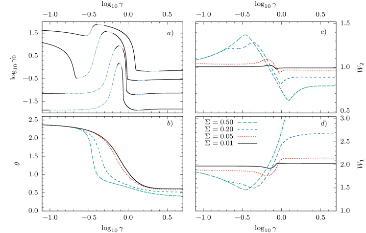
Figure 1: The evolution of the ND model assuming homogeneous flow, for fixed applied stress, $\theta_{0}=2.4$, $\epsilon=0.01$ and $r=2$. (a) shows the strain rate evolution. The solid black lines are stable flow, and the dashed regions are unstable. The blue long dashing has $d\dot{\gamma}/d\gamma>0$, and the red dashed region has $d\dot{\gamma}/d\gamma<0$ (Eq. (50) and (51)) . (b) shows the evolution of the director angle, (c) and (d) show the $W_{2}$ and $W_{1}$ components of the polymer shape tensor. Note that (d) shows that $W_{1}$ shrinks before the director rotation, corresponding to compressing the polymers along their long axis. After rotation the polymers are then extended by the shear flow.

The fluid starts in an equilibrium state at $t=0$, and is subjected to a step $xy$ shear stress of magnitude $\Sigma_{0}$. The homogeneous shear rate that arises in response to this stress, $\dot{\gamma}_{0}(t)$, can be calculated by numerical solution of the ordinary differential equations (16, 17, 18) (setting $\mathcal{D}=0$) and substituting for $\dot{\gamma}$ using

$$\dot{\gamma}=\frac{(\Sigma-\sigma_{xy})}{\epsilon},$$ (48)

where $\sigma_{xy}$ can be found in terms of ${\mathbf{W}}$ from Eq.(8). LSA gives us the condition for the development of spatial fluctuations. The fluctuations around the base state obey Eq. (46). These fluctuations obey the same dynamical equation as the base state ${\mathbf{s}}_{0}$, so it can be shown that the condition for the growth of fluctuations is Adams et al. (2011)

$$\frac{d^{2}\dot{\gamma}_{0}}{dt^{2}}/\frac{d\dot{\gamma}_{0}}{dt}>0,$$ (49)

i.e. we are looking for both upward sloping and upward curving shear rate, or downward sloping and downward curving shear rate. The numerical results of this calculation can be most easily understood by plotting the shear rate as a function of strain, since $\dot{\gamma}=\dot{\gamma}(\gamma)$, for different total stress values. This condition can be converted to strain to give

$$\frac{d\dot{\gamma}}{d\gamma}>0\;\;\textrm{and}\;\;\frac{d^{2}\dot{\gamma}}{d\gamma^{2}}>-\frac{1}{\dot{\gamma}}\left(\frac{d\dot{\gamma}}{d\gamma}\right)^{2}$$ (50)

or

$$\frac{d\dot{\gamma}}{d\gamma}<0\;\;\textrm{and}\;\;\frac{d^{2}\dot{\gamma}}{d\gamma^{2}}<-\frac{1}{\dot{\gamma}}\left(\frac{d\dot{\gamma}}{d\gamma}\right)^{2}$$ (51)

The negative sloping and negative curvature condition is observed in the ND model (Moorcroft and Fielding comment that it is not observed in Giesekus or the Rolie-Poly model Moorcroft and Fielding (2014)). Note that the condition in strain variables here requires that the curvature with respect to strain be more negative for more steeply sloped curves as compared to the corresponding situation with positive curvature. This is evident in the following numerical calculations.

The constitutive equations in the eigenbasis for the ND model were solved using the NAG C library d02ejc NAG . This is an implementation of variable-step backward differentiation formulae for stiff ordinary differential equations. The stability of the system is sensitive to the initial orientation of the director $\theta_{0}$. For prolate polymer conformation ($r>1$) the director rotates towards the stable solution of Eq. (37). For director angles close to the stable solution there is no flow instability predicted by LSA. However, if the director angle is close to the unstable solution of Eq. (37) then there is a sharp peak in $\dot{\gamma}_{0}$. Fig. 1a) shows the shear rate as a function of strain for a variety of different total shear stresses, with a fixed starting angle of $\theta_{0}=2.4$. The unstable regions of this curve are highlighted with a dashed line. Note that there are small regions of negative curvature that are unstable for the ND model. However the instability arising from the preceding upward sloping and upward curving region of the shear rate would result in an inhomogeneous velocity profile, and make the underlying assumption of a spatially homogeneous state for subsequent regions of the curve invalid.

The peak in the strain can be understood from Eq. (48). As a result of the flow there is a component of the flow field that gradually rotates the director. However, due to the alignment of the director the corresponding polymer shear stress component $\sigma_{xy}$ gradually falls to zero as the director rotates, and so to maintain the fixed stress condition the shear rate $\dot{\gamma}$ increases. The peak in the shear rate occurs when $\sigma_{xy}=0$, where $\dot{\gamma}=\Sigma/\epsilon$. This expression corresponds to the peaks in strain rate in Fig. 1a). The associated realignment of the director is shown in Fig. 1b). The rapid reorientation of the director results in a stable angle of the director from Eq. (37), and resolves the unstable flow.

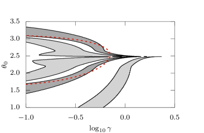
Figure 2: The stability of the homogeneous state at fixed stress with $\Sigma=0.1$, $r=2$ $\epsilon=0.01$ as a function of initial angle of the director $\theta_{0}$ and shear strain $\gamma$. The shaded area shows $\dddot{\gamma}/\ddot{\gamma}>0$, with light grey for $(\dot{\gamma},\dddot{\gamma})>0$ and dark grey for $(\dot{\gamma},\dddot{\gamma})<0$. The dashed (red) line shows the maximum strain of the soft mode of an LCE in Eq. (53).

The shear flow distorts the equilibrium polymer shape as the flow progresses. Initially the average conformation of the LCPs are prolate spheroids with their long axis parallel to the director. However for the LCPs in Fig. 1 they are compressed along ${\mathbf{n}}$ (i.e $W_{1}$) and elongated in the perpendicular direction (i.e. $W_{2}$), storing elastic energy, before reorientation (Fig. 1c) and d)). The rotation of the director then allows the polymers to release this elastic energy, and the flow field continues to stretch the polymers along the director.

The instability is sensitive to the initial orientation of the director. Fig. 2 shows the region of instability as a function of initial angle $\theta_{0}$ and $\gamma$ for $\Sigma=0.1$. The correspondence to Fig. 1 can be seen with the two bands for small strains corresponding to the leading and trailing edges of the peak in shear rate. The instability is strongest when the initial director angle is pointed away from the flow direction. Note that the initial angle $\theta_{0}$ where there is a cusp as a function of strain corresponds to $\dot{\theta}=0$ in the constitutive equations (Eq. (22, 23, 24)).

IV.1.1 Relation to soft elasticity

The shape of the shaded unstable regions in Fig. 2 can be understood by comparing them with the equilibrium model of liquid crystalline elastomers (LCEs), which is obtained in the elastic limit of the ND model. In this case an analytical expression for the expected value of this strain of the soft mode can be calculated from the trace formula used to describe LCEs. The free energy, $F$, here is given by

$$F=\textstyle{\frac{1}{2}}\mu\textrm{Tr}\left[\mbox{\boldmath{$\lambda$}}\cdot\mbox{\boldmath{$\ell$}}_{0}\cdot\mbox{\boldmath{$\lambda$}}\cdot\mbox{\boldmath{$\ell$}}^{-1}\right]$$ (52)

where $\mu$ is the shear modulus, $\lambda$ is the deformation matrix, $\mbox{\boldmath{$\ell$}}_{0}={\mathbf{I}}+(r-1){\mathbf{n}}_{0}{\mathbf{n}}_{0}$ is the initial polymer shape tensor, and $\mbox{\boldmath{$\ell$}}={\mathbf{I}}+\left(\frac{1}{r}-1\right){\mathbf{n}}{\mathbf{n}}$ is the current polymer shape tensor Warner and Terentjev (2003). We set ${\mathbf{n}}_{0}=(\cos\theta_{0},\sin\theta_{0},0)$, ${\mathbf{n}}=(\cos\theta,\sin\theta,0)$ and $\mbox{\boldmath{$\lambda$}}={\mathbf{I}}+\hat{{\mathbf{x}}}\hat{{\mathbf{y}}}\gamma_{0}$. The free energy $F$ is then minimised with respect to $\theta$ for a fixed strain $\gamma_{0}$ and initial angle $\theta_{0}$. It can be shown that this expression has minimum in $F$ for $\gamma_{0}=0$ and

$$\gamma_{0}=\frac{2(r-1)\sin 2\theta_{0}}{(r-1)\cos 2\theta_{0}-(r+1)}.$$ (53)

For the initial conditions in Fig. 1, this expression gives a value of $\textrm{log}_{10}\gamma_{0}\approx-0.15$ which coincides with the peak in the shear rate in Fig. 1.

Eq. (53) predicts that the position of the peak in the strain rate depends on the initial angle $\theta_{0}$. A contour of the strain as a function of the initial angle, $\theta_{0}$ is shown in Fig. 2. The maximum amplitude of $\gamma_{0}$ corresponds to the cusp shown in this figure.

IV.2 Step shear rate

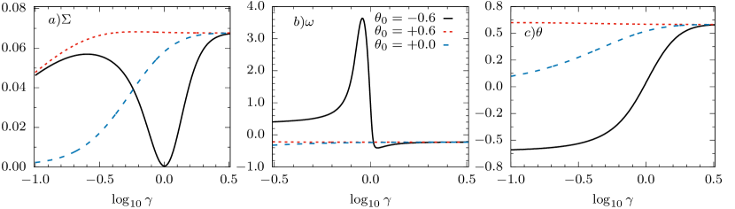
Figure 3: The evolution of a) the total stress, b) maximum eigenvalue $\omega$, and c) director angle for an imposed shear rate $\dot{\gamma}_{0}=0.1$, polymer anisotropy $r=2$ and initial director orientations of $\theta_{0}=-0.6,0.0,0.6$ (black solid, red dotted, and blue dashed lines respectively).

We now consider a step shear rate experiment. The fluid starts in its equilibrium state at $t=0$ and is then subjected to a shear rate $\dot{\gamma}$ for $t>0$. The stability of the homogeneous base state to spatially inhomogeneous flow can be found by analysing the eigenvalues of the matrix ${\mathbf{P}}$ given in Eq. (47). The behaviour of the fluid for starting angles of $\theta_{0}=0.6,0.0$ and $-0.6$ are shown in Fig. 3. The total shear stress is monotonically increasing for $\theta_{0}=0$ or $0.6$, and $\omega$ remains negative for all values of shear strain. No radical change of the director orientation is required here. However, for $\theta_{0}=-0.6\equiv\pi-0.6$ the director undergoes a large rotation towards the flow direction (solid black line in Fig. 3 c)). During the rotation there is a drop in the shear stress, and a simultaneous spike in the value of $\omega$, a sign of a spatial instability. This indicates that small perturbations of polymer stress components around the homogeneous base state should grow here. One difficulty with this eigenvalue analysis is that we do not know for how long or how positive the eigenvalues must be in order to cause a spatial instability. Previous analysis has looked at the integrated area of the positive region of $\omega$ Adams et al. (2011), however this is not particularly instructive. For larger values of shear rate the total stress dips to negative values for the homogeneous state. This is typical of the behaviour of LCEs during their deformation.

An alternative method of determining the stability of the fluid to fluctuations for imposed shear rate is presented in appendix C. The properties of the eigenvalues of this system of equations make it difficult to use the stability criterion of Moorcroft et al. Moorcroft and Fielding (2014). These properties are discussed in appendix D.

V Spatially resolved model

To understand the nature of the instabilities predicted from LSA we will solve the constitutive equations in Eq. (16), (17) and (18) for the 1D case of a planar shear between two infinite plates at $y=0$ and $y=1$. We will use Neumann boundary conditions at $y=0,1$ $\frac{\partial W_{\alpha\beta}}{\partial y}=0\,\forall\,\alpha,\beta$ for ${\mathbf{W}}$, while we will assume no wall slip and no penetration of the particles through the wall for the velocity i.e. ${\mathbf{v}}=v(y,t){\mathbf{x}}$. The effect of changing the boundary conditions in shear banding systems has been explored elsewhere Adams et al. (2008b).

In the creeping flow approximation we ignore inertia, so force balance reduces to Eq. (13). Since we only have spatial variation in the $y$-direction (i.e. $\nabla\equiv\hat{{\mathbf{y}}}\frac{\partial}{\partial y}$) then integrating Eq. (13) with respect to $y$ gives $\Sigma_{xy}(y,t)=\sigma_{xy}+\epsilon\dot{\gamma}=f(t)$, i.e. the total shear stress is the same at all points across the gap, though it can vary with time. We will use this condition in the fixed average shear rate case to calculate the local shear rate as follows

$$\Sigma_{xy}(t)=\sigma_{xy}+\epsilon\dot{\gamma}=\overline{\sigma_{xy}}+\epsilon\overline{\dot{\gamma}},$$ (54)

where the bar denotes the spatial average

$$\overline{\dot{\gamma}}=\int_{0}^{1}\dot{\gamma}(y,t)dy.$$ (55)

For a fixed total shear stress $\Sigma_{xy}$ the local shear rate is given by:

$$\dot{\gamma}(y,t)=(\Sigma_{xy}-\sigma_{xy}(y,t))/\epsilon.$$ (56)

The inhomogeneity that arises in the flow field can be quantified in many different ways, such as the difference between the maximum and minimum shear rates: $\dot{\gamma}_{\textrm{max}}-\dot{\gamma}_{\textrm{min}}$ Adams et al. (2011). We use here a more robust measure of the inhomogeneity that does not depend so critically on just two values of the shear rate:

$$\Delta\dot{\gamma}=\int_{0}^{1}\left|\dot{\gamma}(y)-\overline{\dot{\gamma}}\right|dy.$$ (57)

For a system with a uniform shear rate this will be zero, and it will be positive for non-uniform shear rate profiles.

V.1 Numerical scheme

For numerical solution of Eq. (16), (17) and (18) we use a finite difference scheme with two staggered uniform grids each with spacing $\Delta y$, $y_{n}=y_{0}+n\Delta y$. We use the full points $y_{0},y_{1}\ldots y_{N}$ for the velocity field $v_{x}(y,t)$ and the half-points $y_{1/2},y_{3/2}\ldots y_{N-1/2}$ for ${\mathbf{W}}$, $\sigma$ and $\dot{\gamma}$.

In order to integrate from time $n\Delta t$ to $(n+1)\Delta t$ we first use the values of $W^{(n)}_{xx},\,W^{(n)}_{xy},\,W^{(n)}_{yy}$ at the current time-step $n\Delta t$ to calculate the values of $\dot{\gamma}^{(n)}(y_{i/2},n\Delta t)$ with Eq. (54) for the fixed strain rate, and Eq. (56) for the fixed stress case. These are then used in the finite difference form of the constitutive equations which are integrated forwards in time using the Crank-Nicolson algorithm Press et al. (1993) to obtain $W^{(n+1)}_{xx},\,W^{(n+1)}_{xy},\,W^{(n+1)}_{yy}$ at the new time-step. In addition the values of $\dot{\gamma}^{(n)}(y,t)$ are integrated spatially to obtain the velocity at each full grid point $v^{(n)}_{x}(y_{i},n\Delta t)$.

For our chosen value of $\hat{D}=10^{-4}$ we expect a shear band to have a thickness $l\approx\sqrt{\hat{\cal{D}}}=10^{-2}$. In order to have roughly $10$ grid points on the interface we should then have $\Delta y\lesssim 10^{-3}$, i.e. we need $N\gtrsim 10^{3}$ grid points. We have tested our algorithm for convergence as we change both $\Delta t$ and $\Delta y$. To obtain stable and accurate results we find we need $\Delta t\approx\Delta y^{2}/(10\hat{\cal{D}})\approx 10^{-3}$.

V.2 Initial conditions

The initial conditions have a dramatic effect on the evolution of the system because they are amplified dramatically as a result of the flow instability. A small noise term was used to seed the initial configuration to make the calculations more reproducible. The noise was set using Fourier harmonics with random amplitudes. High frequency harmonics result in many interfaces developing, and a more complicated spatial structure, which eventually becomes uniform as the system evolves. To keep the spatial structure simple we used the following initial condition in start up from the relaxed state

$${\mathbf{W}}={\mbox{\boldmath{$\ell$}}}_{0}+U_{xy}(\hat{{\mathbf{x}}}\hat{{\mathbf{y}}}+\hat{{\mathbf{y}}}\hat{{\mathbf{x}}})$$ (58)

with the perturbing noise term

$$U_{xy}=\xi\cos\frac{\pi y}{L}.$$ (59)

It was found that a noise amplitude of $\xi=10^{-2}$ was adequate to trigger the instability reliably.

Note that the equations solved here are for a parallel plate rheometer. The curvature of the rheometer has been included elsewhere, and is found to break the symmetry of the system and determine where the high and low shear rate bands form Adams et al. (2008b).

V.3 Imposed average shear rate

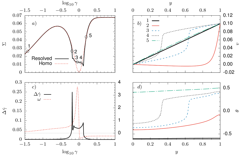
Figure 4: Spatially resolved model for imposed average shear rate $\overline{\dot{\gamma}}=0.1$, polymer anisotropy $r=2$, and initial director angle $\theta_{0}=-0.6$. a) Shear stress as a function of shear strain, b) velocity profile as a function of position $y$ at the time points labelled $1-5$ in a). The maximum real part of the eigenvalues, $\omega$, as a function of time (right hand $y$-axis), and shear rate inhomogeneity $\Delta\dot{\gamma}$ (left hand $y$-axis) are shown in c). The director angle is shown in d) for the corresponding lines shown in velocity profile plot b).

The typical results of the calculation for imposed average shear rate are shown in Fig. 4 for $\overline{\dot{\gamma}}=0.1$, for an initial director angle of $\theta_{0}=-0.6$, i.e. with the director tilted away from the flow direction. The shear stress in the spatially resolved model in Fig. 4 a) follows the homogeneous calculation initially. Once the director rotation starts then there is a sharp dip in the shear stress, where the spatially resolved model and the homogeneous model start to differ. The spatial shear rate then becomes inhomogeneous as shown by $\Delta\dot{\gamma}$ in Fig. 4 c). This coincides with the maximum eigenvalue of the stability matrix, $\omega$. The velocity profile is shown in Fig. 4 b) for various shear strain values indicated in a). They show a high strain rate band propagating across the rheometer gap. The high shear rate region corresponds to the rotation of the director as can be seen from Fig. 4 c).

This picture is shown more clearly in Fig. 5. Here the polymer conformation tensor ${\mathbf{W}}$ is represented by an ellipsoid. This illustrates the director orientation, and the local anisotropy. At the onset of rotation shown in a) almost the whole fluid becomes stationary, and a high strain rate region develops next to the wall. This high strain rate region propagates across the rheometer rotating the director. After the director has rotated the local strain rate drops dramatically, resulting in plug flow.

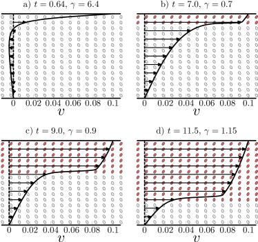
Figure 5: An illustration of the velocity profiles for imposed average shear rate $\bar{\dot{\gamma}}=0.1$, and initial director orientation $\theta_{0}=-0.6$. The velocity field and the orientation of the director are shown as a function of space various for different time points in (a-d). The regions with the director pointing in the flow direction are shown with dark (red) shaded ellipsoids, and those with the director oriented away from the flow direction are shown in light grey.

The mechanics of the director rotation can be seen clearly by plotting the director angle and the shear stress on the same axes, as shown in Fig. 6. The polymer component of shear stress $\sigma_{xy}$ drops dramatically at spatial point where the director is rotating. This drop in stress during director rotation is typical of liquid crystalline polymer systems. The total stress across the sample is fixed, so there is a corresponding rise in the shear rate, and hence the viscous component of the shear stress. The highly sheared region propagates across the gap causing director rotation.

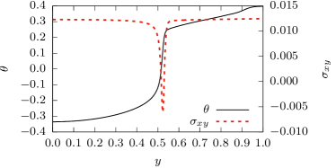
Figure 6: The spatial dependence of the director angle, the polymer stress $\sigma_{xy}$ for average shear rate $\overline{\dot{\gamma}}=0.1$, with initial condition $\theta_{0}=-0.6$, at the time point $t=1.0$, $\gamma=10.0$. Note that there is a sharp drop in the polymer stress where the director rotation occurs.

The director rotation is particularly pronounced when $\dot{\gamma}\sim 1$. For much higher shear rates the rotation front propagates very rapidly across the sample, and director rotation occurs simultaneously for all values of $y$. This is the elastic limit of the ND model. A range of flow behaviour is shown in Fig. 7 where the boundary between the rotated and the unrotated director regions is illustrated.

Figure 7: The position in the gap $y$ of the boundary between the region where the director points in the flow direction ($0<\theta<\pi/2$) as a function of strain $\gamma$ for initial director orientation $\theta_{0}=-0.6$, for different values of imposed average shear rate $\overline{\dot{\gamma}}$ shown on plots (a-d). Note that for high average shear rates the rotation of the director is almost simultaneous for all $y$.

For higher shear rates the flow profile can show recoil behaviour. This is shown in Fig. 8 for $\overline{\dot{\gamma}}=1$. At the onset of director rotation the drop in the shear stress from rotation requires a negative velocity in the rest of the sample to produce the required shear rate. The interface between the rotated and the unrotated phases is much more sharply defined here, resulting in plug flow – i.e. the whole rotated phase moves with the same velocity.

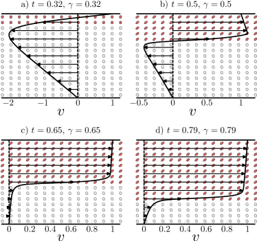
Figure 8: An illustration of the velocity profiles, and polymer shape tensor for $\overline{\dot{\gamma}}=1$ and $\theta_{0}=-0.6$. The time of each velocity profile is shown above each plot (a-d). The regions with the director pointing in the flow direction are shown with dark (red) shaded ellipsoids, and those with the director oriented away from the flow direction are shown in light grey.

V.4 Imposed shear stress

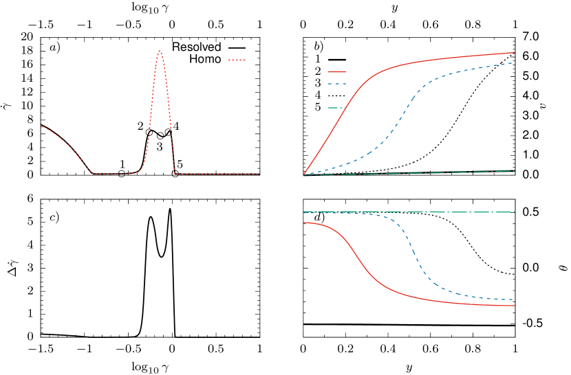
Figure 9: Spatially resolved calculations for imposed total shear stress $\Sigma=0.1$, initial director angle $\theta_{0}=-0.6$, and polymer anisotropy $r=2$. a) shows the average shear rate as a function of average shear strain for the spatially resolved and homogeneous calculations. b) shows the velocity profiles as a function of position across the gap, $y$, for the strain values indicated in a). c) shows the measure of inhomogeneity in shear rate $\Delta\dot{\gamma}$ as a function of average shear strain. d) shows the director angle as a function of spatial position $y$ for the corresponding strain values indicated in b).

Typical results of the spatially resolved calculation for fixed imposed shear are shown in Fig. 9. Here figure 9 a) shows the average shear rate for the spatially resolved and the spatially homogeneous calculations. They are identical for small strains. The degree of spatial inhomogeneity can be seen in 9 b). Once the velocity profile becomes inhomogeneous then the shear rates in a) differ – the spatially resolved system has a much lower average shear rate. The corresponding spatial profiles for the velocity and director angle are shown in b) and d) respectively. This shows that a high shear rate front propagates across the rheometer gap, accompanied by a rotation of the director. Once the director has rotated to the steady state value, then the average shear rate drops sharply, and is consistent with the spatially homogeneous results.

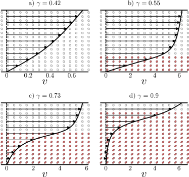
Figure 10: The velocity profiles at different values of average strain, $\gamma$ for an imposed total shear stress $\Sigma=0.1$, and initial director orientation $\theta_{0}=-0.6$. The ellipsoids indicate the conformation of the polymer. The angle of the principal axis corresponds to the director orientation. The regions with the director pointing in the flow direction are shown with dark (red) shaded ellipsoids, and those with the director oriented away from the flow direction are shown in light grey.

The velocity distribution and the polymer conformation are also shown in Fig. 10 for a range of different shear strains. Here it can be seen that the rotation front nucleates at the stationary plate of the rheometer ($y=0$) in b). This front is associated with a high shear rate that flips the orientation of the director. Once the director is rotated then it has a much lower velocity.

V.5 Flow reversal

The flow instability here in start up from rest depends critically on the initial condition. This is not practical for experimental systems. However, flow-reversal experiments are more practical to carry out in LCPs and have observed a change in the order parameter on flow reversal Ugaz et al. (2001); Mather et al. (2000). To illustrate the behaviour of the ND model under flow reversal the initial conditions were set with the director close to its steady state value: $\theta_{0}=0.6$. A fixed average shear rate of $\overline{\dot{\gamma}}=0.35$ was then applied from $t=0$ to $t=14$, at which point it was reversed to $\overline{\dot{\gamma}}=-0.35$. The results of the calculation are shown in Fig. 11. The resulting inhomogeneous velocity profile is very similar to that observed in start up shear – an inhomogeneous shear rate develops, then a high shear rate front propagates across the gap coinciding with director rotation. This may be a more practical experimental test for this theory.

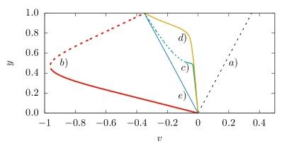
Figure 11: The velocity profiles for flow-reversal protocol with $\overline{\dot{\gamma}}=0.35$ for $t\leq 14$ and then $\overline{\dot{\gamma}}=-0.35$ for $t>14.0$. The lines labelled $a)-e)$ correspond to $t=13.0,16.1,16.4,16.8,16.9,$ and $20.0$ respectively. A solid line indicates that the director angle $\theta>\pi/2$ and a dashed line indicates that $\theta<\pi/2$.

VI Discussion

The ND constitutive model is a logical extension of the upper convected Maxwell (UCM) model, and describes semi-flexible LCPs, i.e. where each polymer chain can be distorted by the flow field. The calculations presented here show that this model has a transient flow instability to the formation of an inhomogeneous velocity profile under certain initial conditions. Its behaviour is qualitatively different to the shear banding observed in models that describe worm-like micellar solutions and polymer solutions, such as the Diffusive Johnson-Segalmann (DJS) model Olmsted et al. (2000), and the Vasquez-Cook-McKinley (VCM) model Zhou et al. (2008). These models are constructed to have shear banding in the steady state through a non-monotonic constitutive curve. The flow forms two bands – a high shear rate aligned phase and a low shear rate isotropic phase – with the average shear rate imposed on the system. The transient velocity profiles in models of polymer solutions such as the Diffusive Rolie-Poly (DRP) model Adams and Olmsted (2009) does not require a non-monotonic constitutive curve, but still has the same form of a high shear rate and a low shear rate band.

The ND model has a monotonic constitutive curve, but exhibits a different type of inhomogeneous velocity profile to transient shearbanding in the DRP model. A high shear rate front propagates across the rheometer gap and induces director rotation. This model is dominated by the elasticity of the polymer chains, hence the defect dynamics have no effect on the director distribution as observed in models of rod-like LCPs Grecov and Rey (2003). The ND model may exhibit even richer behaviour in higher dimensions, such as banding in the vorticity direction as well as the gradient direction, as has been found in the DJS model Fielding and Olmsted (2006).

There is both experimental evidence of mechanically induced phase transition in LCPs Mather et al. (1997), and consistent theoretical calculations Olmsted and Goldbart (1992, 1990). For semi-flexible LCPs the calculations here suggest that measurement of the order parameter should be done in such a way as to avoid averaging over the spatial variation in the director induced by the flow. This could arise if the measurements are taken by averaging across the gradient direction in the rheometer, for example by X-ray scattering with the beam passing through a Couette rheometer along the radial direction. A possible experimental test for this model is to use particle tracking velocimetry to measure the velocity distribution during start up flow, or a flow-reversal experiment. This experiment would reveal the inhomogenenous velocity profile predicted by the ND model.

The dynamics of the director rotation in this model are closely related to the formation of microstructure in liquid crystal elastomers Kundler and Finkelmann (1998). Here the typical geometry is an elongational deformation. Stripe domains of alternating rotation in the director field form. Imposed elongational flow in the ND model might produce microstructure with similar striped domains in the velocity profile.

Using mixtures of oblate and prolate chains could be modelled using the ND model to create LCPs with a tuneable flow aligning behaviour Kempe and Kornfield (2003).

VII Conclusion

We have analysed the nematic dumbbell model of Marrucci and Maffetone Maffettone and Marrucci (1992) with an additional polymer diffusion term, and a Newtonian solvent term. By using a linear stability analysis we determined the effect of spatial perturbations in the polymer stress components. These calculations were performed for both fixed shear strain rate, and fixed total shear stress. For initial conditions where the director is rotated away from the flow direction linear stability analysis shows that it is unstable. Spatially resolved calculations of the velocity profile show that there is some spatial structure in the velocity profile which corresponds to the reorientation of the director during the flow. The director rotation is confined to a front that propagates across the gap in the rheometer. For high imposed shear strain rates, or high total shear stress the rotation of the director occurs almost simultaneously across the whole sample. These calculations suggest that investigation of the spatial structure of the velocity field in the rheology of semi-flexible flow aligning liquid crystalline polymers may yield interesting results. One possible experimental test of this prediction is to use particle tracking velocimetry to measure the velocity profile of semi-flexible liquid crystalline polymers across the gap of a couette rheometer during a start up shear experiment.

Appendix A Elastic Limit

In the limit $t<<\tau_{\perp}$ the response of the system to an imposed shear strain should be purely elastic. We can thus ignore the viscous terms in Eq. (9). The constitutive equations are then:

$$\dot{W}_{xx} = 2W_{xy}\dot{\gamma}$$ (60)

$$\dot{W}_{yy} = 0$$ (61)

$$\dot{W}_{xy} = W_{yy}\dot{\gamma}.$$ (62)

Integrating these equations for a constant shear strain rate we obtain:

$$W_{xx}(t) = W_{xx}(0)+2\gamma(t)W_{xy}(0)+\gamma(t)^{2}W_{yy}(0)$$ (63)

$$W_{xy}(t) = W_{xy}(0)+\gamma(t)W_{yy}(0)$$ (64)

$$W_{yy}(t) = W_{yy}(0)$$ (65)

where the strain is given by $\gamma(t)=\dot{\gamma}t$. The director at a strain $\gamma$ is denoted by ${\mathbf{n}}=(\cos\theta,\sin\theta)$ and is the eigenvector associated with the largest eigenvalue of ${\mathbf{W}}$, it is simple to show that $\theta$ satisfies:

$$\tan 2\theta(t)=\frac{2W_{xy}(t)}{W_{xx}(t)-W_{yy}(t)}.$$ (66)

For the initial values we assume a nematic with anisotropy $r$ and initial director aligned along ${\mathbf{n}}_{0}=(\cos\theta_{0},\sin\theta_{0})$, thus:

$$W_{xx}(0) = 1+(r-1)\cos^{2}\theta_{0}$$ (67)

$$W_{xy}(0) = (r-1)\sin\theta_{0}\cos\theta_{0}$$ (68)

$$W_{yy}(0) = 1+(r-1)\sin^{2}\theta_{0}$$ (69)

using these values and solutions for $W_{xx}(t)$, $W_{xy}(t)$ and $W_{yy}(t)$ above we obtain the dependence of the angle $\theta$ on the shear strain $\gamma$ in the elastic limit

$$\tan 2\theta(\gamma)=\frac{\sin(2\theta_{0})-\gamma\cos(2\theta_{0})+\gamma\frac{(r+1)}{(r-1)}}{(1-\gamma^{2}/2)\cos(2\theta_{0})+\gamma\sin(2\theta_{0})+\frac{(r+1)}{(r-1)}\frac{\gamma^{2}}{2}}$$ (70)

This limit should describe the reorientation of the director for strains less than $\gamma\sim\dot{\gamma}\tau_{\perp}$. In Fig. 12 we plot the reorientation of a nematic with $\theta_{0}=0$ for various values of $\dot{\gamma}$ as a function of strain $\gamma$. As can be seen for small strains the reorientation follows the elastic limit (black line), but for strains $\gamma\gtrsim\dot{\gamma}\tau_{\perp}$ we start to see deviations from the elastic limit as stress begins to relax viscously.

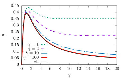
Figure 12: Reorientation of a dumbbell initially aligned along the flow direction in response to a shear strain $\gamma$ for various values of $\dot{\gamma}\tau_{\perp}$. The elastic limit (shown by the solid black line) corresponds to $\dot{\gamma}\tau_{\perp}\rightarrow\infty$.

Appendix B Small strain response

We work here in two dimensions, writing the director and its perpendicular component as

$${\mathbf{n}} = (\cos\theta,\sin\theta)$$ (71)

$${\mathbf{n}}_{\perp} = (-\sin\theta,\cos\theta)$$ (72)

$$\Rightarrow{\mathbf{W}} = (r+\delta){\mathbf{n}}{\mathbf{n}}+(1+\epsilon){\mathbf{n}}_{\perp}{\mathbf{n}}_{\perp}$$ (73)

where $\delta$ and $\epsilon$ are the leading order changes in the diagonal components for small amplitude shear. We will apply a velocity gradient given by ${\mathbf{K}}=\dot{\gamma}\hat{{\mathbf{x}}}\hat{{\mathbf{y}}}$. The components of the constitutive equations can then be calculated by taking the appropriate dot products ${\mathbf{n}}\cdot{\mathbf{W}}\cdot{\mathbf{n}}$, ${\mathbf{n}}\cdot{\mathbf{W}}\cdot{\mathbf{n}}_{\perp}$ and ${\mathbf{n}}_{\perp}\cdot{\mathbf{W}}\cdot{\mathbf{n}}_{\perp}$. Using this basis results in the following equation for the polymer stress $\mbox{\boldmath{$\sigma$}}=\mbox{\boldmath{$\ell$}}^{-1}\cdot{\mathbf{W}}$,

$$\sigma_{xy}=\frac{\delta-r\epsilon}{2r}\sin 2\theta$$ (74)

and the following equations result from the components of the constitutive equation.

$$\dot{\delta} = -\frac{2\delta}{r\tau}+\dot{\gamma}(r+\delta)\sin 2\theta$$ (75)

$$\dot{\epsilon} = -\frac{2\epsilon}{\tau}-\dot{\gamma}(1+\epsilon)\sin 2\theta$$ (76)

$$\dot{\theta} = \frac{1}{2}\dot{\gamma}\frac{1-r-\delta+\epsilon+(1+r+\delta+\epsilon)\cos 2\theta}{r+\delta-1-\epsilon}$$ (77)

These can be solved to find the leading order response for small deviations of $\theta$ from its starting orientation $\theta=\theta_{0}+\xi$ under oscillatory shear strain $\gamma(t)=\gamma_{0}\sin\omega t$. In this case

$$\dot{\xi} \approx \frac{\gamma_{0}(1-r+(1+r)\cos 2\theta_{0})}{2(r-1)}\omega\cos\omega t$$ (78)

$$- \gamma_{0}\delta\omega\cos\omega t\frac{\cos 2\theta_{0}}{(r-1)^{2}}+\gamma_{0}\epsilon\omega\cos\omega t\frac{r\cos 2\theta_{0}}{(r-1)^{2}}$$ (79)

$$- \xi\gamma_{0}\omega\cos\omega t\frac{(r+1)\sin 2\theta_{0}}{r-1}.$$ (80)

Note that when $\cos 2\theta_{0}=\frac{r-1}{r+1}$ then the leading order in $\xi$ is zero.

Leading order response is

$$\xi(t)=\frac{\gamma_{0}(1-r+(1+r)\cos 2\theta_{0})}{2(r-1)\omega}\omega\sin\omega t$$ (81)

Substituting this back into the equations for $\delta$ and $\epsilon$, we find the leading order response for the shear stress in the limit $t\rightarrow\infty$ (after the transient has dissipated).

$$\sigma_{xy} = \frac{\gamma_{0}\omega\sin^{2}2\theta_{0}}{(4+\omega^{2})(4+r^{2}\omega^{2})}\times$$ (82)

$$\left(\omega(2+r^{2}(2+\omega^{2}))\sin\omega t\right.$$

$$+ \left.(1+r)(4+r\omega^{2})\cos\omega t\right).$$

We can extract the storage and loss modulus from Eq. (82):

$$G^{\prime}(\omega) = \frac{\omega^{2}(2+r^{2}(2+\omega^{2}))}{(4+\omega^{2})(4+r^{2}\omega^{2})}\sin^{2}2\theta_{0}$$ (83)

$$G^{\prime\prime}(\omega) = \frac{\omega(r+1)}{4+\omega^{2}}\sin^{2}2\theta_{0}.$$ (84)

Note this material becomes soft (i.e. $G^{\prime}=G^{\prime\prime}=0$) when $\theta_{0}$ is small, but the analysis is not valid for $\theta_{0}=0,\pi/2$. This is the soft elastic response observed in LCEs as a result of the rotation of the director Warner and Terentjev (2003). The isotropic results $r=1$ of the Upper Convected Maxwell model can be recovered by setting $\theta_{0}=\pi/4$ and $r=1$.

When $\theta_{0}=0$ then the response becomes much softer and is no longer sinusoidal.

$$\sigma_{xy} = \frac{\gamma_{0}^{3}\omega\cos\omega t}{(r-1)^{2}(1+\omega^{2})(1+r^{2}\omega^{2})}\times$$ (85)

$$\left(\omega(1+r^{2}(1+2\omega^{2}))\sin 2\omega t\right.$$

$$\left.+(1+r)(1+r\omega^{2})\cos 2\omega t\right)$$

The material has no linear response regime here due to the soft rotation of the director. This contains both the $\omega t$ and $3\omega t$ harmonics at the same order in $\gamma_{0}$. This degeneracy in the model could be removed by including the response of the Newtonian solvent term, or by modifying the constitutive equation of the LCP to include imperfections such as the dispersity of the anisotropy as has been done for semi-soft LCEs.

For larger amplitude oscillatory shear the response is non-linear due to the rotation of the director during the flow.

Appendix C Integration of fluctuations

Figure 13: The integrated fluctuation in the shear rate $\delta\dot{\gamma}$ from Eq. (44) for $\theta_{0}=-0.6$. The lines correspond to $\log_{10}\delta\dot{\gamma}=-1,1,3,5,7,9$, for an initial amplitude of $\delta W_{ij}=10^{-3}$.

The extent of the growth in fluctuations during the shear flow can be measured using the shear rate fluctuations from Eq. (44). We can integrate the result over time (or equivalently strain). This approach was followed in Ref. Moorcroft and Fielding (2014). The solution of the constitutive equations was first calculated in the eigenbasis. The LSA was done in the Cartesian basis and the fluctuations in $\dot{\gamma}$ integrated using the initial conditions of $\delta W_{xx},\delta W_{xy}$ and $\delta W_{yy}$ set to $10^{-3}$. The NAG C library routine d02ejc was used to integrate these equations. Fig. 13 shows the result of this calculation for the ND model, for an unstable initial configuration of $\theta_{0}=-0.6$. As can be seen from the contours in this figure the fluctuations grow most strongly for $\dot{\gamma}\sim 1$. The cusp running down the contours arises from the change in sign of $\delta{\dot{\gamma}}$ during the calculation. The fluctuations eventually decay away indicating that the instability in this model is transient, and the steady state is spatially homogeneous.

Appendix D Properties of LSA eigenvalues

A general criterion for the determination of the stability of the flow, for the fixed shear rate case, based on LSA has been derived in Moorcroft and Fielding (2014):

$$\epsilon-G{\mathbf{p}}\cdot{\mathbf{M}}^{-1}\cdot{\mathbf{q}}<0.$$ (86)

Some of the assumptions used in developing this criterion are not satisfied by the ND model. Firstly it is assumed that the determinant of ${\mathbf{M}}$ in Eq. (45) obeys $(-1)^{D}|{\mathbf{M}}|<0$, where $D$ is the dimensionality of ${\mathbf{M}}$. Whilst it can be shown that the determinant is negative in equilibrium, it does change sign as the ND model evolves, and depends on the applied shear rate. The eigenvalues of ${\mathbf{M}}$ are all real for small values of $\dot{\gamma}\approx 0.1$. For larger values of shear rate there is a Hopf bifurcation, and corresponding complex eigenvalues. In this case the determinant changes sign from negative to positive, and then back to negative. This behaviour of the eigenvalues means that analysing the determinant of ${\mathbf{M}}$ (i.e. the product of the eigenvalues) is not enough to determine if one of them has changed sign. The real part of two of the three eigenvalues could change sign simultaneously (in the Hopf bifurcation), and leave the sign of the determinant unchanged. Secondly the determinant of ${\mathbf{P}}$ of Eq. (47) also shows a Hopf bifurcation. Fig. 14 shows the eigenvalues of ${\mathbf{P}}$. The shading here shows that there are regions of $0,1$ or $2$ eigenvalues that have positive real part respectively. Some of the regions with $0$ or $2$ eigenvalues of positive real part can have complex conjugate pairs of eigenvalues – a Hopf bifurcation. These regions are indicated by the black line.

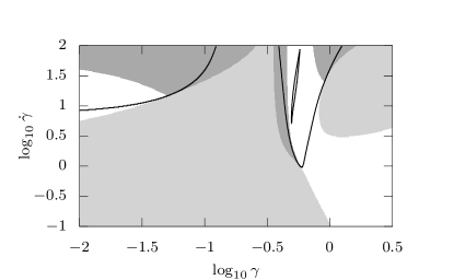
Figure 14: This figure shows the number of eigenvalues of the stability matrix ${\mathbf{P}}$ in Eq. (47) with positive real part for imposed average shear rate $\dot{\gamma}=0.1$ and $\theta=-0.6$. White corresponds to $0$ eigenvalues with positive real part, light grey to $1$ and dark grey to $2$. The black lines enclose the region where there is a Hopf bifurcation, i.e. two eigenvalues are complex conjugates pairs.

Fig. 15 shows the dependence of the maximum real part of the eigenvalue on the starting angle, $\theta_{0}$. The system is unstable for large strains in the region of $\theta_{0}>\pi/2$. There is a cusp for large strain at an angle corresponding to the unstable director orientation from the steady state solution.

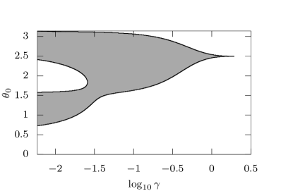
Figure 15: The shaded region shows where the maximum eigenvalue of ${\mathbf{P}}$ has a positive real part. The change in stability at $\gamma=0$ can be found from the $\dot{\theta}$ equation. The cusp for large $\gamma$ is the unstable result from the steady state equation.

References

- Rey and Denn (2002) A. D. Rey and M. M. Denn, Annual Review of Fluid Mechanics 34, 233 (2002).