Leading temperature dependence of the conductance in Kondo-correlated quantum dots

Abstract

Using renormalized perturbation theory in the Coulomb repulsion, we derive an analytical expression for the leading term in the temperature dependence of the conductance through a quantum dot described by the impurity Anderson model, in terms of the renormalized parameters of the model. Taking these parameters from the literature, we compare the results with published ones calculated using the numerical renormalization group obtaining a very good agreement. The approach is superior to alternative perturbative treatments. We compare in particular to the results of a simple interpolative perturbation approach.

I Introduction

The manifestations of the Kondo effect in transport through semiconducting gold ; cro ; gold2 ; wiel ; grobis ; keller and molecular leuen ; parks ; scott ; parks2 ; serge quantum dots (QDs) were a subject of great interest in the last years. The Kondo effect takes place when the occupancy of the isolated QD is such that its spin $S\neq 0$. For temperatures $T$ below the Kondo temperature $T_{K}$ this spin is totally or partially compensated by the conduction electrons of the leads leading to a many-body ground state with lower total spin. This implies a resonance at the Fermi energy in the spectral density of the dot state, that leads to an anomalous peak in the differential conductance $G(V)=dI/dV$ at zero bias voltage $V$, where $I$ is the current through the QD. For the simplest systems with one relevant level and $S=1/2$, these physical effects are usually well described by an impurity Anderson model (IAM), which contains the Kondo model as the limiting case in which valence fluctuations are absent hewson . The parameters of the IAM are the energy of the dot level $E_{d}$, the resonant level width $\Delta$ and the Coulomb repulsion $U$. The Kondo regime corresponds to $-E_{d},U+E_{d}\gg\Delta$ hewson .

In the Kondo limit, the properties of the IAM display universality. Physical observables are described by the same universal function, once the different physical magnitudes are scaled by $T_{K}$. For example, it has been shown that for $T\ll T_{K}$, the conductance $G(V,B)$ as a function of $V$ and magnetic field $B$, as well as the magnetization are universal functions of $eV/(k_{B}T_{K})$ and $\mu_{B}B/(k_{B}T_{K})$ for max$(eV,\mu_{B}B\gg k_{B}T_{K}$ rosch . In the opposite limit of small $V$ and $T$, Oguri ogu1 ; ogu2 has determined the scaling of $G(V,T)$ for $B=0$ up to second order in $T$ and $V$ for the symmetric IAM (SIAM) in which $E_{d}=-U/2$ using a Fermi liquid approach, extending to finite $V$ the renormalized perturbation theory (RPT) in $U$ developed by Hewson hew and using Ward identities. The result is given as an exact analytical expression in terms of renormalized parameters $\widetilde{\Delta}\sim k_{B}T_{K}$ and $\widetilde{U}$.

More recent experimental studies for the scaling properties of $G(V,T)$ for small $V$ and $T$ grobis ; scott stimulated further theoretical work on the subject rinc ; rati ; roura ; bal ; sela ; sca ; mu ; merker ; cb ; ng ; jpcs ; hanl ; oh using different approximations, like RPT rinc , $1/N$ expansion rati , non-crossing approximation roura , or decoupling of equations of motion bal . While the results for the Kondo model have been extended to SU(N) symmetry hanl , to fit experiment, calculations need to include some degree of valence fluctuations rinc ; roura suggesting that one has to go beyond the Kondo model and use the IAM for a quantitative description. The effect of asymmetric coupling to the left and right leads and asymmetric drop in the bias voltage has been calculated up to second order in $T$ and $V$ using Fermi liquid approaches, for the SIAM rinc ; sela ; sca . The more general expression was given first by Sela and Malecki sela and reproduced using RPT sca . These results are exact up to terms of total second order in $V$ and $T$.

Some of these results of RPT were extended for $E_{d}\neq-U/2$ using two different approaches. One of them starts from renormalized parameters of the IAM, $\widetilde{\Delta}$, $\widetilde{U}$ and $\widetilde{E}_{d}$ sca ; ng . The other starts from $\widetilde{\Delta}$ and $\widetilde{U}$ for the symmetric case $E_{d}=-U/2$ (for which $\widetilde{E}_{d}=0$) and performs another perturbation expansion around this point mu . The authors call this approach renormalized superperturbation theory (rSPT) jpcs . A controversy between the authors of both approaches exist for finite voltage $V$ ng ; jpcs ; com3 , but this does not affect equilibrium properties ($V=0$) like the one discussed here. In the last years also higher-order Fermi-liquid corrections away from half filling were calculated oh .

In Ref. mu an analytical expression using rSTP was obtained for the coefficient $c_{T}$ for the expansion for small $T$ and $V=0$ of the condunctance: $G(T)=G(0)[1-c_{T}(T/T_{K})^{2}]$. This result was compared with a fit of $G(T)$ for small $T$ obtained using the numerical renormalization group (NRG) merker . The comparison was poor, and rapidly deteriorates with increasing $U$. For $U=3\Delta$ the rSPT expression for $c_{T}$ increases as $E_{d}$ increases from the symmetric point $E_{d}=-U/2$, while the NRG result decreases. Later the authors included ladder diagrams in their rSPT approach (at the cost of losing an analytical expression) obtaining a considerable improvement jpcs . However still for $U=3\Delta$ and $E_{d}>-0.6\Delta$ the comparison is rather poor. Furthermore, the fact that the rSPT results presented are limited to $U\leq\Delta$ is a shortcoming for two reasons. First, the Kondo regime $-E_{d},U+E_{d}\gg\Delta$ is not reached. In the Kondo regime, the spectral density at the dot has in addition to the Kondo peak near the Fermi energy $\epsilon_{F}$, two charge-transfer peaks at energies near $E_{d}-\epsilon_{F}$ and $E_{d}+U-\epsilon_{F}$ of total width $4\Delta$ pru ; logan ; capac ; anchos . Then for $U=3\Delta$ even in the symmetric case, the Kondo peak is merged with one charge-transfer peak and valence fluctuations are important. Second, for small $U$, simple ordinary (not renormalized) perturbation theory up to second order $U$ yos ; hz ; hor has been successful for different problems levy ; kk ; nov . In particular, self-consistent interpolation schemes levy ; kk ; none permit to extend the validity of the results for $U$ as large as a few $\Delta$ depending on the problem. The interpolative perturbation approach (IPA) proposed in Ref. kk , and extended to finite magnetic field in Ref. none has been applied to the coefficient $c_{B}$ of the expansion of the conductance with magnetic field $G(B)=G(0)[1-c_{B}(g\mu_{B}B/k_{B}T_{K})^{2}]$ cb ; com3 leading results superior to those of the rSPT including ladder diagrams com3 . This IPA requires to satisfy selfconsistently the Friedel sum rule lan to each spin lady ; none . While this rule cannot be extended to finite temperature $T$, we have explored a simple extension for $T\rightarrow 0$, as explained in Section 3.

In this work, using RPT we derive an analytical (although lengthy) expression of the coefficient $c_{T}$ for the temperature expansion of the conductance, in terms of the renormalized parameters of the model $\widetilde{\Delta}$, $\widetilde{E}_{d}$ and $\widetilde{U}$. Taking tabulated values of these parameters from the literature for several values of the original parameters of the model, we obtain the corresponding $c_{T}$ and compare them with published NRG results. The agreement is excellent for most of the calculated points. The results can be rather easily extended for other sets of parameters in comparison with NRG for dynamical quantities. We also calculated $c_{T}$ within the IPA and compared with the other approaches.

In Section II, we explain briefly the RPT for the calculation of the Green functions and in particular the spectral density of impurity states and its expansion for $V=B=0$ and small $\omega$ and $T$. The expression of $c_{T}$ is given in Section II.4. The comparison with NRG and IPA results is presented in Section III. Section IV contains a discussion.

II Formalism

II.1 Hamiltonian

In the most general case, the model describes a QD interacting with two conducting leads, one at the left and one at the right, with chemical potentials $\mu_{L}$ and $\mu_{R}$ respectively, with $\mu_{L}$-$\mu_{R}=eV$. The system is at temperature $T$ in presence of a magnetic field $B$. For the sake of completeness we begin discussing the general case, and later we take $V=B=0$. The dot level has an on-site energy $E_{d}$ controlled by a gate voltage and an on-site repulsion $U.$ The Hamiltonian is that of the IAM

$$H = \sum_{k\nu\sigma}\varepsilon_{k\nu}c_{k\nu\sigma}^{\dagger}c_{k\nu\sigma}+\sum_{\sigma}E_{d}^{\sigma}n_{d\sigma}$$ (1)

$$+\sum_{k\nu\sigma}(V_{k\nu}c_{k\nu\sigma}^{\dagger}d_{\sigma}+{\rm H.c.})+Un_{d\uparrow}n_{d\downarrow}.$$

Here $\nu=L,R$ refers to the left and right leads and the operator $c_{k\nu\sigma}^{\dagger}$ creates an electron in the state with wave vector $k$ and spin $\sigma$ at the lead $\nu$, Similarly $d_{\sigma}^{\dagger}$ creates an electron with spin $\sigma$ at the QD. The number operator $n_{d\sigma}=d_{\sigma}^{\dagger}d_{\sigma}$ and $E_{d}^{\sigma}=E_{d}-\sigma\mu_{B}B$. We assume coupling to the leads $\Delta_{\nu}=\pi\sum_{k}|V_{k\nu}|^{2}\delta(\omega-\varepsilon_{k\nu})=\beta_{\nu}\Delta$ independent of energy, and define the total resonant level width $\Delta=\Delta_{L}+\Delta_{R}$.

II.2 Green function within renormalized perturbation theory

For a symmetric flat band of conduction states and constant $\Delta$ as we have assumed, the retarded Green function of the QD level for spin $\sigma$ can in general be written as

$$G_{d\sigma}(\omega)=\frac{1}{\omega-E_{d}^{\sigma}+i\Delta-\Sigma_{\sigma}(\omega)},$$ (2)

where $\Sigma_{\sigma}(\omega)$ is the (unknown) retarded self energy.

The basic idea of RPT is to reorganize the perturbation expansion in terms of fully dressed quasiparticles in a Fermi liquid picture hew . The parameters of the original model are renormalized and the renormalized values $\widetilde{\Delta}$, $\widetilde{U}$ and $\widetilde{E}_{d}^{\sigma}$ can be calculated exactly from Bethe ansatz results tsve ; tsve2 ; bethe , or accurately using NRG. One of the main advantages is that the renormalized expansion parameter $u=\widetilde{U}/(\pi\widetilde{\Delta})$ is small. In general $u\lesssim 1$. In the following we set the origin of one-particle energies at the Fermi level ($\epsilon_{F}=0$). Within RPT, the low-energy part of $G_{d\sigma}(\omega)$ is approximated expanding the denominator around $\omega=\epsilon_{F}=0$, for $V=T=0.$hew ; ng

$$G_{d\sigma}(\omega)\simeq\frac{z}{\omega-\widetilde{E}_{d}^{\sigma}+i\widetilde{\Delta}-\widetilde{\Sigma}_{\sigma}(\omega)},$$ (3)

where $z=[1-\partial\Sigma_{\sigma}(\omega)/\partial\omega|_{\omega=0}]^{-1}$ is the quasiparticle weight, $\widetilde{\Delta}=z\Delta$ is the renormalized resonant level width, $\widetilde{E}_{d}=z[E_{d}+\Sigma_{\sigma}(0)]$ is the renormalized level energy and

$$\widetilde{\Sigma}_{\sigma}(\omega)=z[\Sigma_{\sigma}(\omega)-\Sigma_{\sigma}(0)-\omega\partial\Sigma_{\sigma}(\omega)/\partial\omega|_{\omega=0}].$$ (4)

We emphasize that $\Sigma_{\sigma}(0)$ and $\partial\Sigma_{\sigma}(\omega)/\partial\omega|_{\omega=0}$ are calculated at $V=T=\omega=0$.com3

The renormalized Coulomb repulsion $\widetilde{U}$ is given by a vertex function ogu1 ; ogu2 ; hew .

The spectral density of $d$ electrons is

$$\rho_{\sigma}(\omega)=-{\rm Im}G_{d\sigma}(\omega)/\pi.$$ (5)

The free quasiparticle spectral density of $d$ electrons is given by

$$\widetilde{\rho}_{0}^{\sigma}(\omega)=\frac{\widetilde{\Delta}/\pi}{(\omega-\widetilde{E}_{d}^{\sigma})^{2}+\widetilde{\Delta}^{2}}.$$ (6)

Using Friedel sum rule lan ; lady one has

$$\pi\Delta\rho_{\sigma}(0)=\pi\widetilde{\Delta}\widetilde{\rho}_{0}^{\sigma}(0)=\sin^{2}(\pi\langle n_{d\sigma}\rangle).$$ (7)

Thus, knowing the occupancies $\langle n_{d\sigma}\rangle$ experimentally or by a Bette ansatz calculation for example, one can determine the ratios $\widetilde{E}_{d}^{\sigma}/\widetilde{\Delta}=\cot(\pi\langle n_{d\sigma}\rangle)$. The ratio $\widetilde{U}/\widetilde{\Delta}$ can be obtained from the expression of the impurity contribution to magnetic susceptibility at zero temperature hew

$$\chi=(g\mu_{B})^{2}\widetilde{\rho}_{0}(0)(1+\widetilde{U}\widetilde{\rho}_{0}(0))/2,$$ (8)

where $\widetilde{\rho}_{0}(\omega)=\widetilde{\rho}_{0}^{\uparrow}(\omega)=\widetilde{\rho}_{0}^{\downarrow}(\omega)$ for $B=0$ and $\widetilde{\Delta}$ can be obtained either from the linear term $\gamma_{C}$ in the impurity contribution to the specific heat hew

$$\widetilde{\Delta}=\frac{2\pi k_{B}^{2}}{3\gamma_{C}}\sum_{\sigma}\sin^{2}(\pi\langle n_{d\sigma}\rangle),$$ (9)

or approximately in RPT from the half-width at half maximum of the Kondo peak in $\rho_{\sigma}(\omega)$ cb .

To obtain the spectral density $\rho_{\sigma}(\omega)$ out of the point $\omega=T=V=0$, we need an approximation for $\widetilde{\Sigma}_{\sigma}(\omega)$. As in previous works rinc ; cb ; ng we use

$$\widetilde{\Sigma}_{\sigma}(\omega)=\widetilde{\Sigma}_{\sigma}^{2}(\omega)-\widetilde{\Sigma}_{\sigma}^{2}(0)-\omega\partial\widetilde{\Sigma}_{\sigma}^{2}/\partial\omega|_{\omega=0},$$ (10)

where $\widetilde{\Sigma}_{\sigma}^{2}(\omega)$ is obtained using perturbation theory up to second order in $\widetilde{U}$, using the free quasiparticle spectral density $\widetilde{\rho}_{0}^{\sigma}(\omega)$ [or the corresponding Green function $1/(\omega-\widetilde{E}_{d}^{\sigma}+i\widetilde{\Delta})$]. Since the constant first-order term vanishes in Eq. (10), a possible expression for $\widetilde{\Sigma}_{\sigma}^{2}(\omega)$ is none

$$\Sigma_{\uparrow}^{2}(\omega) = \widetilde{U}^{2}\int d\epsilon_{1}d\epsilon_{2}d\epsilon_{3}\frac{\widetilde{\rho}_{0}^{\uparrow}(\epsilon_{1})\widetilde{\rho}_{0}^{\downarrow}(\epsilon_{2})\widetilde{\rho}_{0}^{\downarrow}(\epsilon_{3})}{\omega+\epsilon_{3}-\epsilon_{1}-\epsilon_{2}+i\eta}$$ (11)

$$\times[(1-\tilde{f}(\epsilon_{1}))(1-\tilde{f}(\epsilon_{2}))\tilde{f}(\epsilon_{3})$$

$$+\tilde{f}(\epsilon_{1})\tilde{f}(\epsilon_{2})(1-\tilde{f}(\epsilon_{3}))],$$

where $\tilde{f}(\omega)=\sum_{\nu}\beta_{\nu}f(\omega-\mu_{\nu})$, with $f(\omega)$ the Fermi function, and the same interchanging spin up and down.

The lesser and greater Green functions are defined similarly ng .

II.3 Expansion of the renormalized retarded self energy

In the following, we take $V=B=0.$ Then $\widetilde{E}_{d}^{\sigma}=\widetilde{E}_{d}$ independent of $\sigma$. Borrowing results from Ref. hz for the expansion of $\widetilde{\Sigma}_{\sigma}^{2}(\omega)$ up to total second order in $\omega$ and $T$, and inserting them in Eq. (10) we obtain

$$\widetilde{\Sigma}_{\sigma}(\omega)=-u^{2}\frac{\alpha\omega^{2}+\beta(\pi k_{B}T)^{2}+i\gamma[\omega^{2}+(\pi k_{B}T)^{2}]}{\widetilde{\Delta}},$$ (12)

where we define

$$u = \frac{\widetilde{U}}{\pi\widetilde{\Delta}}{\rm,}\epsilon=\frac{\widetilde{E}_{d}}{\widetilde{\Delta}},$$

$$s = \sin(\pi\langle n_{d\sigma}\rangle)=\frac{\widetilde{\Delta}}{\sqrt{\widetilde{E}_{d}^{2}+\widetilde{\Delta}^{2}}},$$

$$c = \cos(\pi\langle n_{d\sigma}\rangle),$$ (13)

and the coefficients $\alpha$, $\beta$, and $\gamma$ are given by

$$\alpha = s^{4}(t_{1}+t_{2}),$$

$$t_{1} = \frac{\arctan(\epsilon)/\epsilon-s^{2}}{4\epsilon},$$

$$t_{2} = \arctan(\epsilon)[9/4+2\epsilon\arctan(\epsilon)]$$

$$+\epsilon s^{2}[\frac{13-3\pi^{2}+(\pi\epsilon)^{2}}{4}$$

$$+(1-3\epsilon^{2})g(\epsilon)],$$

$$g(\epsilon) = \frac{1}{\epsilon}\int\limits_{0}^{\epsilon}dt[\arctan^{2}(t)$$ (14)

$$+\frac{2}{t}\arctan^{2}(t)],$$

$$\beta=\frac{s^{2}}{3}[t_{1}(1+5\epsilon^{2})-\frac{\epsilon s^{2}}{2}],$$ (15)

$$\gamma=\frac{s^{4}}{2}.$$ (16)

II.4 Conductance as a function of temperature

In linear response ($V\rightarrow 0$) and for $B=0$, the conductance is given by meir

$$G(T)=C\int d\omega\rho_{\sigma}(\omega,T)\left(-\frac{\partial f(\omega)}{\partial\omega}\right),$$ (17)

where $C$ is a constant that depends on the couplings $\Delta_{L}$ and $\Delta_{R}$.

Up to second order in the temperature $T$, using the Sommerfeld expansion one has

$$G(T)\simeq C[\rho_{\sigma}(0,T)+\frac{(\pi k_{B}T)^{2}}{6}\frac{\partial^{2}\rho_{\sigma}(\omega,0)}{\partial\omega^{2}}|_{\omega=0}.$$ (18)

Using Eqs. (3), (5), (12), (13), (14), (15), (16), and (18) we obtain after some algebra the desired expression for the leading temperature dependence of the equilibrium conductance

$$\frac{G(T)}{G(0)} = 1+\left(\frac{\pi k_{B}T}{\widetilde{\Delta}}\right)^{2}[\frac{s^{2}}{3}(4c^{2}-1)$$ (19)

$$+u^{2}\{2\left(\frac{\alpha}{3}+\beta\right)sc+\frac{4\gamma}{3}(1-2s^{2})\}].$$

III Comparison with NRG for dynamical quantities and IPA

In Ref. merker , the coefficient $c_{T}$ was defined as

$$\frac{G(T)}{G(0)}=1-c_{T}\left(\frac{T}{T_{0}}\right)^{2},$$ (20)

where $T_{0}$ is of the order of the Kondo temperature and defined in terms of the magnetic susceptibility $\chi$ by

$$T_{0}=\frac{\left(g\mu_{B}\right)^{2}}{4k_{B}\chi}.$$ (21)

Eqs. (6) and (8) permit to express $T_{0}$ in terms of the renormalized parameters. For $-E_{d}=U/2\rightarrow\infty$, $T_{0}=\pi\widetilde{\Delta}/(4k_{B})$ hew and $c_{T}=\pi^{4}/16\approx 6.09$ ogu1 ; ogu2 . The values of the renormalized parameters parameters were calculated in Ref. cb following the procedure explained by Hewson et al. hom . They are reproduced in Table 1 for the ease of the reader. The original parameters include $U=8\Delta$ (for which the system is in the Kondo regime near the symmetric point $E_{d}=-U/4$), and $U\rightarrow+\infty$ which is more realistic for several molecular QDs serge . Using these renormalized parameters, we have calculated $c_{T}$ using the expression of the previous section. The results are shown in Fig. 1.

Table 1: Renormalized parameters $\widetilde{\Delta}/\Delta$, $\epsilon=\widetilde{E}_{d}/\widetilde{\Delta}$ and $u=\widetilde{U}/(\pi\widetilde{\Delta})$ obtained from NRG+RPT for several values of $U/\Delta$ and $E_{d}/\Delta$ cb .

$U/\Delta$	$E_{d}/\Delta$	$\widetilde{\Delta}/\Delta$	$\epsilon$	$u$
3	-1.5	0.639	0	0.738
3	-1	0.671	0.196	0.732
3	-0.5	0.754	0.421	0.716
3	0	0.845	0.700	0.698
8	-4	0.120	0	0.985
8	-3	0.143	0.101	0.987
8	-2	0.235	0.247	1.004
8	-1	0.457	0.510	1.040
8	-0.5	0.609	0.715	1.060
8	0	0.746	0.977	1.081
$+\infty$	-6	$2.51\times 10^{-4}$	0.0937	1.009
$+\infty$	-5	$1.21\times 10^{-3}$	0.118	1.014
$+\infty$	-4	$5.79\times 10^{-3}$	0.160	1.025
$+\infty$	-3	0.0270	0.243	1.054
$+\infty$	-2	0.115	0.416	1.136
$+\infty$	-1	0.356	0.766	1.317
$+\infty$	0	0.640	1.338	1.594

We also show $c_{T}$ for the same values of $U$ as those in Table 1 reported in Fig. 5 of Ref. merker . In that work, $c_{T}$ has been extracted from a fit to Eq. (20) of several low-temperature values (in the range $10^{-5}T_{0}\leq T\leq 0.02T_{0}$) of the conductance $G(T)$ obtained using an NRG for dynamical quantities developed in Ref. yso . In addition two values for $z$-averaging were used merker .

For a moderate value of $U=3\Delta$, we also show the results of the IPA. These were obtained with the following procedure. First we used for the self-energy the result based on second-order perturbation theory at $T=V=0$ and finite magnetic field $B$, as in Refs. none . The unperturbed Green functions

$$G^{0}_{d\sigma}(\omega)=\frac{1}{\omega-\varepsilon_{d}^{\sigma}+i\Delta},$$ (22)

corresponding to the unperturbed Hamiltonian

$$H_{0}=H-\sum_{\sigma}(E_{d}^{\sigma}-\varepsilon_{d}^{\sigma})n_{d\sigma}-Un_{d\uparrow}n_{d\downarrow},$$ (23)

are calculated with effective on-site energies $\varepsilon_{d}^{\sigma}$ determined self consistently to satisfy the Friedel sum rule for both spins lady . From this calculations we extract $\varepsilon_{d}=\varepsilon_{d}^{\uparrow}=\varepsilon_{d}^{\downarrow}$ for $B=0$ and the magnetic susceptibility from numerical differentiation of the magnetization. Using Eq. (21) $T_{0}$ is obtained. Then, we calculate the IPA self-energy at finite temperature keeping $\varepsilon_{d}$ fixed, and fit the low-$T$ results to a quadratic dependence.

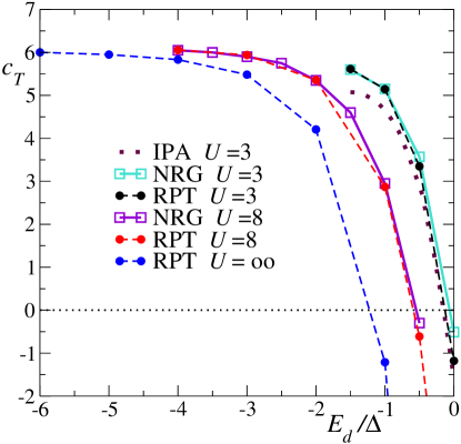
Figure 1: Coefficient $c_{T}$ of Eq. (20) vs $E_{d}$ for several values of $U$.

Since $c_{T}$ has the same value replacing $E_{d}$ by $U-E_{d}$ we represent in Fig. 1 only $E_{d}\geq-U/2$. It is apparent that $c_{T}$ decreases monotonically showing a downward curvature with increasing (or decreasing) $E_{d}$ starting from the symmetric point $E_{d}=-U/2$, becoming negative for $E_{d}\sim 0$.

It is clear that the comparison between RPT and NRG results are very good. For positive $c_{T}$ the difference is of the order of the symbol size and increases as the on-site energy $E_{d}$ is moved away from the symmetric point. For $U=3\Delta$ the maximum difference between the values included in the figure is 0.67 for $E_{d}=0$ (12 % of the maximum value $c_{T}=5.61$ for $E_{d}=-U/2$).

In Ref. merker also the coefficient $c_{T}^{\prime}$ was introduced which differs from $c_{T}$ in the fact that the characteristic temperature $T_{0}$ was taken always as that of the symmetric point $T_{0}^{\rm sym}\leq T_{0}$. The relation between both coefficients is

$$\frac{c_{T}^{\prime}}{c_{T}}=\left(\frac{T_{0}^{\rm sym}}{T_{0}}\right)^{2}.$$ (24)

The above mentioned difference in $c_{T}$ is reduced by a factor 0.18 ($k_{B}T_{0}=1.3468\Delta$, $k_{B}T_{0}^{\rm sym}=0.5775\Delta$) in $c^{\prime}_{T}$. Then, the maximum deviation in $c^{\prime}_{T}$ for $U=3\Delta$ is below 0.1. In Ref. jpcs , a comparison between result of $c^{\prime}_{T}$ calculated with NRG and rSPT including ladder diagrams was presented for $U\leq 3\Delta$. From Fig. 1 of Ref. jpcs , it is clear that the deviation of both results is already larger than 0.8 for $U=3\Delta$ and $E_{d}=-0.3\Delta$. This indicates that our RPT results for $U=3\Delta$ are nearly an order of magnitude more precise near $E_{d}=0$. Note that the rSPT results depend on two parameters, $\widetilde{\Delta}$, $\widetilde{U}$ for $E_{d}=-U/2$, while in our RPT approach one has in addition $\widetilde{E}_{d}$ and all parameters depend on $E_{d}$.

For $U=3\Delta$ we also show the results obtained using the IPA. In contrast to RPT and rSPT, the results do not depend on renormalized parameters. As a consequence, while RPT and rSPT give by construction the exact result at the symmetric point $E_{d}=-U/2$ taking known values of $\widetilde{\Delta}$ and $\widetilde{U}$ with $\widetilde{E}_{d}=0$, IPA deviates from the correct result. This is due to its inaccuracy in the calculation of the magnetic susceptibility (which determines the energy scale $T_{0}$), underestimated by 8 % and also an underestimation of the curvature of $G(T)$. The accuracy of the IPA increases away from the symmetric point, and taking into accounts its simplicity, the IPA provides a rather good semiquantitative description for $U=3\Delta$ (or lower), although $c_{T}$ continues underestimated in the whole range of $E_{d}$. The IPA seems to be better than the rSPT near the intermediate valence region.

The comparison between RPT and NRG for $U=8\Delta$ shows that the agreement does not deteriorate with increasing $U$ in contrast to the case of IPA cb or rSPT merker ; jpcs ; com3 . For example, the underestimation of the magnetic susceptibility at the symmetric point by the IPA increases to 15 % for $U=4\Delta$, while it is only 1.4 % for $U=2\Delta$.

IV Summary and discussion

Using renormalized perturbation theory (RPT), we have provided an analytical expression for the coefficient of the leading temperature dependence of the conductance through a quantum dot, in terms of the renormalized parameters of the impurity Anderson model $\widetilde{\Delta}$, $\widetilde{E}_{d}$ and $\widetilde{U}$. The expression is given by Eq. (19) where the different coefficients are defined by Eqs. (13), (14), (15) and (16). Using Eqs. (20) and (21) the coefficient $c_{T}$ defined previously merker is immediately obtained, and also $c^{\prime}_{T}$ [see Eq. (24)] which uses a fixed Kondo scale evaluated at $E_{d}=-U/2$. Although the expression is lengthy it can be easily evaluated. The most difficult task is a one-dimensional integration [last Eq. (14)]. The renormalized parameters can be easily obtained from the spectrum of an NRG calculation hom or from the calculation of static quantities with Bethe ansatz tsve ; tsve2 ; bethe , or from experiment. Refs. tsve ; tsve2 provide analytical expressions for the occupancy, magnetic susceptibility and specific heat, from which the renormalized parameters can be calculated using Eqs. (5) to (9). Some tricks to evaluate integrals that enter these expressions are given in the appendix of Ref. anda .

The calculation of dynamical quantities like the conductance is not possible with Bethe ansatz, and much more complicated within NRG hof ; bulla . To calculate $c_{T}$ directly within NRG for dynamical properties required several calculations at different temperatures within an optimized range of temperatures and for two different logarithmic discretizations ($z$-averaging) merker . We would like to notice that even the calculation of the static magnetic susceptibility $\chi$ [which determines $T_{0}$, see Eq. (21)] within NRG is much easier determining first the renormalized parameters and then using Eq. (8), as done in Ref. cb . A direct calculation of $\chi$ using standard NRG well inside the Kondo regime displays oscillations with temperature and even negative values fang ; wong . A full density-matrix NRG was required to solve this problem fang , but this is not necessary to calculate the renormalized parameters hom .

Our calculation with RPT is therefore much easier than direct evaluation of the conductance using NRG. It also has the advantage over ordinary (not renormalized) perturbation approaches cb ; com3 , or the so called renormalized superperturbation theory (rSPT) including ladder diagrams jpcs that the results do not deteriorate rapidly with increasing $U$ allowing us to reach the Kondo regime $-E_{d},U+E_{d}\gg\Delta$.

Different approaches discussed here (RPT, rSPT, NRG, but not IPA) give the same correct value of $c_{T}$ at the symmetric point $E_{d}=-U/2$. Also by definition, $c_{T}$ and $c^{\prime}_{T}$ coincide at this point [see Eq. (24)] Out of this point, since $T_{0}$ can be considerably larger than $T_{0}^{\rm sym}$, the magnitude of $c^{\prime}_{T}$ is smaller or much smaller than $c_{T}$. From this analysis, it is clear that plotting $c_{T}$ instead of $c^{\prime}_{T}$ is more appropriate to see differences between different approaches. Moreover $T_{0}$ is directly related with the width of the Kondo peak in the spectral density of states $2\Delta_{\rho}$ (the ratio $\Delta_{\rho}/T_{0}$ has been calculated within RPT in Ref. cb ), which in turn is of the order of the width $2\Delta_{G}$ of the zero-bias anomaly in the conductance $G(V)$ capac , which is experimentally accessible. The ratio $\Delta_{G}/\Delta_{\rho}$ depends on the ratio of the couplings between left and right leads $\Delta_{L}/\Delta_{R}$ and has been calculated capac .

In the Kondo regime, an empirical formula that fits very well the NRG results for the temperature dependence of the conductance has been proposed. gg . It can be written in the form

$$G(T)=\frac{G(0)}{\left[1+(2^{1/s}-1)(T/T^{G}_{K})^{2}\right]^{s}},$$ (25)

where $s=0.22$ and $T^{G}_{K}$ (of the order of $T_{0}$) is the temperature at which the conductance falls to half of the zero temperature value: $G(T^{G}_{K})=G(0)/2$. One may wonder to which extent the expansion of this expression for $T\rightarrow 0$

$$\frac{G(T)}{G(0)} \approx 1-c_{E}\left(\frac{T}{T^{G}_{K}}\right)^{2}$$

$$c_{E} = s(2^{1/s}-1)\approx 4.92,$$ (26)

gives the correct $c_{T}=\pi^{4}/16\approx 6.09$ in the Kondo limit. Comparing Eqs. (20) and (26), one realizes that to answer this question one needs to know the ratio $T^{G}_{K}/T_{0}$. We have calculated this ratio for two cases presented above: $U\rightarrow\infty$, $E_{d}/\Delta=-6$, and $U/\Delta=8$, $E_{d}/\Delta=-4$. For the first case, Eqs. (6), (8) and the data of Table 1 give $\chi=0.99/(\pi\widetilde{\Delta})$ and then from Eq. (21) $k_{B}T_{0}\approx 0.79\widetilde{\Delta}$. Taking $\widetilde{\Delta}=2.51\times 10^{-4}\Delta$ from Table 1, one obtains $k_{B}T_{0}=1.99\times 10^{-4}\Delta$, which almost coincides with the value $k_{B}T^{G}_{K}=1.98\times 10^{-4}\Delta$ obtained using NRG for dynamical quantities alejo . Since the value obtained by RPT for these parameters is $c_{T}=6.00$ (see Fig. 1), $c_{E}$ is an underestimation by 17 %. It is interesting to note that the RPT calculation of the half width at half maximum of the spectral density for these parameters is cb $\Delta_{\rho}=0.706\widetilde{\Delta}=0.89k_{B}T_{0}$. Similarly, for $U/\Delta=8$, $E_{d}/\Delta=-4$, we obtain $c_{T}=6.05$, $\Delta_{\rho}=0.90k_{B}T_{0}$ $k_{B}T_{0}=0.791\widetilde{\Delta}=0.095\Delta$, while $k_{B}T^{G}_{K}=0.101\Delta$ alejo . In this case, $c_{E}/c_{T}=0.72$. The failure of Eq. (25) to accurately reproduce the low-$T$ behavior in the Kondo regime is due to the fact that it was devised to fit the conductance in a wide temperature range and not just for small $T$.

References

- (1) Goldhaber-Gordon D, Shtrikman H, Mahalu D, Abusch-Magder D, Meirav U and Kastner M A, 1998 Nature 391 156
- (2) Cronenwet S M, Oosterkamp T H and Kouwenhoven L P, 1998 Science 281 540
- (3) Goldhaber-Gordon D, Göres J, Kastner M A, Shtrikman H, Mahalu D and Meirav U, 1998 Phys. Rev. Lett. 81 5225
- (4) van der Wiel W G, de Franceschi S, Fujisawa T, Elzerman J M, Tarucha S and Kowenhoven L P, 2000 Science 289 2105
- (5) Grobis M, Rau I G, Potok R M, Shtrikman H, and Goldhaber-Gordon D 2008 Phys. Rev. Lett. 100 246601
- (6) Keller A J, Amasha S, Weymann I, Moca C P, Rau I G, Katine J A, Shtrikman H, Zaránd G and Goldhaber-Gordon D, 2014 Nat. Phys. 10 145
- (7) Leuenberger M N. and Mucciolo E R, 2006 Phys. Rev. Lett. 97 126601
- (8) Parks J J, Champagne A R, Hutchison G R, Flores-Torres S, Abruña H D and Ralph D C, 2007 Phys. Rev. Lett. 99 026601
- (9) Scott G D, Keane Z K, Ciszek J W, Tour J M, and Natelson D 2009, Phys. Rev. B 79 165413
- (10) Parks J J, Champagne A R, Costi T A, Shum W W, Pasupathy A N, Neuscamman E, Flores-Torres S, Cornaglia P S, Aligia A A, Balseiro C A, Chan G K -L, Abruña H D and Ralph D C, 2010 Science 328 1370
- (11) Florens S, Freyn A, Roch N, Wernsdorfer W, Balestro F, Roura-Bas P and Aligia A A, 2011 J. Phys. Condens. Matter 23 243202; references therein.
- (12) Hewson A C, in The Kondo Problem to Heavy Fermions (Cambridge, University Press, 1993), ISBN 9780521599474.
- (13) Rosch A, Paaske J, Kroha J, and Wölfle P 2003 Phys. Rev. Lett. 90 076804; 2005 Journal of the Physical Society of Japan 74 118
- (14) Oguri A 2001 Phys. Rev. B 64 153305
- (15) Oguri A 2005 J. Phys. Soc. Jpn. 74 110
- (16) Hewson A C 1993 Phys. Rev. Lett. 70 4007
- (17) Rincón J, Aligia A A, and Hallberg K 2009 Phys. Rev. B 79 121301(R); 2009 Phys. Rev. B 80 079902(E); 2010 Phys. Rev. B 81 039901(E)
- (18) Ratiani Z and Mitra A 2009 Phys. Rev. B 79 245111
- (19) Roura-Bas P, 2010 Phys. Rev. B 81 155327
- (20) Balseiro C A, Usaj G, and Sánchez M J, 2010 J.Phys. Condens. Matter 22 425602
- (21) Sela E and Malecki J 2009 Phys. Rev. B 80 233103
- (22) Aligia A A, 2012 J. Phys. Condens. Matter 24 015306; Corrigendum 2017 29 069501
- (23) Muñoz E, Bolech C J. and Kirchner S, 2013 Phys. Rev. Lett. 110, 016601
- (24) Merker L, Kirchner S, Muñoz E, and Costi T A, 2013 Phys. Rev. B 87 165132. The scaling with magnetic field was incorrect comcb Corrected results for were presented in Ref. merker2 .
- (25) Aligia A A, 2014 Phys. Rev. B 90 077101
- (26) Merker L, Kirchner S, Muñoz E, and Costi T A, 2014 Phys. Rev. B 90 077102. There is a mistake in the ordinate axis in Fig. 2: it should be and not according to the notation of Ref. merker .
- (27) Hamad I J , Gazza C, Andrade J A, Aligia A A, Cornaglia P S, and Roura-Bas P, 2015 Phys. Rev. B 92 195113
- (28) Aligia A A, 2014 Phys. Rev. B 89 125405; references therein.
- (29) Muñoz E, Zamani F, Merker L, Costi T A, and Kirchner S, 2017 Journal of Physics: Conf. Series 807 092001; references therein. The statements made in Appendix A about Ref. sca are simply not true, as shown in Ref. com3
- (30) Aligia A A, arXiv:1706.06029.
- (31) Hanl M, Weichselbaum A, von Delft J, 1 and Kiselev M, 2014 Phys. Rev. B 89 195131
- (32) Oguri A and Hewson A C, 2018 Phys. Rev. B 97 035435; references therein.
- (33) Pruschke Th and Grewe N, 1989 Z. Phys. B 74, 439
- (34) Logan D E, Eastwood M P, and Tusch M A, 1998 J. Phys. Condens. Matter 10, 2673
- (35) Aligia A A, Roura-Bas P and Florens S, 2015 Phys. Rev. B 92 035404
- (36) Fernández J, Lisandrini F, Roura-Bas P, Gazza C, and Aligia A A, 2018 Phys. Rev. B 97 045144
- (37) Yosida K and Yamada K, 1975 Prog. Theor. Phys. 53 1286; references therein.
- (38) Horvatić B and Zlatić V, 1982 Phys. Status Solidi (b) 111 65; references therein.
- (39) Horvatić B, Šokčević D, and Zlatić V, 1987 Phys. Rev. B 36 675; references therein.
- (40) Levy-Yeyati A, Martín-Rodero A, and Flores F, 1993 Phys. Rev. Lett. 71 2991; references therein.
- (41) Kajueter H and Kotliar G, 1996 Phys. Rev. Lett. 77, 131
- (42) Žonda M, Pokorný V, Janiš V, and Novotný T, 2016 Phys. Rev. B 93, 024523
- (43) Aligia A A, Phys. Rev. B 74 155125
- (44) Langreth D C 1966 Phys. Rev. 150 516
- (45) Aligia A A and Salguero L A 2004 Phys. Rev. B 70 075307; 2005 Phys. Rev. B 71 169903(E)
- (46) Wiegmann P B and Tsvelick A M, 1983 J. Phys. C: Solid State Phys., 16 2281
- (47) Wiegmann P B and Tsvelick A M, 1983 J. Phys. C: Solid State Phys., 16 2321
- (48) Aligia A A, Balseiro C A, Proetto C R, and Schlottmann P, 1986 Z. Phys. B 62 311; references therein.
- (49) Meir Y and Wingreen N S 1992 Phys. Rev. Lett. 68 2512
- (50) Hewson A C, Oguri A, and Meyer D, 2004 Eur. Phys. J. B 40 177. We interpret that in Eq. (42) of that paper, the first member refers to the renormalized for , which is related to by .
- (51) Yoshida M, Seridonio A C, and Oliveira L N, 2009 Phys. Rev. B 80 235317.
- (52) Hamad I J, Roura-Bas P, Aligia A A, and Anda E V, 2015 Physica Status Solidi (b) 253 478
- (53) Hofstetter W, 2000 Phys. Rev. Lett. 85 1508
- (54) Bulla R, Costi T A, and Pruschke Th, 2008 Rev. of Mod. Phys. 80, 395
- (55) Fang T-F, Tong N-H, Cao Z, Sun Q-F, and Luo H-G, 2015 Phys. Rev. B 92 155129
- (56) Wong A and Mireles F, 2016 Phys. Rev. B 94 245408
- (57) Goldhaber-Gordon D, Göres J, Kastner M A, Shtrikman H, Mahalu D, and Meirav U, Phys. Rev. Lett. 81 5225.
- (58) Andrade J A, private communication.