MS-TP-18-08
Analysis of Ward identities in supersymmetric Yang-Mills theory

Abstract

Abstract:

In numerical investigations of supersymmetric Yang-Mills theory on a lattice, the supersymmetric Ward identities are valuable for finding the critical value of the hopping parameter and for examining the size of supersymmetry breaking by the lattice discretisation. In this article we present an improved method for the numerical analysis of supersymmetric Ward identities, which takes into account the correlations between the various observables involved. We present the first complete analysis of supersymmetric Ward identities in $\mathcal{N}=1$ supersymmetric Yang-Mills theory with gauge group SU(3). The results indicate that lattice artefacts scale to zero as $O(a^{2})$ towards the continuum limit in agreement with theoretical expectations.

1 Introduction

Ward identities are the key instruments for studying symmetries in quantum field theory. They represent the quantum counterparts to Noether’s theorem, expressing the realisation of a classical symmetry at the quantum level in terms of relations between Green’s functions. They also allow to characterise sources of explicit symmetry breaking. In the case of theories that are regularised non-perturbatively by means of a space-time lattice, Ward identities are a useful tool for the investigation of lattice artefacts, which are related to the breaking of symmetries. In lattice QCD, for example, chiral Ward identities in the form of the PCAC relation are being used to quantify the breaking of chiral symmetry by the lattice discretisation, and thereby to control the approach to the continuum limit [1].

For supersymmetric (SUSY) theories the corresponding relations are the supersymmetric Ward identities. In the context of numerical investigations of supersymmetric Yang-Mills theory on a lattice, SUSY Ward identities are being employed for a two-fold purpose [2]. First, in numerical simulations using Wilson fermions a gluino mass is introduced, which breaks supersymmetry softly. With the help of SUSY Ward identities the parameters of the model can be tuned such that an extrapolation to vanishing gluino mass is possible. Second, the discretisation on a lattice generically breaks supersymmetry [3], leading to lattice artefacts of order $a$ in the lattice spacing. By means of SUSY Ward identities it can be checked if lattice artefacts are small enough for an extrapolation to the continuum limit.

Our collaboration has employed SUSY Ward identities in previous investigations of $\mathcal{N}=1$ supersymmetric Yang-Mills theory with gauge group SU(2); for recent result see [4]. In the analysis of SUSY Ward identities, following the methods introduced in [2], the correlations between the various quantities entering the calculation are, however, not being taken into account. Therefore, for our present studies with gauge group SU(3) we developed a method, based on a generalised least squares fit, that incorporates these correlations. In this article we describe the method and present the results of the first complete analysis of SUSY Ward identities for supersymmetric Yang-Mills theory with gauge group SU(3).

2 Supersymmetric Ward identities on the lattice

The $\mathcal{N}=1$ supersymmetric Yang-Mills (SYM) theory is the supersymmetric extension of Yang-Mills theory with gauge group SU($N_{c}$). It represents the simplest field theory with supersymmetry and local gauge invariance. In the present investigations of our collaboration [5] we are focussing on gauge group SU(3). SYM theory describes the carriers of gauge interactions, the “gluons”, together with their superpartners, the “gluinos”, forming a massless vector supermultiplet. The gluons are represented by the non-Abelian gauge field $A^{a}_{\mu}(x)$, $a=1,\dots,N^{2}_{c}-1$. The gluinos are massless Majorana fermions, described by the gluino field $\lambda^{a}(x)$ obeying the Majorana condition $\bar{\lambda}=\lambda^{T}C$ with the charge conjugation matrix $C$, thus being their own antiparticles. Gluinos transform under the adjoint representation of the gauge group, so that the gauge covariant derivative is given by $(\mathcal{D}_{\mu}\lambda)^{a}=\partial_{\mu}\lambda^{a}+g\,f_{abc}A^{b}_{\mu}\lambda^{c}$. In the Euclidean continuum the (on-shell) Lagrangian of the theory, where auxiliary fields have been integrated out, is

$$\mathcal{L}=\frac{1}{4}F_{\mu\nu}^{a}F_{\mu\nu}^{a}+\frac{1}{2}\bar{\lambda}^{a}\gamma_{\mu}(\mathcal{D}_{\mu}\lambda)^{a}\,,$$ (1)

where $F_{\mu\nu}^{a}$ is the non-Abelian field strength. Adding a gluino mass term $(m_{0}/2)\ \bar{\lambda}^{a}\lambda^{a}$, which is necessary in view of the numerical simulations, breaks supersymmetry softly.

Infinitesimal supersymmetry transformations, that leave the action of the massless theory invariant, are given by

$$\delta A_{\mu}^{a}(x) =2\bar{\lambda}^{a}(x)\gamma_{\mu}\epsilon,$$

$$\delta\lambda^{a}(x) =+\sigma_{\mu\nu}F_{\mu\nu}^{a}(x)\epsilon,$$ (2)

$$\delta\bar{\lambda}^{a}(x) =-\bar{\epsilon}\sigma_{\mu\nu}F_{\mu\nu}^{a}(x),$$

where $\sigma_{\mu\nu}=(1/2)[\gamma_{\mu},\gamma_{\nu}]$, and the parameter $\epsilon$ is a Grassmann valued spinor. Noether’s theorem, applied to the classical theory, yields a supercurrent [6]

$$S_{\mu}(x)=-\frac{1}{2}F_{\rho\nu}^{a}(x)\sigma_{\rho\nu}\gamma_{\mu}\lambda^{a}(x),$$ (3)

whose divergence is proportional to the gluino mass,

$$\partial_{\mu}S_{\mu}(x)=m_{0}\chi(x),$$ (4)

where

$$\chi(x)=\frac{1}{2}F_{\rho\nu}^{a}(x)\sigma_{\rho\nu}\lambda^{a}(x).$$ (5)

Both $S_{\mu}(x)$ and $\chi(x)$ are spinorial quantities.

The corresponding formal SUSY Ward identities in the quantised theory with a mass term are

$$\big{\langle}\partial_{\mu}S_{\mu}(x)Q(y)\big{\rangle}=m_{0}\big{\langle}\chi(x)Q(y)\big{\rangle}-\bigg{\langle}\frac{\delta Q(y)}{\delta\bar{\epsilon}(x)}\bigg{\rangle}.$$ (6)

Here $Q(y)$ is any suitable insertion operator, and the last term represents a contact term given by the SUSY variation of $Q(y)$, which vanishes if $Q(y)$ is localised at space-time points different from $x$.

A quantised theory is, however, only properly defined once it is regularised. Regularisation on a lattice and renormalisation leads to significant modifications of the Ward identities [7, 2]. For details we refer to the cited articles, and just report the main results. In addition to the soft breaking by the gluino mass term, supersymmetry is broken by the lattice regularisation. Analysis of the relevant operators indicates that a continuum limit should exist with the following characteristics. First, the gluino mass receives an additive renormalisation, leading to a subtracted gluino mass $m_{S}$. Second, and more important, the supercurrent mixes with another dimension 7/2 current, namely

$$T_{\mu}(x)=F_{\mu\nu}^{a}(x)\gamma_{\nu}\lambda^{a}(x).$$ (7)

Based on suitably defined SUSY transformations on the lattice [7, 8], the resulting SUSY Ward identity, omitting contact terms, reads

$$Z_{S}\big{\langle}\big{(}\nabla_{\mu}S_{\mu}(x)\big{)}Q(y)\big{\rangle}+Z_{T}\big{\langle}\big{(}\nabla_{\mu}T_{\mu}(x)\big{)}Q(y)\big{\rangle}=m_{S}\big{\langle}\chi(x)Q(y)\big{\rangle}+O(a),$$ (8)

where $Z_{S}$ and $Z_{T}$ are renormalisation coefficients. A renormalised supercurrent can then be defined through $S_{\mu}^{R}=Z_{S}S_{\mu}+Z_{T}T_{\mu}$.

In our numerical simulations we use a lattice action proposed by Curci and Veneziano [7], which is built in analogy to the Wilson action of QCD for the gauge field and Wilson fermion action for the gluino. Both supersymmetry and chiral symmetry are broken on the lattice, but they are expected to be restored in the continuum limit if the gluino mass $m_{S}$ is tuned to zero. The Curci-Veneziano action for SYM theory on the lattice is given by $S=S_{g}+S_{f}$, where

$$S_{g}=-\frac{\beta}{N_{c}}\sum_{p}\mathrm{Re\,Tr}\ U_{p}$$ (9)

is the gauge field action with inverse gauge coupling $\beta=2N_{c}/g^{2}$, summed over the plaquettes $p$, and

$$S_{f}=\frac{1}{2}\sum_{x}\left\{\bar{\lambda}^{a}_{x}\lambda_{x}^{a}-\kappa\sum_{\mu=1}^{4}\left[\bar{\lambda}^{a}_{x+\hat{\mu}}V_{ab,x\mu}(1+\gamma_{\mu})\lambda^{b}_{x}+\bar{\lambda}^{a}_{x}V^{T}_{ab,x\mu}(1-\gamma_{\mu})\lambda^{b}_{x+\hat{\mu}}\right]\right\}$$ (10)

is the fermion action, where $V_{ab,x\mu}=2\,\mathrm{Tr}\,(U_{x\mu}^{\dagger}T_{a}U_{x\mu}T_{b})$ is the gauge field variable in the adjoint representation ($T^{a}$ are the generators of SU($N_{c}$)), and the hopping parameter $\kappa$ is related to the bare gluino mass via $\kappa=1/(2m_{0}+8)$. In our numerical simulations the fermion action is $O(a)$ improved by addition of the clover term with the one-loop coefficient specific for this model [9].

The supercurrent $S_{\mu}(x)$ and the density $\chi(x)$ can be defined on the lattice in various ways, differing by $O(a)$ terms. We choose the local transcriptions of the continuum forms,

$$S_{\mu}(x) =-\frac{1}{2}P^{(cl)a}_{\rho\nu}(x)\,\sigma_{\rho\nu}\gamma_{\mu}\lambda^{a}(x),$$ (11)

$$\chi(x) =\frac{1}{2}P^{(cl)a}_{\rho\nu}(x)\,\sigma_{\rho\nu}\lambda^{a}(x),$$ (12)

which have led to the best signals in previous numerical studies. For this choice, $\nabla_{\mu}$ indicates the symmetric lattice derivative, and $P^{(cl)}_{\rho\nu}(x)$ is the clover plaquette.

The supersymmetric continuum limit is obtained at vanishing gluino mass $m_{S}$. The value of the critical hopping parameter $\kappa_{c}$, where $m_{S}$ is zero, has to be determined numerically. With suitable choices of $Q(y)$, this can be achieved with the lattice SUSY Ward identity. The expectation values appearing in Eq. (8) can be evaluated in the Monte Carlo calculations. This allows to obtain the coefficient $m_{S}/Z_{S}$, which in turn enables us to locate the point $m_{S}=0$. An alternative tuning is obtained from the signals of a restored chiral symmetry, see below. It is expected that both are consistent up to lattice artefacts. The investigation of the SUSY Ward identities allows to confirm this scenario and to estimate the relevant lattice artefacts.

3 Numerical analysis of SUSY Ward identities

In the numerical analysis it is convenient to project to zero momentum by summing the operators over the three spatial coordinates. As a result one obtains a Ward identity for each time slice separation $t=x_{4}-y_{4}$. Each term in Eq. (8) is a $4\times 4$ matrix in Dirac space and can be expanded in the basis of $16$ Dirac matrices. Using discrete symmetries one can show that only two non-trivial independent equations survive [2]:

$$\begin{split}\hat{x}_{1,t,1}+(Z_{T}Z^{-1}_{S})\hat{x}_{1,t,2}&=(am_{S}Z^{-1}_{S})\hat{x}_{1,t,3},\\ \hat{x}_{2,t,1}+(Z_{T}Z^{-1}_{S})\hat{x}_{2,t,2}&=(am_{S}Z^{-1}_{S})\hat{x}_{2,t,3},\end{split}$$ (13)

where $O(a)$ terms are omitted, and

$$\hat{x}_{1,t,1} \equiv\sum_{\vec{x}}\big{\langle}\nabla_{4}S_{4}(x)Q(0)\big{\rangle}, \hat{x}_{2,t,1} \equiv\sum_{\vec{x}}\big{\langle}\nabla_{4}S_{4}(x)\gamma_{4}Q(0)\big{\rangle},$$

$$\hat{x}_{1,t,2} \equiv\sum_{\vec{x}}\big{\langle}\nabla_{4}T_{4}(x)Q(0)\big{\rangle}, \hat{x}_{2,t,2} \equiv\sum_{\vec{x}}\big{\langle}\nabla_{4}T_{4}(x)\gamma_{4}Q(0)\big{\rangle},$$ (14)

$$\hat{x}_{1,t,3} \equiv\sum_{\vec{x}}\big{\langle}\chi(x)Q(0)\big{\rangle}, \hat{x}_{2,t,3} \equiv\sum_{\vec{x}}\big{\langle}\chi(x)\gamma_{4}Q(0)\big{\rangle}.$$

Here, traces over spinorial indices are implied. Concerning the insertion operator, it turned out that

$$Q(y)=\chi^{(\mathrm{sp})}(y)=\sum_{i<j}\sigma_{ij}P^{(cl)a}_{ij}(y)\lambda^{a}(y),\qquad i,j\in\{1,2,3\}$$ (15)

gives the best signal. The signal-to-noise ratio is improved further by applying APE and Jacobi smearing to this operator.

The six different correlators $\hat{x}_{b,t,\alpha}$ are estimated numerically in our Monte Carlo simulations for gauge group SU(3). The usual estimators for these expectation values are the numerical averages of the corresponding observables over the Monte Carlo run. Let us call these averages $x_{b,t,\alpha}$. They are random variables with expectation values $\hat{x}_{b,t,\alpha}\equiv\langle x_{b,t,\alpha}\rangle$. It should be noted that only data at $t\geq 3$ are being considered in order to avoid contamination by contact terms.

For each $t$ the two equations (13) could be solved for

$$A=Z_{T}Z^{-1}_{S}\quad\text{and}\quad B=am_{S}Z^{-1}_{S}.$$ (16)

Taking all $t$ together, however, we have an overdetermined set of equations for these two coefficients. The aim is to find solutions for $A$ and $B$ numerically such that with the measured values $x_{b,t,\alpha}$ the equations are satisfied approximately in an optimal way. In previous studies for gauge group SU(2) the coefficients $A$ and $B$ have been calculated by means of a minimal chi-squared method, as proposed in [2]. The correlators $x_{b,t,\alpha}$ are, however, statistically correlated amongst each other, in particular for nearby values of $t$, and these correlations have not been taken into account.

In order to improve on this point, we have developed a method, which takes all correlations fully into account, so that more reliable results and error estimates can be obtained. The approach is based on the method of generalised least squares [10].

The equations (13) hold for the expectation values. With the notation

$$A_{1}=1,\quad A_{2}=A,\quad A_{3}=-B,$$ (17)

and the double index $i=(b,t)$, they can be written

$$\sum_{\alpha}A_{\alpha}\,\hat{x}_{i\alpha}=0.$$ (18)

Let $C_{i\alpha,j\beta}=\langle x_{i\alpha}x_{j\beta}\rangle-\langle x_{i\alpha}\rangle\langle x_{j\beta}\rangle$ be the covariance matrix of $x_{i\alpha}$. The probability distribution of the $x_{i\alpha}$ is given by $P\sim\exp(-L)$ with

$$L=\frac{1}{2}\sum_{i,\alpha,j,\beta}(x_{i\alpha}-\hat{x}_{i\alpha})M_{i\alpha,j\beta}(x_{j\beta}-\hat{x}_{j\beta}),\qquad M=C^{-1}.$$ (19)

For estimating $A_{\alpha}$ we employ the method of maximum likelihood in the following way.

1. For given $x_{i\alpha}$, consider $A_{\alpha}$ to be fixed and determine $\hat{x}_{i\alpha}$ such that $P$ is maximal under the constraint $\sum_{\alpha}A_{\alpha}\,\hat{x}_{i\alpha}=0$. The value $P_{\text{max}}(A_{\alpha})$ at maximum depends on $A_{\alpha}$.

2. Find $A_{\alpha}$ such that $P_{\text{max}}(A_{\alpha})$ is maximal.

Minimising $L$ with the help of Lagrange multipliers gives

$$x_{i\alpha}-\hat{x}_{i\alpha}=\sum_{j,\beta}C_{i\alpha,j\beta}A_{\beta}\sum_{k\gamma}(D^{-1})_{jk}x_{k\gamma}A_{\gamma}$$ (20)

and

$$L_{\text{min}}=\frac{1}{2}\sum_{i,\alpha,j,\beta}(A_{\alpha}x_{i\alpha})(D^{-1})_{ij}(A_{\beta}x_{j\beta}),$$ (21)

where

$$D_{ij}\doteq\sum_{\alpha,\beta}A_{\alpha}C_{i\alpha,j\beta}A_{\beta}.$$ (22)

For given $A_{\alpha}$ the matrix $D_{ij}$ is estimated, up to an irrelevant constant factor, from the measured values by

$$D_{ij}=\sum_{\alpha,\beta}A_{\alpha}A_{\beta}\tilde{C}_{i\alpha,j\beta},$$ (23)

where $\tilde{C}_{i\alpha,j\beta}$ is the covariance matrix of the primary observables.

Now the minimum of $L_{\text{min}}(A_{\alpha})$ as a function of the parameters $A_{2}$ and $A_{3}$ ($A_{1}=1$) has to be found. Because $D_{ij}$ depends on the $A_{\alpha}$, it is not possible to do this analytically, and we determine the global minimum numerically, thus obtaining $A_{2}$ and $A_{3}$. To get the statistical errors we re-sample the data and apply the jackknife method, repeating the whole procedure for each jackknife sample. In this way we arrive at our final result for $B=am_{S}Z_{S}^{-1}$.

4 Results for SU(3) SYM

For SYM theory with gauge group SU(3) we have applied the method to our current simulation ensembles obtained with $O(a)$ improved clover fermion action [11] at different inverse gauge couplings $\beta$ and hopping parameters $\kappa$. At two lattice spacings, corresponding to $\beta=5.4$ and $5.5$, the available statistics has allowed to obtain reliable results for the Ward identities. From the results for the gluino mass parameter $am_{S}Z_{S}^{-1}$ the value of $\kappa_{c}$, where $m_{S}$ vanishes, can be estimated.

Comparing the results for $am_{S}Z_{S}^{-1}$ with those from the earlier method, which does not properly take the correlations into account, we find that the values are compatible within errors, but this time we have a precise and reliable estimate of the errors. As examples, the results of both methods for $\beta=5.5$ are shown in Tab. 1

$\kappa$	0.1637	0.1649	0.1667	0.1673	0.1678	0.1680	0.1683
previous	0.489(26)	0.343(7)	0.176(4)	0.123(3)	0.081(3)	0.057(4)	0.025(4)
GLS	0.494(42)	0.348(8)	0.178(4)	0.123(3)	0.081(2)	0.056(5)	0.024(6)

Table 1: Results for $am_{S}Z_{S}^{-1}$ from the previous method and from the generalised least squares (GLS) method for our ensembles at $\beta=5.5$.

An alternative way to estimate $\kappa_{c}$ in the Monte Carlo calculations employs the mass of the adjoint pion $\text{a--}\pi$, see e. g. [12]. The $\text{a--}\pi$ is an unphysical particle in SYM theory. However, by arguments based on the OZI-approximation [13], and in the framework of partially quenched chiral perturbation theory [14], the squared mass $m_{\text{a--}\pi}^{2}$ is expected to vanish linearly with the gluino mass close to the chiral limit.

In Fig. 1 we show $am_{S}Z_{S}^{-1}$ and $(am_{\text{a--}\pi})^{2}$ as a function of $1/(2\kappa)$ for our two values of $\beta$. Both quantities depend linearly on $\kappa^{-1}$ within errors, as expected, and yield independent estimates of the value of $\kappa_{c}$.

The values of $\kappa_{c}$ obtained from the Ward identities and from $m_{\text{a--}\pi}^{2}$ are very close to each other, but there is a small difference. This discrepancy should be due to lattice artefacts, and we expect it to disappear in the continuum limit.

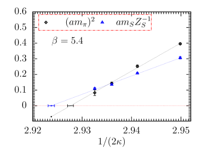
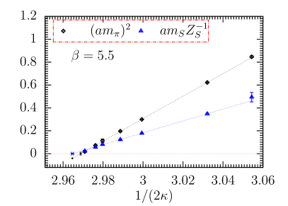
Figure 1: The subtracted gluino mass $am_{S}Z_{S}^{-1}$ and the squared adjoint pion mass $(am_{\text{a--}\pi})^{2}$ as a function of $1/(2\kappa)$, and the corresponding extrapolations towards the chiral point ($\kappa_{c}$) for two values of $\beta$.

In the case of lattice QCD, Wilson chiral perturbation theory to leading order shows a shift linear in $a$ in the dependence of the squared pion mass on the quark mass:

$$m_{\pi,\text{LO}}^{2}=2B_{0}m_{q}+2W_{0}a\,,$$ (24)

with certain low-energy constants $B_{0}$ and $W_{0}$ [15, 16]. On the other hand, for the PCAC quark mass, defined by means of the chiral Ward identity, exactly the same shift is present in leading order [17],

$$2B_{0}m_{\text{PCAC,LO}}=2B_{0}m_{q}+2W_{0}a\,.$$ (25)

Consequently, at vanishing pion mass, the remnant $m_{\text{PCAC}}$ is of order $a^{2}$, and this result is not changed in higher orders of chiral perturbation theory,

$$m_{\text{PCAC}}=O(a^{2})\quad\text{at}\quad m_{\pi}^{2}=0.$$ (26)

In SYM the adjoint pion mass can be calculated in partially quenched chiral perturbation theory [14]. We haven’t evaluated the contributions from the lattice terms explicitly, but the structure of terms is similar to those for QCD, and therefore we expect that in SYM the remnant gluino mass $\Delta m_{S}$ at vanishing adjoint pion mass is of order $a^{2}$, too. In order to check this numerically, the masses have to be expressed in a physical scale. We use the scale $w_{0}$, defined through the gradient flow; for details see [11]. In Fig. 2 we show the remnant gluino mass as a function of the squared lattice spacing $a^{2}$. The line through the points extrapolates to zero within errors. For an analogous plot linear in $a$ this is by far not the case. Having only two points available, one has to be cautious drawing conclusions, but the result clearly indicates that the remnant gluino mass $\Delta m_{S}$ vanishes proportional to $a^{2}$ in the continuum limit.

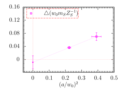
Figure 2: The remnant gluino mass $\Delta(w_{0}m_{S}Z_{S}^{-1})$ at vanishing $m_{\text{a--}\pi}^{2}$ as a function of the lattice spacing squared. The common scale is set through the gradient flow parameter $w_{0}$.

5 Conclusions

We have presented a method for the numerical analysis of SUSY Ward identities in supersymmetric Yang-Mills theory on a lattice, which employs the expectation values of the relevant operators on a range of time slices. The statistical correlations between all observables are taken into account by means of a generalised least squares procedure. Applied to SUSY Yang-Mills theory with gauge group SU(3), the value of the hopping parameter, where the renormalised gluino mass vanishes, can be estimated, and is in rough agreement with the estimation using the adjoint pion mass. The difference between the estimates appears to vanish in the continuum limit. Our results represent the first continuum extrapolation of SUSY Ward identities. The scaling of lattice artefacts as of $O(a^{2})$ is in agreement with theoretical expectations.

References

- [1] M. Lüscher, S. Sint, R. Sommer and P. Weisz, Nucl. Phys. B 478 (1996) 365 [arXiv: hep-lat/9605038 ].
- [2] F. Farchioni, A. Feo, T. Galla, C. Gebert, R. Kirchner, I. Montvay, G. Münster and A. Vladikas, Eur. Phys. J. C 23 (2002) 719 [arXiv: hep-lat/0111008 ].
- [3] G. Bergner, JHEP 1001 (2010) 024 [arXiv: 0909.4791 [hep-lat]].
- [4] G. Bergner, P. Giudice, G. Münster, I. Montvay and S. Piemonte, JHEP 1603 (2016) 080 [arXiv: 1512.07014 [hep-lat]].
- [5] S. Ali, G. Bergner, H. Gerber, P. Giudice, I. Montvay, G. Münster and S. Piemonte, PoS(LATTICE2016) (2016) 222 [arXiv: 1610.10097 [hep-lat]].
- [6] B. de Wit and D. Z. Freedman, Phys. Rev. D 12 (1975) 2286.
- [7] G. Curci and G. Veneziano, Nucl. Phys. B 292 (1987) 555.
- [8] Y. Taniguchi, Phys. Rev. D 63 (2000) 014502 [arXiv: hep-lat/9906026 ].
- [9] S. Musberg, G. Münster and S. Piemonte, JHEP 1305 (2013) 143 [arXiv: 1304.5741 [hep-lat]].
- [10] S. L. Marshall, J. G. Blencoe, Am. J. Phys. 73 (2005) 69.
- [11] S. Ali, G. Bergner, H. Gerber, P. Giudice, G. Münster, I. Montvay, S. Piemonte and P. Scior, [arXiv: 1801.08062 [hep-lat]].
- [12] K. Demmouche, F. Farchioni, A. Ferling, I. Montvay, G. Münster, E. E. Scholz and J. Wuilloud, Eur. Phys. J. C 69 (2010) 147 [arXiv: 1003.2073 [hep-lat]].
- [13] G. Veneziano and S. Yankielowicz, Phys. Lett. B 113 (1982) 231.
- [14] G. Münster and H. Stüwe, JHEP 1405 (2014) 034 [arXiv: 1402.6616 [hep-th]].
- [15] S. R. Sharpe and R. L. Singleton, Jr, Phys. Rev. D 58 (1998) 074501 [arXiv: hep-lat/9804028 ].
- [16] G. Rupak and N. Shoresh, Phys. Rev. D 66 (2002) 054503. [arXiv: hep-lat/0201019 ].
- [17] S. R. Sharpe and J. M. S. Wu, Phys. Rev. D 71 (2005) 074501 [arXiv: hep-lat/0411021 ].