The $s$-wave scattering length of a Gaussian potential

Abstract

We provide accurate expressions for the $s$-wave scattering length for a Gaussian potential well in one, two and three spatial dimensions. The Gaussian potential is widely used as a pseudopotential in the theoretical description of ultracold atomic gases, where the $s$-wave scattering length is a physically relevant parameter. We first describe a numerical procedure to compute the value of the $s$-wave scattering length from the parameters of the Gaussian but find that its accuracy is limited in the vicinity of singularities that result from the formation of new bound states. We then derive simple analytical expressions that capture the correct asymptotic behavior of the $s$-wave scattering length near the bound states. Expressions that are increasingly accurate in wide parameter regimes are found by a hierarchy of approximations that capture an increasing number of bound states. The small number of numerical coefficients that enter these expressions is determined from accurate numerical calculations. The approximate formulas combine the advantages of the numerical and approximate expressions, yielding an accurate and simple description from the weakly to the strongly interacting limit.

I Introduction

The interest in the accurate determination of $s$-wave scattering length has increased in recent decades due to its importance in the description of systems of ultracold atoms Pethick and Smith (2002); Pitaevskii and Stringari (2016). As the range of the interparticle interactions is usually much smaller than the average inter-particle distances, the effects of interactions can be expressed in terms of the scattering amplitude between pairs of particles. For dilute gases at ultracold temperatures, the kinetic energies are low and, therefore, the main contribution to the amplitude comes from the $s$-wave scattering at zero momentum. Particle interactions are thus determined completely by a single parameter: the $s$-wave scattering length Roger G. Newton (1982); Pethick and Smith (2002). In theoretical calculations, it is therefore not necessary to consider the detailed interaction potential between the particles. Instead, a pseudopotential may be chosen in a way to reproduce the desired value of the $s$-wave scattering length, which can simplify the required computations considerably Pethick and Smith (2002).

One of the simplest and most popular pseudopotentials is the Dirac $\delta$ potential. Its straightforward application is, however, restricted to one dimension, since in two or three dimensions it is meaningless without renormalization Esry and Greene (1999); Rontani et al. (2017); Doganov et al. (2013). An alternative option is to use finite-range pseudopotentials, e.g. the finite square well von Stecher et al. (2008); Blume (2012), Troullier-Martins Bugnion et al. (2014); Whitehead et al. (2016), Pöschl-Teller Forbes et al. (2011); Galea et al. (2016), or Gaussian potential von Stecher et al. (2008); Blume (2012); Doganov et al. (2013); Christensson et al. (2009); Klaiman et al. (2014); Beinke et al. (2015); Imran and Ahsan (2015); Bolsinger et al. (2017a, b). The scattering length is finite for these pseudopotentials, but an extrapolation to zero range might be necessary to avoid an unphysical shape dependence von Stecher et al. (2008); Blume (2012); Forbes et al. (2011). The relationship between the parameter(s) of the potential and the scattering length is not always trivial. Apart from some special cases Farrell and van Zyl ; Forbes et al. (2011), numerical techniques are required to determine this relation Landau and Lifshitz (1977); Verhaar et al. (1985); Galea et al. (2017).

For Gaussian potentials, no closed-form analytic expressions are available and, for this reason, numerical approaches have been applied  Christensson et al. (2009); Parish et al. (2005); Johnson et al. (2012); Bolsinger et al. (2017a). In two dimensions, an approximate expression was derived by Doganov et al. Doganov et al. (2013). These authors considered two particles in a harmonic trap, where the Gaussian interparticle interaction is treated in a perturbative framework. The obtained second order correction combined with the analytical result of the contact pseudopotential  Busch et al. (1998); Farrell and van Zyl (2010) provides the approximate expression. Due to the perturbative approach, this approximation works quite well in the weakly interacting limit, but it deteriorates with increasing interaction strength.

In this paper, we derive approximate analytical expressions for the $s$-wave scattering length of a Gaussian pseudopotential in one, two and three dimensions. These expressions qualitatively describe the singularities of the $s$-wave scattering length at the formation of the first bound state, which is problematic for purely numerical approaches. Analytical formulas for weak interactions are derived in one and two dimensions, where the $s$-wave scattering length has a singularity at zero interaction strength. In order to improve the accuracy, the approximate expressions are generalized by including the effects of additional bound states. The unknown parameters in this ansatz are determined by non-linear fitting to accurate numerical results. The obtained formulas are robust and simple and accurately provide the values for the $s$-wave scattering length in a wide regime of attractive interaction.

We describe and carefully benchmark a numerical method to accurately determine the scattering length of a short-range scattering potential in one, two, and three spatial dimensions. The approach is based on previous work of Verhaar Verhaar et al. (1985) and may be useful in its own right as it is able to provide very accurate results except for the immediate vicinity of the singularities. The numerical approach is applicable for general short-range potentials and is not restricted to potentials of Gaussian shape.

This paper is organized as follows: In Sec. II, after stating the problem and discussing the required asymptotic conditions for scattering wave functions, we present an accurate numerical approach for determining the $s$-wave scattering length along with benchmark calculations for a Gaussian potential. In Sec. III approximate analytic expressions for the $s$-wave scattering length of a Gaussian potential are derived before more accurate, generalized expressions with numerically determined parameters are introduced. Three appendices provide additional details on derivations and numerical issues with determining the position of singularities in the scattering length, respectively.

II Numerical determination of the $S$-wave scattering length

II.1 Solution of the two-body problem and connection with the $s$-wave scattering length

II.1.1 Two-body scattering problem

Let us consider a two-particle scattering process with the following $n$-dimensional Hamiltonian:

$$H_{2p} = -\frac{\hbar^{2}}{2m_{1}}\nabla^{2}_{1}-\frac{\hbar^{2}}{2m_{2}}\nabla^{2}_{2}+V(|{\mathbf{r}}_{1}-{\mathbf{r}}_{2}|)\ ,$$ (1)

where $V(|{\mathbf{r}}_{1}-{\mathbf{r}}_{2}|)$ is a spherically symmetric particle-particle interaction potential, and $m_{i}$, ${\mathbf{r}}_{i}$, and $\nabla^{2}_{i}$ are the mass, coordinate, and Laplace operator of the $i$th particle, respectively. Although our main target is the Gaussian potential, here we consider more general classes of potentials for which the numerical procedures can be applied. Specifically, we assume that the interaction is sufficiently short ranged to justify the existence of the scattering length. This is fulfilled in $n$ dimensions if $V(r)$ obeys the condition Case (1950); Frank et al. (1971)

$$\int\limits_{A}^{\infty}|V(r)|r^{n-1}\mbox{d}r<\infty$$

for a finite $A$. It is sufficient to assume that the potential decreases faster than $1/r^{n+\varepsilon}$ with $\varepsilon>0$ at sufficiently large distance. In addition, we suppose that the potential is regular at the origin or diverges, at most, with $1/r^{s}$ with $s<1$. This condition is necessary to uniquely define the appropriate boundary conditions at the origin for the purpose of the numerical procedure. The $s$-wave scattering length can still be defined for more strongly divergent potentials Frank et al. (1971); Andrews (1976), but the numerical procedure would have to be modified in this case.

The eigenproblem for the Hamiltonian (1) can be simplified by introducing the center of mass coordinate, ${\mathbf{R}}=(m_{1}{\mathbf{r}}_{1}+m_{2}{\mathbf{r}}_{2})/(m_{1}+m_{2})$, and relative coordinate, ${\mathbf{r}}={\mathbf{r}}_{1}-{\mathbf{r}}_{2}$. Then the wave function can be separated as  Roger G. Newton (1982)

$$\Psi_{nD}^{2p}({\bf r}_{1},{\bf r}_{2})=\exp(i{\bf Q}\cdot{\bf R}/\hbar)\,\psi_{nD}({\bf r})\ ,$$

where ${\bf Q}$ is the total momentum of the two particles. The relative wave function $\psi_{nD}({\bf r})$ is an eigenfunction of the Hamiltonian of the relative motion,

$$H\,\Psi_{nD}({\bf r}) = E\,\Psi_{nD}({\bf r})\$$ (2)

with

$$H=-\frac{\hbar^{2}}{2\mu}\nabla^{2}+V(r)\ ,$$ (3)

where $E$ is the scattering energy and $\mu=m_{1}m_{2}/(m_{1}+m_{2})$ is the reduced mass.

II.1.2 The $s$-wave scattering and boundary conditions

Due to the spherical symmetry of the potential, Eq. (2) can be further simplified by solving the angular-coordinate-dependent part separately through eigenstates of the angular momentum operator. By definition, $s$-wave scattering correspond to zero angular momentum with a radially symmetric wave function. The radial coordinate dependence in Eq. (2) can be obtained from the following differential equation for the general $n$-dimensional case  Verhaar et al. (1985); uto :

$$-\frac{\hbar^{2}}{2\mu}\left(\frac{\mbox{d}^{2}}{\mbox{d}r^{2}}+\frac{n-1}{r}\frac{\mbox{d}}{\mbox{d}r}\right)\Phi_{nD}(r) +$$ (4)

$$+\left(V(r)-E\right)\Phi_{nD} (r)=0\ ,$$

where $\Phi_{nD}(r)$ is the radial part of the relative wave function $\psi^{rel}_{nD}({\bf r})$. For ultracold atoms, only low-energy scattering processes are relevant and we may set $E=0$. As we see in the following section, it also provides us with a simple way to define the $s$-wave scattering length. Appropriate boundary conditions for the differential equation (4) can be obtained from smoothness and symmetry considerations in the limit $r\rightarrow 0$ (see the detailed description in Appendix A), as

$$\Phi_{nD}(0)=1\ , \Phi_{nD}^{\prime}(0)=0\ .$$ and (5)

II.1.3 Scattering length

For a short-range potential, the asymptotic of the wave function $\Phi_{nD}(r)$ at distances much larger than the characteristic length scale of the potential $\ell_{v}$ is given by a solution of Eq. (4) with $V(r)=0$ and $E=0$, which is a linear combination of a constant and $r$ in one dimension (1D), $\mbox{ln}\left(r\right)$ in 2D, and $1/r$ in 3D. The $s$-wave scattering length is defined by the ratio of the corresponding constants in this linear combination Verhaar et al. (1985); uto ,

$$\mbox{if }r\gg\ell_{v}\begin{cases}\Phi_{1D}(r)\approx{\mathcal{N}}_{1D}\left(r-a^{1D}_{s}\right)\ ,\\ \Phi_{2D}(r)\approx{\mathcal{N}}_{2D}\left[\mbox{ln}\left(\frac{2r}{a^{2D}_{s}}\right)-\gamma\right]\ ,\\ \Phi_{3D}(r)\approx{\mathcal{N}}_{3D}\left(1-\frac{a^{3D}_{s}}{r}\right)\ .\end{cases}$$ (6)

Here $a^{nD}_{s}$ is the $n$-dimensional $s$-wave scattering length, $\gamma=0.5772\ldots$ is the Euler-Mascheroni constant, and $\mathcal{N}_{nD}$ is a scalar factor. The scattering length can be expressed as a limit of the function $\Phi_{nD}(r)$ and its first derivative by eliminating the unknown parameter $\mathcal{N}_{nD}$ Verhaar et al. (1985); a2d ; uto as

$$a^{1D}_{s} = \lim_{r\rightarrow\infty}\left(r-\frac{\Phi_{1D}(r)}{\Phi_{1D}^{\prime}(r)}\right)\ ,$$ (7)

$$a^{2D}_{s} = \lim_{r\rightarrow\infty}2r\exp{\left(-\frac{\Phi_{2D}(r)}{r\Phi_{2D}^{\prime}(r)}-\gamma\right)}\ ,$$ (8)

$$a^{3D}_{s} = \lim_{r\rightarrow\infty}\left(r-\frac{r\Phi_{3D}(r)}{r\Phi_{3D}^{\prime}(r)+\Phi_{3D}(r)}\right)\ .$$ (9)

As can be seen from the expressions above, $a^{2D}_{s}$ is always positive by definition, while $a^{1D}_{s}$ and $a^{3D}_{s}$ can be of either sign. In the limiting case where the scattering potential is absent the solution of Eq. (4) becomes a zero-energy plane wave, i.e. the constant 1. Therefore, we have $a^{1D}_{s}\to\infty$ and $a^{2D}_{s}\to\infty$, while $a^{3D}_{s}\to 0$. This means that the scattering length develops a singularity when $V(r)\to 0$ in one and two dimensions.

II.2 One and three dimensions

The radial Schrödinger equation can be simplified by introducing the functions Verhaar et al. (1985)

$$u_{3D}(r) =r\,\Phi_{3D}(r)\quad\textrm{and}$$ (10)

$$u_{1D}(r) =\Phi_{1D}(r).$$ (11)

Substituting Eq. (10) into the radial Schrödinger equation (4) and the expression for the $s$-wave scattering length (9), we obtain identical equations for three and one dimensions,

$$\left(-\frac{\hbar^{2}}{2\mu}\frac{\mbox{d}^{2}}{\mbox{d}r^{2}}+V(r)-E\right)u_{1D/3D}(r)=0\ ,$$ (12)

$$a^{1D/3D}_{s}=\lim_{r\rightarrow\infty}\left(r-\frac{u_{1D/3D}(r)}{u_{1D/3D}^{\prime}(r)}\right)\ .$$ (13)

The boundary conditions are obtained by substituting Eq. (10) into Eq. (5) and now differ between one and three dimensions,

$$u_{1D}(0)=1\ , u_{1D}^{\prime}(0)=0\ ,$$ (14)

$$u_{3D}(0)=0\ , u_{3D}^{\prime}(0)=1\ .$$ (15)

In a numerical procedure, we may assume that the functions $u_{1D/3D}(r)$ and $u_{1D/3D}^{\prime}(r)$ can only be given with limited numerical accuracy ($p$) as

$$u_{1D/3D}(r) = \lim\limits_{p\rightarrow\infty}\tilde{u}_{1D/3D}(r;p)\ ,$$

$$u_{1D/3D}^{\prime}(r) = \lim\limits_{p\rightarrow\infty}\tilde{u}_{1D/3D}^{\prime}(r;p)\ ,$$

where $p$ relates to the accuracy of the decimal representation and the numerical method itself. For the numerical determination of the scattering length, one should then consider the combined limit,

$$a^{1D/3D}_{s} = \lim_{r,p\rightarrow\infty}\underbrace{\left(r-\frac{\tilde{u}_{1D/3D}(r;p)}{\tilde{u}_{1D/3D}^{\prime}(r;p)}\right)}_{\tilde{a}_{s}^{1D/3D}(r;p)}\ .$$

II.3 Two-dimensional case

In two dimensions, the original radial function $\Phi_{2D}(r)$ is used directly. Here a numerical instability is present as a result of the $1/r$ singularity in the first derivative term of the radial Schrödinger equation (4) for two dimensions. The instability can be avoided by giving the boundary conditions at distance $r=\epsilon$, where $\epsilon$ is chosen large enough to avoid the numerical difficulties but small enough to approximately satisfy the conditions of Eq. (5)

$$\Phi_{2D}(\epsilon)\approx 1\ ,\hskip 56.9055pt\Phi^{\prime}_{2D}(\epsilon)\approx 0\ .$$ (16)

Consequently, $\epsilon$ becomes another parameter of the numerical evaluation besides the numerical accuracy ($p$). The scattering length is then obtained from the composite limit

$$a_{s}^{2D} = \lim_{\stackrel{{\scriptstyle r,p\rightarrow\infty}}{{\epsilon\rightarrow 0}}}\underbrace{2r\exp{\left(-\frac{\tilde{\Phi}_{2D}(r;\epsilon,p)}{r\tilde{\Phi}_{2D}^{\prime}(r;\epsilon,p)}-\gamma\right)}}_{\tilde{a}_{s}^{2D}(r;\epsilon,p)}\ ,$$ (17)

where $\tilde{\Phi}_{2D}(r;\epsilon,p)$ represents the approximate numerical solution of Eqs. (4) and (16) with

$$\Phi_{2D}(r) = \lim\limits_{\stackrel{{\scriptstyle p\rightarrow\infty}}{{\epsilon\rightarrow 0}}}\tilde{\Phi}_{2D}(r;\epsilon,p)\ .$$ (18)

II.4 The Gaussian potential and the convergence of numerical results

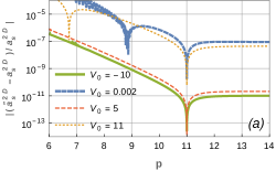
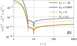
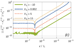
Figure 1: Relative error in the two-dimensional $s$-wave scattering length compared to a reference value $a_{s}^{2D}$ computed with parameters $p=11$, $r=10L$, $\epsilon=10^{-6}L$. Shown is the parameter dependence (a) on the numerical precision $p$, (b) on the cutoff distance $r$, and (c) on the boundary parameter $\epsilon$ for different values of the potential strength $V_{0}$.

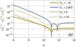
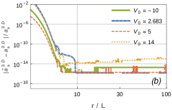
Figure 2: Relative error in the three-dimensional $s$-wave scattering length compared to a reference value $a_{s}^{3D}$ computed with parameters $p=11$, $r=10L$. Shown is the parameter dependence (a) on the numerical precision $p$ and (b) on the cutoff distance $r$ for different values of the potential strength $V_{0}$.

We now apply this approach to the Gaussian potential

$$V(r)=-\frac{V_{0}}{2L^{2}}e^{-\frac{r^{2}}{L^{2}}}\ ,$$ (19)

which depends on parameters for the potential strength $V_{0}$ and the length scale $L$. Since we are free to use $L$ as a scale parameter, we find that the ratio $a_{s}/L$ depends only on the single dimensionless parameter $V_{0}\mu/\hbar^{2}$. The results of the numerical calculations and their physical interpretation will be discussed in Sec. III along with analytic approximations. Here we discuss the details and convergence properties of the numerical approach.

The numerical calculations are performed with the fourth-order Runge-Kutta method of the Mathematica program package  Wolfram Research, Inc. (2014). The parameter $p$ is considered here as a composite variable. We set the parameters ”AccuracyGoal” and ”PrecisionGoal”, which quantify the accuracy and precision of the numerical method, respectively, to the same number $p$. The ”WorkingPrecision”, which controls the number of the digits in the calculations, is set to $p+5$. Ideally, we should consider the infinite limit of $p$ and $r$, and the zero limit of $\epsilon$. On the computer this limit is considered numerically with a finite accuracy. The convergence properties of the numerical procedure can be seen from Figs. 1 and 2 for the $s$-wave scattering length of the Gaussian potential in two and three dimensions, respectively. We first compute a fairly accurate reference value with a fixed choice of the accuracy parameters and then plot the relative error of the scattering length compared to the reference value as a function of the accuracy parameters.

In all cases, the relative error decays exponentially until the reference value of the accuracy parameter is reached. At that point, due to the equality of $\tilde{a}_{s}^{nD}=a_{s}^{nD}$, the curves abruptly drop to zero. Beyond that point, the relative error saturates to a constant value that corresponds to the numerical error of the reference value of the scattering length. In two dimensions (Fig. 1), the largest errors occur at $V_{0}=0.002\hbar^{2}/\mu$ and $V_{0}=11\hbar^{2}/\mu$, close to divergences of the scattering length (see Fig. 5). This demonstrates how the numerical accuracy is limited near the divergences of the scattering length.

In three dimensions, the $s$-wave scattering length diverges near to $V_{0}=2.683\hbar^{2}/\mu$, where the largest errors in are seen in Fig. 2(a). In the same graph, the case of $V_{0}=14\hbar^{2}/\mu$ has the second largest numerical error. In that case the scattering length is close to the zero crossing ($a_{s}^{3D}\approx 0.05L$). It is difficult to compute it accurately from Eq. (13) where a difference of small numbers [cutoff distance and inverse logarithmic derivative of $\Phi_{3D}(r)$] needs to be taken. This effect is even more notable as a function of the cutoff distance in Fig. 2(b), where the error in the case of $V_{0}=14\hbar^{2}/\mu$ is at least one order larger at larger distances compared to other values of the potential strength. Numerical rounding errors also explain the jumps in the cases of $V_{0}=-10\hbar^{2}/\mu$ and $V_{0}=5\hbar^{2}/\mu$, which are the limit of the chosen accuracy.

III Approximate expressions for Gaussian potential

III.1 Three-dimensional case

As can be seen in the previous section, the numerical approach is accurate in most cases, but fails near the divergences of the scattering length. Here we derive analytic approximations that can handle these numerically unstable regions. An alternative derivation based on the Lippmann-Schwinger equation is given in Appendix C.

In order to derive suitable approximations, we can make use of the fact that the Gaussian potential decays rapidly to zero with increasing distance. Contributions of the long-range part of the wave function, therefore, become negligible when they are multiplied by this potential compared to the other parts of the Schrödinger equation, e.g., Eq. (12). Let us specifically consider the simplest case of a shallow Gaussian potential in three dimensions that has no bound states. Thus the zero-energy wave function $u_{3D}(r)$ will be nodeless and can be safely approximated with the leading term of its Taylor expansion around $r=0$ in the product with the Gaussian potential as

$$e^{-\frac{r^{2}}{L^{2}}}\,u_{3D}(r) \approx e^{-\frac{r^{2}}{L^{2}}}\,r\ .$$ (20)

Note that the long-range asymptotics of $u_{3D}(r)$ that define the scattering length are (approximately) unaffected by this procedure. Substituting into Eq. (12) at $E_{rel}=0$, we obtain the differential equation

$$-\frac{\hbar^{2}}{2\mu}\frac{\mbox{d}^{2}}{\mbox{d}r^{2}}\bar{u}_{3D}(r)-\frac{V_{0}}{2L^{2}}e^{-\frac{r^{2}}{L^{2}}}r=0\ .$$ (21)

The function $\bar{u}_{3D}(r)$ can be obtained by integrating Eq. (21) twice,

$$\bar{u}_{3D}(r) = c_{1}^{3D}+c_{2}^{3D}r+\frac{\sqrt{\pi}V_{0}\mu}{4\hbar^{2}}\mbox{erf}\left(\frac{r}{L}\right)\ ,$$ (22)

where $\mathrm{erf}(x)=(2/\sqrt{\pi})\int_{0}^{x}\exp(-t^{2})dt$ is the error function. The coefficients in Eq. (22) can be determined by considering the boundary conditions (15) as

$$c_{1}^{3D}=0\ , c_{2}^{3D}=\frac{2-\frac{V_{0}\mu}{\hbar^{2}}}{2L}\ .$$

Examining these wave functions in the limit when $r$ goes to infinity and using the fact that $\lim_{r\rightarrow\infty}\mbox{erf}\left(\frac{r}{L}\right)=1$, if $L$ is finite, we obtained the following asymptotic expression:

$$\bar{u}_{3D}(r)\approx\frac{2-\frac{V_{0}\mu}{\hbar^{2}}}{2}\left(\frac{r}{L}-\frac{\sqrt{\pi}}{2}\frac{V_{0}}{V_{0}-\frac{2\hbar^{2}}{\mu}}\right)\ ,\ r\rightarrow\infty\ .$$ (23)

Substituting Eq. (23) into Eq. (13), the approximate relations between the $s$-wave scattering length and the parameters of the potential can be found as

$$\frac{\bar{a}_{s}^{3D}}{L} = \frac{\sqrt{\pi}}{2}\frac{V_{0}}{V_{0}-\frac{2\hbar^{2}}{\mu}}\ .$$ (24)

This approximate formula has a pole near the value of $V_{0}$ where the Gaussian potential well acquires the first bound state. The appearance of a pole, even though we had started out with assuming a nodeless wave function, validates the procedure but also signals a limit of validity of the approximation. On closer inspection, we find that the expression (24) describes the scattering length near the singularity qualitatively correctly, but the position of the pole is inaccurate. As can be seen in Fig. 3, further singularities appear when the potential well becomes deeper and these correspond to additional bound states. Although the approximation (24) includes only the first singularity, it can be sufficient for the use as a pseudopotential for ultracold atoms if only the qualitative behavior of the scattering length in the presence of up to one bound state is of interest.

In order to reproduce the behavior of the scattering length across a larger range of potential strengths, we generalize Eq. (24) by explicitly introducing a variable number of singularities in the following way:

$$\frac{a_{s}^{3D}}{L} \approx \sum_{i=1}^{n}\alpha_{i}\frac{V_{0}}{\left(V_{0}-W_{i}\right)}\ .$$ (25)

Here, $W_{i}$ and $\alpha_{i}$ are numerically determined parameters. The parameters $W_{i}$ are set to the values of $V_{0}$ where the numerically determined scattering length diverges (and changes sign). At these values of $V_{0}$ weakly bound states appear (see, e.g., Ref. Flügge (1999), problem 90). To achieve a high accuracy for approximations of the $s$-wave scattering length, it is important to use accurate values for these parameters (see the detailed description in Appendix B). The parameters $\alpha_{i}$ are obtained by nonlinear fitting of the approximate expression Eq. (25) to the numerically obtained scattering length. The fitting procedure is performed on the intervals $V_{0}\mu/\hbar^{2}\in[0,2.68]\cup[2.69,14]$ in order to avoid the singularities. The values of the fitted parameters are shown in Table 1. As can be seen in Fig. 3, including even one additional singularity in the model greatly improves Eq. (24) and qualitatively describes the fitted region. Each additional fitting parameter further improves the relative accuracy by more than one order of magnitude. In addition, the approximate formulas also dramatically improve the approximation of $a_{s}^{3D}$ outside the fitted regime with each fitting parameter.

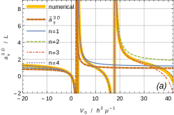
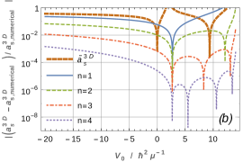
Figure 3: (a) Three-dimensional $s$-wave scattering length from the numerical and the approximate expression. (b) The difference between the approximative and numerical scattering length values. The parameters of the numerical simulations are set to $p=11$ and $r=10L$. The values of the parameters for the approximative expressions can be found in Table 1.

n	$W_{n}\left(\hbar^{2}/\mu\right)$	$\alpha_{1}$	$\alpha_{2}$	$\alpha_{3}$	$\alpha_{4}$
1	2.68400465092	1.11942413969
2	17.7956995472	1.12031910105	0.378402820446
3	45.5734799205	1.12034867267	0.322141242778	0.332600792963
4	85.9634003809	1.12034897387	0.326461774698	0.135560767226	0.375312300726
$\tilde{a}_{s}^{3D}$	2	$\sqrt{\pi}/2\approx$ 0.8862269

Table 1: Numerical values of parameters for the three-dimensional approximate expression (25).

III.2 One-dimensional case

We follow an analogous procedure to the three-dimensional case by approximately solving the Schrödinger equation for large $r$. Although the form of the one-dimensional Schrödringer equation is equivalent to the three-dimensional one [Eq. (12)], the boundary conditions of Eqs. (14) and (15) differ. This has the consequence that the zeroth-order term in the Taylor expansion of $u_{1D}(r)$ does not vanish and thus we may approximate the differential equation as

$$-\frac{\hbar^{2}}{2\mu}\frac{\mbox{d}^{2}}{\mbox{d}r^{2}}\bar{u}_{1D}(r)-\frac{V_{0}}{2L^{2}}e^{-\frac{r^{2}}{L^{2}}}=0\ .$$ (26)

Equation (26) can be solved and provides the following approximate expression for the wave function and the $s$-wave scattering length:

$$\bar{u}_{1D}(r) = 1-\frac{V_{0}\mu}{2\hbar^{2}}\left[e^{-\frac{r^{2}}{L^{2}}}+\sqrt{\pi}\mbox{erf}\left(\frac{r}{L}\right)\frac{r}{L}-1\right]\ ,$$ (27)

$$\frac{\bar{a}_{s}^{1D}}{L} = \ \frac{1}{\sqrt{\pi}}+\frac{2}{\sqrt{\pi}}\frac{\hbar^{2}}{V_{0}\mu}.$$ (28)

Comparing the obtained expression (28) with the three-dimensional result (24), it can be seen that the first singularity in one dimension is located in the origin, while in three dimensions it is displaced to a finite value of attractive potential strength. As every singularity indicates the creation of a new bound state, the former statement is related to a well-known property: in one dimension, there is always a bound state at any nonzero attractive potential, meanwhile, in three dimensions, the bound state appears at some finite potential strength.

The approximate expression (28) can be further improved if we expand the function $u_{1D}(r)$ in a Taylor series around the origin. As we are interested in the behavior of the singularity in the origin, we can consider the limit of $V_{0}$ approaching zero, where the coefficients of the Taylor expansion can be determined (see the detailed description in Appendix D). By examining the asymptotic properties of the wave function we obtain the following approximate formula for the scattering length:

$$\frac{\bar{\bar{a}}_{s}^{1D}}{L} = \sqrt{\frac{2}{\pi}}+\frac{2}{\sqrt{\pi}}\frac{\hbar^{2}}{V_{0}\mu},$$ (29)

which differs from Eq. (28) only in the constant offset. This expression fits better with the numerically obtained results, but it is still inaccurate at larger absolute values of the potential strength. In analogy to the three dimensional case [Eq. (25)], the accuracy of Eq. (29) can be further improved by including additional singularities,

$$\frac{a_{s}^{1D}}{L} \approx \sqrt{\frac{2}{\pi}}+\frac{2}{\sqrt{\pi}}\frac{\hbar^{2}}{V_{0}\mu}+\sum_{i=1}^{n}\alpha_{i}\frac{V_{0}}{(V_{0}-W_{i})}\ ,$$ (30)

where the parameters $W_{i}$ are obtained directly from the numerical solution of the differential equation. The parameter values $\alpha_{i}$ are obtained nonlinearly fitting the expression (30) to the numerical data in the interval $V_{0}\hbar^{2}/\mu\in[1.0,8.0]$.

A comparison of the approximate and the numerical results is shown in Fig. 4. Similarly to the three-dimensional case, the relative error from the numerical solution gradually decreases with the number of the parameter pairs.

n	$W_{n}\left(\hbar^{2}/\mu\right)$	$\alpha_{1}$	$\alpha_{2}$	$\alpha_{3}$	$\alpha_{4}$
1	8.6490975	0.52689372
2	30.106280	0.51419392	0.35899733
3	64.193333	0.51460375	0.20675606	0.36766012
4	110.88204	0.51459468	0.24033314	0.040512694	0.44420188

Table 2: Numerically determined parameters for the one-dimensional approximate expression in Eq. (36).

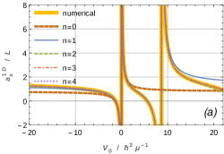
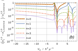
Figure 4: (a) One-dimensional $s$-wave scattering length from the numerical and the approximate expression. (b) The difference between the approximate and numerical values of the scattering length. The parameters of the numerical simulations are set to $p=11$, $r=10L$. The parameter values for the approximate expressions are tabulated in Table 2. The $n=0$ approximation corresponds to Eq. (29).

III.3 Two-dimensional case

In two dimensions the function $\Phi_{2D}(r)$ is considered, where the corresponding Schrödinger equation (4) at $E_{rel}=0$ and boundary conditions (5) provide the following approximate differential equation:

$$-\frac{\hbar^{2}}{2\mu}\left(\frac{\mbox{d}^{2}}{\mbox{d}r^{2}}+\frac{1}{r}\frac{\mbox{d}}{\mbox{d}r}\right) \bar{\Phi}_{2D}(r)+V(r)=0\ .$$ (31)

Solving Eq. (31), the radial function can be obtained as

$$\bar{\Phi}_{2D}(r) = 1+\frac{V_{0}}{4}\left[\mbox{Ei}\left(-r^{2}\right)-\gamma-2\,\mbox{ln}(r)\right]\ ,$$ (32)

where Ei$(x)=-\int_{-x}^{\infty}\frac{e^{-t}}{t}\mbox{d}t$ is the exponential integral function. At large particle separation, the exponential integral function goes to zero, $\lim_{r\rightarrow\infty}\mbox{Ei}\left(-r^{2}\right)=0$, and therefore Eq. (64) can be approximated with the following expression:

$$\bar{\Phi}_{2D}(r) \approx 1-\frac{V_{0}\mu}{4\hbar^{2}}\left[\gamma+2\,\mbox{ln}\left(\frac{r}{L}\right)\right]\ ,\hskip 14.22636ptr\rightarrow\infty\ .$$ (33)

Using this asymptotic formula, the approximate expression of the $s$-wave scattering length can be determined from Eq. (8) as

$$\frac{\bar{a}_{s}^{2D}}{L} = 2e^{\frac{-3\gamma}{2}+\frac{2\hbar^{2}}{V_{0}\mu}}\ .$$ (34)

A singularity appears again in the origin, like in the one-dimensional case, as a consequence of the fact that any arbitrarily weak Gaussian potential well in two dimensions has at least one bound state. In analogy to the procedure of Appendix D, in one dimension, we can thus determine an improved prefactor to arrive at the approximation

$$\frac{\bar{\bar{a}}_{s}^{2D}}{L} = \sqrt{8}e^{\frac{-3\gamma}{2}+\frac{2\hbar^{2}}{V_{0}\mu}}\ .$$ (35)

This approximate formula (35) is equivalent to the previously mentioned formula of Doganov $et$ al. Doganov et al. (2013), where Eq. (35) was derived in a different manner using perturbation theory. This expression is not very accurate at larger values of potential strength and can be improved by including additional singularities in the same manner as done previously to obtain

$$\frac{a_{s}^{2D}}{L} \approx \sqrt{8}e^{-\frac{3\gamma}{2}+\frac{2\hbar^{2}}{V_{0}\mu}+\sum\limits_{i=1}^{n}\alpha_{i}\frac{V_{0}}{(V_{0}-W_{i})}}\ .$$ (36)

We determined the parameters $W_{i}$ with the numerical differential equation solver and fitted the parameters $\alpha_{i}$ on the interval $V_{0}\in[1,10]\hbar^{2}/\mu$.

The numerical and approximate values for the two-dimensional $s$-wave scattering length are shown in Fig. 5. In contrast to the one- and three-dimensional results, the two-dimensional scattering length is always positive and single poles occur not in the scattering length itself but in its logarithm. Similarly to the previous cases, increasing the number of fitted parameter pairs successively improves the approximate values for the scattering length inside and outside the fitted region.

n	$W_{n}\left(\hbar^{2}/\mu\right)$	$\alpha_{1}$	$\alpha_{2}$	$\alpha_{3}$	$\alpha_{4}$
1	11.076903	0.33553384
2	35.081301	0.30476380	0.20423041
3	71.774188	0.30609585	0.10986740	0.19295017
4	121.10485	0.30605919	0.13171195	0.017845686	0.22077743

Table 3: Numerically determined parameters for the two-dimensional approximate expression in Eq. (36).

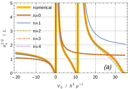
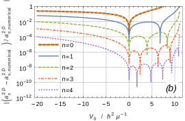
Figure 5: (a) Two-dimensional $s$-wave scattering length from the numerical and the approximate expression. (b) The difference between the approximative and numerical scattering length values. The parameters of the numerical simulations are set to the following: $p=11$, $r=10L$, and $\epsilon=10^{-6}L$. The values of the parameters for the approximative expressions can be found in Table 3. The $n=0$ approximations correspond to Eq. (35).

IV Conclusion

We have introduced approximate expressions for the $s$-wave scattering length for a Gaussian potential in one, two, and three dimensions. These may be useful on their own or can improve the accuracy of a numerical determination of the scattering length by providing the correct asymptotic behavior near singularities. The lowest-level expressions can be obtained as simple parameter-free approximations derived from the two-particle Schrödinger equation. They can qualitatively describe the singularity at the first bound-state formation, where numerical methods usually fail or provide inaccurate answers. In one and two dimensions these expressions can be further improved analytically by examining the weakly interacting limit, where the leading terms can be given exactly. More accurate expressions generalize the simple formulas in a straightforward way by including additional singularities, where the unknown parameters are determined from accurate numerical computations. The obtained formulas improve the accuracy for the whole region of the potential strength. In three dimensions, where the singularity due to appearance of the first bound state appears at a finite value of the potential strength, the accuracy of this value crucially limits the obtainable accuracy for the $s$-wave scattering length.

The Gaussian potential well has its main application for use as a pseudopotential in the description of ultracold atoms in the parameter regime between zero interaction and the first nontrivial bound state. In this region, the relative error of the parameterized approximate formulas reaches below $10^{-4}$ and thus they provide accurate, reliable, and simple formulas to connect the parameters of the Gaussian potential to the $s$-wave scattering length.

V Acknowledgement

We wish to acknowledge Jonas Cremon, Christian Forssén, and Stephanie Reimann for providing a note on the numerical determination of the $s$-wave scattering length and we thank Ali Alavi and Tal Levy for discussion and for initiating our interest in this problem. P.J. and J.B. thank the Max Planck Institute for Solid State Research for hospitality during an extended stay where this work was completed. This work was supported by the Marsden Fund of New Zealand (Contract No. MAU1604). A.Yu.Ch. acknowledges support from the JINR–IFIN-HH projects.

Appendix A Boundary conditions for the scattering problem

We consider a short-range interaction potential as specified in Sec. II.1.1 and extend a similar argument given in Ref. Perelomov and Zel’dovich (1998) (see also Cherny and Shanenko (2001) for the boundary conditions in two dimensions) to subleading order. To obtain the boundary conditions, let us multiply Eq. (4) by $r^{2}$ and consider the limit of $r\rightarrow 0$ as

$$\lim\limits_{r\rightarrow 0}{\Bigg{[}}-\frac{\hbar^{2}}{2\mu}\left(r^{2}\frac{\mbox{d}^{2}}{\mbox{d}r^{2}}+r(n-1)\frac{\mbox{d}}{\mbox{d}r}\right)\Phi_{nD}(r)\,+\hskip 14.22636pt$$ (37)

$$+r^{2}\left[V(r)-E\right]\Phi_{nD}(r){\Bigg{]}}=0\ .$$

The second term vanishes more quickly than the other ones in the limit of $r\rightarrow 0$ if the potential is nonsingular at the origin and diverges, at most, like $1/r^{s}$ with $s<2$. In order to obtain the leading term of the radial wave function, we may ignore this term and consider the differential equation

$$\lim\limits_{r\rightarrow 0}{\Bigg{[}}-\frac{\hbar^{2}}{2\mu}\left(r^{2}\frac{\mbox{d}^{2}}{\mbox{d}r^{2}}+r(n-1)\frac{\mbox{d}}{\mbox{d}r}\right)\Phi^{a}_{nD}(r){\Bigg{]}}=0\ ,$$ (38)

where $\Phi^{a}_{nD}(r)$ is asymptotic solution of $\Phi_{nD}(r)$ in the origin.

Let us first consider the cases of two and three dimensions. Here the origin is a singular point due to the $1/r$ term in Eq. (4). For Eq. (38), we find the explicit solutions

$$\Phi^{a}_{2D}(r) = d_{2D}\,\mbox{ln}(r)+c_{2D}\ ,$$ (39)

$$\Phi^{a}_{3D}(r) = \frac{d_{3D}}{r}+c_{3D}\ .$$ (40)

The parameters $d_{2D}$, $c_{2D}$, $d_{3D}$, and $c_{3D}$ are arbitrary constants. The functions $\mbox{ln}(r)$ and $1/r$ are singular at $r=0$, which would provide a nonsmooth wave function. Moreover, in the kinetic part of the Hamiltonian, the Laplacian operator would generate a Dirac $\delta$ contribution that is not compensated by the potential part in the Schrödinger equation Perelomov and Zel’dovich (1998). Hence, these irregular parts should be eliminated by setting the scalar factors $d_{2D}$ and $d_{3D}$ to 0. Setting the remaining coefficients $c_{nD,1}$ and $c_{nD,2}$ to 1, we obtain the boundary condition $\Phi(0)=0$, i.e., the first part of Eq. (5).

In one dimension the origin is a regular point of Eq. (4) and parity is a good quantum number. An explicit solution is

$$\Phi^{a}_{1D}(r)=d_{1D}{r}+c_{1D}\ .$$ (41)

Since $s$-wave scattering demands an even-parity solution, we set $d_{1D}=0$ and $c_{1D}=1$ to obtain the boundary conditions (5) in the one-dimensional case.

It remains to derive the correct boundary condition for the first derivative, $\Phi^{\prime}_{nD}(0)$. A separate consideration is necessary here, since the sub-leading term in the radial wave function may lead to a divergent derivative. We specifically consider the case $E=0$ but nonzero energies can be studied the same way. Let us integrate the Schrödinger equation in $n$ dimensions,

$$\nabla^{2}\Phi(x)=\frac{2\mu}{\hbar^{2}}V(x)\Phi(x)$$ (42)

over a small ball of radius $r$. For the left-hand side, one can apply Gauss’ theorem, which yields for a radially symmetric wave function,

$$\int_{|\vec{x}|\leqslant r}\nabla^{2}\Phi(x)\mbox{d}^{n}x=\oint_{|\vec{x}|=r}\mbox{d}\vec{S}\cdot\nabla\Phi(x)=S_{n}\Phi^{\prime}(r)r^{n-1},$$ (43)

where $S_{n}=2\pi^{n/2}/\Gamma(n/2)$ is the surface area of the sphere of the unit radius in $n$ dimensions, and $\Gamma(z)$ denotes the Gamma function. When $\Phi(0)=1$, the leading term on the right-hand side of (42) becomes $\frac{2\mu C}{\hbar^{2}}r^{-s}$, where $C$ is a constant. After integration, this term yields

$$\int_{|\vec{x}|\leqslant r}\frac{2\mu}{\hbar^{2}}V(x)\Phi(x)\mbox{d}^{n}x \simeq\int_{0}^{r}\frac{2\mu C}{\hbar^{2}}x^{-s}S_{n}x^{n-1}\mbox{d}x$$

$$\simeq S_{n}\frac{2\mu C}{\hbar^{2}}\frac{r^{n-s}}{n-s}.$$ (44)

Comparing the above equations yields

$$\Phi^{\prime}(r)\simeq\frac{2\mu C}{\hbar^{2}}\frac{r^{1-s}}{n-s},$$ (45)

which leads to the boundary condition $\Phi^{\prime}(0)=0$ if $s<1$ in all three dimensions.

In summary, we have derived the boundary conditions (5) for potentials that are regular or divergent with a leading divergence at the origin $\propto 1/r^{s}$ with $s<1$. This justifies the numerical procedure discussed in Sec. II. If $1<s<2$, the radial wave function still takes a finite value at the origin, but the first derivative diverges. In this case, the numerical procedure will have to be modified.

Appendix B Accuracy of the $s$-wave scattering length in three dimensions at the singularity

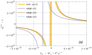
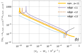
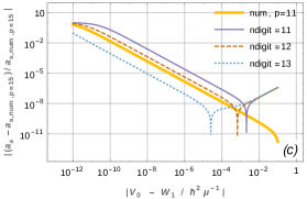
Figure 6: Importance of the location of the first pole on the accuracy of the scattering length in three dimensions. (a) $s$-wave scattering length from the numerical and the approximate expressions. In the approximate expressions, the scattering length is calculated with varying precision ($\mathrm{ndigit}$ decimal digits) of the position of the first singularity $W_{1}$. (b), (c) The errors of the approximate and numerical values of the scattering length. (b) $V_{0}<W_{1}$, (c) $V_{0}>W_{1}$ . Reference values for determining the zero points of the $x$ and $y$ axes, respectively, are calculated by numerical calculations with a high level of accuracy ($p=15$ for $a_{s}$; reference value $W_{1}=2.684004650924\hbar^{2}/\mu$).

In three dimensions the accuracy of the $s$-wave scattering length is limited mainly by the accuracy of the position $W_{1}$ of the first singularity. We determine this position using the numerical differential equation solver by finding the value of $V_{0}$ where the scattering length changes sign. The accuracy of this position can be checked by increasing the accuracy of the calculation itself. We found that $W_{1}$ can be determined with very good accuracy of 12 digits when $p=11$.

The value of $W_{1}$ can, in principle, also be obtained by diagonalizing the Hamiltonian in a plane-wave basis and determining the value of $V_{0}$ where the ground-state energy crosses zero, extrapolating to the limits of infinite box size and basis set. We found a value that is consistent with the result from the differential equation solver to three digits of accuracy, but were not able to reach higher accuracy with the diagonalization procedure due to limitations of the extrapolation procedures. Thus we have used values extracted from the differential equation solver for the numerical results presented in this paper.

The $s$-wave scattering length is plotted with different accuracy of $W_{1}$ in Fig. 6. The parameters $\alpha_{i}$ and the $W_{j}$ ($j>1$) are set according to Table 1 and are kept unchanged. The poles with the minimums on the error curves correspond to the crossing of the reference curve. The poles with the maximums come from the inaccurate position of the singularity. Increasing the accuracy of $W_{1}$ significantly improves $a_{s}^{3D}$ as well. In the main part of the paper $\mathrm{ndigit}=12$ decimal digits of accuracy are used for $W_{1}$, where the relative error is below $10^{-5}$, if the potential strength is within $W_{1}-10^{-6}\hbar^{2}/\mu<V_{0}<W_{1}+10^{-6}\hbar^{2}/\mu$.

Appendix C Alternative derivation of the approximate expressions for the $s$-wave scattering length

C.1 Three-dimensional case

Let us introduce dimensionless variables

$$y =r/L,$$ (46)

$$\eta =V_{0}\mu/\hbar^{2},$$ (47)

with which the Schrödinger equation (4) can be written in the following form:

$$\left(\frac{\mbox{d}^{2}}{\mbox{d}y^{2}}+2{y}\frac{\mbox{d}}{\mbox{d}y}+\eta\exp(-y^{2})\right)\tilde{\Phi}_{3D}(y)=E\tilde{\Phi}_{3D}(y)\ .$$ (48)

One can see from the definitions of the scattering length (6) and Eqs. (46) and (48) that the ratio $a_{s}/L$ depends only on the single dimensionless parameter $\eta$. In the following, let us consider the $E=0$ case in order to determine the $s$-wave scattering length.

The Schrödinger equation (48) can be transformed [with $\tilde{u}_{3D}(y)=y\tilde{\Phi}_{3D}(y)$] to the Lippmann-Schwinger equation Lippmann and Schwinger (1950),

$$\tilde{u}_{3D}(y)=y-\eta\int\limits_{0}^{y}\mbox{d}x\,(y-x)\exp(-x^{2})\tilde{u}_{3D}(x)\ .$$ (49)

The $s$-wave scattering length can be expressed with a simple form if we substitute Eqs. (46) and (49) into Eq. (6),

$${a}_{s}^{3D}/{L}={c_{2}}/{(c_{1}+1)}\ ,$$ (50)

where

$$c_{1} =-\eta\int\limits_{0}^{\infty}\mbox{d}x\,\exp(-x^{2})\tilde{u}_{3D}(x)\ ,$$ (51)

$$c_{2} =-\eta\int\limits_{0}^{\infty}\mbox{d}x\,x\exp(-x^{2})\tilde{u}_{3D}(x)\ .$$ (52)

Let us solve Eq. (49) with iterations. In the first step, we consider $\eta=0$ on the right hand side,

$$\tilde{u}^{(0)}_{3D}(y)=y\ .$$

Substituting it into Eqs. (50)-(52) the zero-order approximation for the scattering length can be obtained,

$$\frac{\bar{a}_{s}^{3D}}{L}=-\frac{\sqrt{\pi}}{4}\frac{\eta}{1-\frac{\eta}{2}}\ ,$$ (53)

which is equivalent to the analytical expression (24) in the main text.

C.2 One-dimensional case

In one dimension, the Lippmann-Schwinger equation and the approximate expression of the scattering length are derived analogously to the three-dimensional case,

$$\tilde{u}_{1D}(y) =1-\eta\int\limits_{0}^{y}\mbox{d}x\,(y-x)\exp(-x^{2})\tilde{u}_{1D}(x)\ ,$$ (54)

$${a}_{s}^{1D}/{L} ={(c_{2}-1)}/{c_{1}}\ ,$$ (55)

with the same relations (51) and (52) for the constants $c_{1}$ and $c_{2}$ as in the three-dimensional case. The difference from the three-dimensional solution arises from the different boundary conditions (14) and (15).

We solve Eq. (54) iteratively. In the first step we consider $\tilde{u}^{(0)}_{1D}(y)=1$, from which the first-order wave function and zero-order scattering length can be obtained,

$$\bar{u}_{1D}(y) =1-\frac{\eta}{2}\left[e^{-y^{2}}+\sqrt{\pi}y\mathop{\mathrm{erf}}(y)-1\right],$$ (56)

$$\frac{\bar{a}_{s}^{1D}}{L} =\frac{2}{\sqrt{\pi}}\frac{1}{\eta}+\frac{1}{\sqrt{\pi}}.$$ (57)

The first-order scattering length, obtained with Eq. (56), is given by

$$\frac{\bar{\bar{a}}_{s}^{1D}}{L} = \frac{2}{\sqrt{\pi}}\frac{1}{\eta}+\sqrt{\frac{2}{\pi}}+O(\eta)\ .$$ (58)

The zeroth- and first-order term recover Eqs. (28) and (29) from the main text.

C.3 Two-dimensional case

In two dimensions, the Lippmann-Schwinger equation for the function $\tilde{\Phi}_{2D}(y)$, obeying the Schrödinger equation (48), takes the form Khuri et al. (2009)

$$\tilde{\Phi}_{2D}(y)=1-\eta\int\limits_{0}^{y}\mbox{d}x\,x\ln(y/x)\exp(-x^{2})\tilde{\Phi}_{2D}(x)\ .$$ (59)

Comparing its long-range asymptotics with the definition (6) and using Eq. (46), we derive

$${{a}_{s}^{2D}}/{L}=e^{\frac{c_{1}-1}{c_{2}}-\gamma+\ln 2},$$ (60)

where

$$c_{1} =-\eta\int_{0}^{+\infty}\mbox{d}x\,\ln(x)\exp(-x^{2})\tilde{\Phi}_{2D}(x)\ ,$$ (61)

$$c_{2} =-\eta\int_{0}^{+\infty}\mbox{d}x\,x\exp(-x^{2})\tilde{\Phi}_{2D}(x)\ .$$ (62)

Similar to the previous sections, the zero-order approximation for the scattering length is obtained with the zero-order function $\tilde{\Phi}^{(0)}_{2D}(x)=1$,

$$\bar{a}_{s}^{2D}/{L} = 2e^{\frac{-3\gamma}{2}+\frac{2}{\eta}}\ .$$ (63)

The first-order wave function, obtained with the first iteration, is given by

$$\bar{\tilde{\Phi}}_{2D}(y) = 1-\frac{\eta}{4}\left[\gamma+2\ln(y)-\mbox{Ei}\left(-y^{2}\right)\right]\ ,$$ (64)

where Ei$(z)=-\int_{-z}^{\infty}\frac{e^{-t}}{t}\mbox{d}t$ is the exponential integral function. Substituting it into Eqs. (61) and (62), and using (60), gives us

$${\bar{\bar{a}}_{s}^{2D}}/{L} = \sqrt{8}e^{\frac{-3\gamma}{2}+\frac{2}{\eta}+O(\eta)}\ .$$ (65)

As can be seen the obtained Eqs. (63) and (65) are equivalent to Eqs. (34) and (35) from the main text.

Appendix D Derivation of approximate formula (29) for the one-dimensional $s$-wave scattering length

As we previously discussed in Appendix A, the one-dimensional wave function $u_{1D}(r)$ is even, hence, its power-series expansion can be written in the following form:

$$u_{1D}(r)=\sum_{k=1}^{\infty}b_{k}r^{2k}\ .$$ (66)

Substituting back Eq. (66) into Eq. (12), we got the following differential equation:

$$u_{1D}^{\prime\prime}(r)=-V_{0}e^{-r^{2}}\sum_{k=1}^{\infty}b_{k}r^{2k}\ ,$$ (67)

where $b_{0}$ is chosen to be one due to the boundary condition (14). Using the usual Taylor-expansion identity as

$$b_{k}=\frac{1}{(2k)!}\left.\frac{\mbox{d}^{2k}u_{1D}(r)}{\mbox{d}r^{2k}}\right|_{r=0}\ ,$$

the parameters can be determined from Eq. (67) or its corresponding derivative form as

$$b_{k}=-\frac{V_{0}}{(2k)!}\sum_{l=0}^{k-1}{\Bigg{[}} \binom{2k-2}{2l}\cdot$$

$$\cdot\left(2k-2-2l\right)!\ b_{k-l-1}\left.\frac{\mbox{d}^{2k}}{\mbox{d}r^{2k}}e^{-r^{2}}\right|_{r=0}{\Bigg{]}}\ .$$

Using the following identities of the Hermite polynomials:

$$\left.\frac{\mbox{d}^{2k}}{\mbox{d}r^{2k}}e^{-r^{2}}\right|_{r=0}={\mathcal{H}}_{2k}(0)=(-1)^{k}\frac{(2k)!}{k!}\ ,$$

parameter $b_{k}$ can be expressed as a linear combination of $b_{m}$ ($m<k$) as

$$b_{k}=\frac{V_{0}}{2k(2k-1)}\sum_{l=0}^{k-1}(-1)^{l+1}\frac{b_{k-1-l}}{l!}\ .$$ (68)

With Eq. (68), all the $b_{k}$ can be determined, hence function $u_{1D}(r)$ can be given explicitly in the power-series form.

In order to determine the $s$-wave scattering length, function $u_{1D}(r)$ should be examined in the asymptotic limit $r\rightarrow\infty$, which is difficult to handle in Eq. (66). However, a different form of $u_{1D}(r)$ can be considered as

$$u_{1D}(r)= 1+V_{0}c_{0}-$$ (69)

$$-V_{0}\left(e^{-r^{2}}\sum_{k=0}^{\infty}c_{k}r^{2k}+d\sqrt{\pi}\,r\,\mbox{erf}\left(r\right)\right)\ ,$$

where $c_{k}$ and $d$ are real coefficients. Equation (69) satisfies the Schrödinger equation (12), if the coefficients $c_{k}$ and $d$ are chosen properly. We can make a relation between Eqs. (67) and (69) by expanding in Taylor series of Eq. (69), where we obtain the following relations:

$$b_{0} = -2c_{0}+2c_{1}+4d\ ,$$

$$b_{1} = 4c_{0}-10c_{1}+12c_{2}-4d\ ,$$ (70)

$$b_{i+1} = 4c_{i}-2(4i+5)c_{i+1}+2(i+2)(2i+3)c_{i+2}\ ,$$

where $i\geq 1$. Considering the asymptotic limit of $r\rightarrow\infty$ in Eq. (69), the scattering length can be determined as

$$u_{1D}(r)\approx-d\sqrt{\pi}V_{0}\left(r-\underbrace{\frac{1+V_{0}c_{0}}{d\sqrt{\pi}V_{0}}}_{a_{s}^{1D}}\right)\ .$$ (71)

As can be seen in Eq. (71), $a_{s}^{1D}$ depends on only two parameters: $c_{0}$ and $d$. However, these parameters are determined through an infinitely large system of linear equations (70). The $s$-wave scattering length can be further separated into two terms as

$$a_{s}^{1D}=\frac{2}{\sqrt{\pi}V_{0}}+\underbrace{\frac{1+V_{0}c_{0}-2d}{d\sqrt{\pi}V_{0}}}_{a_{sc}^{1D}}\ .$$ (72)

Considering only the first few terms of the summation in Eq. (67), the explicit values of the parameters $c_{k}$ and $d$ can be obtained assuming the following expressions:

$$c_{0} = \frac{1}{2}+\sum_{k=1}^{\infty}\frac{k!}{2}b_{k}\ ,$$ (73)

$$d = \frac{1}{2}+\sum_{k=1}^{\infty}\frac{(2k-1)!!}{2^{k+1}}b_{k}\ .$$ (74)

These statements can be proofed by induction. First, we suppose that Eqs. (73) and (74) are true up to the first $n$th terms as

$$c_{0}^{(n)} = \frac{1}{2}+\sum_{k=1}^{n}\frac{k!}{2}b_{k}\ ,$$ (75)

$$d^{(n)} = \frac{1}{2}+\sum_{k=1}^{n}\frac{(2k-1)!!}{2^{k+1}}b_{k}\ ,$$ (76)

where parameters $c_{0}^{(n)}$ and $d^{(n)}$ gives back the original parameters $c_{0}$ and $d$ as $n$ goes to infinity. Considering a finite number of $b_{k}$, Eq. (70) terminates with the following last two equations:

$$b_{n-1} = 4c_{n-2}^{(n)}-2(4n-3)c_{n-1}^{(n)}\ ,$$ (77)

$$b_{n} = 4c_{n-1}^{(n)}\ .$$ (78)

Increasing $n$ to $n+1$$b_{k}$, Eqs. (77) and (78) are supplemented with additional terms as

$$b_{n-1} = 4c_{n-2}^{(n+1)}-2(4n-3)c_{n-1}^{(n+1)}+$$

$$\hskip 71.13188pt+2(2n-1)nc_{n}^{(n+1)}\ ,$$

$$b_{n} = 4c_{n-1}^{(n+1)}-2(4n+1)c_{n}^{(n+1)}\ ,$$ (80)

$$b_{n+1} = 4c_{n}^{(n+1)}\ .$$ (81)

Let us express $c_{n}^{(n+1)}$ in Eq. (81) and substitute back to Eqs. (D) and (80). If we introduce the following notations:

$$b_{n-1}^{\prime} =b_{n-1}-\frac{(2n-1)n}{2}b_{n+1}\ ,$$ (82)

$$b_{n}^{\prime} =b_{n}+\frac{4n+1}{2}b_{n+1}\ ,$$ (83)

then Eqs. (D) and (80) can be expressed in the following form:

$$b_{n-1}^{\prime} = 4c_{n-2}^{(n+1)}-2(4n-3)c_{n-1}^{(n+1)}\ ,$$ (84)

$$b_{n}^{\prime} = 4c_{n-1}^{(n+1)}\ .$$ (85)

Therefore, by recognizing the similarity between the expressions (84) and (85), and (77) and (78), the equations (73) and (74) for $c_{0}^{(n+1)}$ and $d^{(n+1)}$ can be extended for the $n+1$ case as

$$c_{0}^{(n+1)} = \frac{1}{2}+\sum_{k=1}^{n-2}\frac{k!}{2}b_{k}+$$

$$+\frac{(n-1)!}{2}b_{n-1}^{\prime}+\frac{n!}{2}b_{n}^{\prime}\ ,$$

$$d^{(n+1)} = \frac{1}{2}+\sum_{k=1}^{n-2}\frac{(2k-1)!!}{2^{k+1}}b_{k}+$$

$$+\frac{(2n-3)!!}{2^{n}}b_{n-1}^{\prime}+\frac{(2n-1)!!}{2^{n+1}}b_{n}^{\prime}\ .$$

Substituting back Eqs. (82) and (83) into Eqs. (D) and (D), we obtain back Eqs. (75) and (76), but the sum goes until $n+1$ justifying Eqs. (73) and (74).

Therefore, using Eqs. (73) and (74), the correction for the scattering length (72) can be explicitly given in the following form:

$$a_{sc}^{1D} = \frac{1+\sum\limits_{k=1}^{\infty}\left(k!b_{k}-\frac{(2k-1)!!}{2^{k-1}}\frac{b_{k}}{V_{0}}\right)}{\sqrt{\pi}\left(1+\sum\limits_{l=1}^{\infty}\frac{(2l-1)!!}{2^{l}}b_{l}\right)}\ .$$

Considering the limit $V_{0}\rightarrow 0$, the following identities can be derived from Eq. (68):

$$\lim_{V_{0}\rightarrow 0}b_{k} = 0\ ,$$

$$\lim_{V_{0}\rightarrow 0}\frac{b_{k}}{V_{0}} = \frac{(-1)^{k}}{2(2k-1)k!}\ .$$

Using the expression above the $a_{sc}^{1D}$ can be expressed in the following simple form:

$$\lim_{V_{0}\rightarrow 0}a_{sc}^{1D} = \frac{1}{\sqrt{\pi}}\left(1+\sum_{k=1}^{\infty}(-1)^{k+1}\frac{(2k-3)!!}{(2k)!!}\right)=\sqrt{\frac{2}{\pi}}\ ,$$

where in the last equation we recognize the Taylor series of $\sqrt{1+x}$ at $x=1$.

References

- Pethick and Smith (2002) C.J. Pethick and H. Smith, Bose-Einstein Condensation in Dilute Gases, 1st ed. (Cambridge University Press, Cambridge, 2002).
- Pitaevskii and Stringari (2016) Lev Pitaevskii and Sandro Stringari, Bose-Einstein Condensation and Superfluidity (Clarendon, Oxford, 2016).
- Roger G. Newton (1982) Roger G. Newton, Scattering Theory of Waves and Particles, 2nd ed. (Springer Science+Business Media, New York, 1982).
- Esry and Greene (1999) B.D. Esry and C.H. Greene, “Validity of the shape-independent approximation for Bose-Einstein condensates,” Physical Review A 60, 1451 (1999).
- Rontani et al. (2017) Massimo Rontani, G Eriksson, S Åberg, and S M Reimann, “On the renormalization of contact interactions for the configuration-interaction method in two-dimensions,” Journal of Physics B: Atomic, Molecular and Optical Physics 50, 065301 (2017).
- Doganov et al. (2013) R.A. Doganov, S. Klaiman, O.E. Alon, A.I. Streltsov, and L.S. Cederbaum, “Two trapped particles interacting by a finite-range two-body potential in two spatial dimensions,” Physical Review A 87, 033631 (2013).
- von Stecher et al. (2008) J. von Stecher, C.H. Greene, and D. Blume, “Energetics and structural properties of trapped two-component Fermi gases,” Physical Review A 77, 043619 (2008).
- Blume (2012) D. Blume, “Few-body physics with ultracold atomic and molecular systems in traps,” Rep.Prog.Phys. 75, 046401 (2012).
- Bugnion et al. (2014) P. O. Bugnion, P. Lopez Rios, R. J. Needs, and G. J. Conduit, “High-fidelity pseudopotentials for the contact interaction,” Physical Review A 90, 033626 (2014).
- Whitehead et al. (2016) T. M. Whitehead, L. M. Schonenberg, N. Kongsuwan, R. J. Needs, and G. J. Conduit, “Pseudopotential for the two-dimensional contact interaction,” Phys. Rev. A 93, 042702 (2016).
- Forbes et al. (2011) Michael McNeil Forbes, Stefano Gandolfi, and Alexandros Gezerlis, “Resonantly Interacting Fermions in a Box,” Physical Review Letters 106, 235303 (2011).
- Galea et al. (2016) Alexander Galea, Hillary Dawkins, Stefano Gandolfi, and Alexandros Gezerlis, “Diffusion Monte Carlo study of strongly interacting 2d Fermi gases,” Physical Review A 93, 023602 (2016).
- Christensson et al. (2009) J. Christensson, C. Forssen, S. Åberg, and S.M. Reimann, “Effective-interaction approach to the many-boson problem,” Physical Review A 79, 012707 (2009).
- Klaiman et al. (2014) Shachar Klaiman, Axel U. J. Lode, Alexej I. Streltsov, Lorenz S. Cederbaum, and Ofir E. Alon, “Breaking the resilience of a two-dimensional Bose-Einstein condensate to fragmentation,” Physical Review A 90, 043620 (2014).
- Beinke et al. (2015) Raphael Beinke, Shachar Klaiman, Lorenz S. Cederbaum, Alexej I. Streltsov, and Ofir E. Alon, “Many-body tunneling dynamics of Bose-Einstein condensates and vortex states in two spatial dimensions,” Physical Review A 92, 043627 (2015).
- Imran and Ahsan (2015) Mohd. Imran and M. A. H. Ahsan, “Exact Diagonalization Study of Bose-Condensed Gas with Finite-Range Gaussian Interaction,” Advanced Science Letters 21, 2764–2767 (2015).
- Bolsinger et al. (2017a) V. J. Bolsinger, S. Krönke, and P. Schmelcher, “Beyond mean-field dynamics of ultra-cold bosonic atoms in higher dimensions: facing the challenges with a multi-configurational approach,” Journal of Physics B: Atomic, Molecular and Optical Physics 50, 034003 (2017a).
- Bolsinger et al. (2017b) V. J. Bolsinger, S. Krönke, and P. Schmelcher, “Ultracold bosonic scattering dynamics off a repulsive barrier: Coherence loss at the dimensional crossover,” Phys. Rev. A 96, 013618 (2017b).
- (19) Aaron Farrell and Brandon P. van Zyl, “s-wave scattering and the zero-range limit of the finite square well in arbitrary dimensions,” arXiv: , 1009.1918.
- Landau and Lifshitz (1977) L. D. Landau and E. M. Lifshitz, Course of Theoretical Physics - Quantum Mechanics, Non-relativistic theory, 3rd ed., Vol. 3 (Pergamon, Oxford, 1977).
- Verhaar et al. (1985) B. J. Verhaar, L. P. H. de Goey, J. P. H. W. van den Eijnde, and E. J. D. Vredenbregt, “Scattering length and effective range for scattering in a plane and in higher dimensions,” Physical Review A 32, 1424–1429 (1985).
- Galea et al. (2017) Alexander Galea, Tash Zielinski, Stefano Gandolfi, and Alexandros Gezerlis, “Fermions in two dimensions: Scattering and many-body properties,” Journal of Low Temperature Physics 189, 451–469 (2017).
- Parish et al. (2005) Meera M. Parish, Bogdan Mihaila, Eddy M. Timmermans, Krastan B. Blagoev, and Peter B. Littlewood, “BCS-BEC crossover with a finite-range interaction,” Physical Review B 71, 064513 (2005).
- Johnson et al. (2012) P. R. Johnson, D. Blume, X.Y. Yin, W. F. Flynn, and E. Tiesinga, “Effective renormalized multi-body interactions of harmonically confined ultracold neutral bosons,” New Journal of Physics 14, 053037 (2012).
- Busch et al. (1998) T. Busch, B.G. Englert, K. Rzazewski, and M. Wilkens, “Two Cold Atoms in a Harmonic Trap,” Foundations of Physics 28, 4 (1998).
- Farrell and van Zyl (2010) Aaron Farrell and Brandon P. van Zyl, “Universality of the energy spectrum for two interacting harmonically trapped ultra-cold atoms in one and two dimensions,” Journal of Physics A 43, 015302 (2010).
- Case (1950) K. M. Case, “Singular potentials,” Phys. Rev. 80, 797–806 (1950).
- Frank et al. (1971) William M. Frank, David J. Land, and Richard M. Spector, “Singular potentials,” Rev. Mod. Phys. 43, 36–98 (1971).
- Andrews (1976) M. Andrews, “Singular potentials in one dimension,” Am. J. Phys. 44, 1064–1066 (1976).
- (30) The radial Schrödinger equation (4), and the asymptotic -wave scattering length expressions (6)-(9), are written in different forms in Ref. [20]. Using the relation , these expressions can be easily derived from each other.
- (31) The definition of differs from the original definition of Verhaar al. Verhaar et al. (1984) with an factor. The current definition is more favorable in the recent ultracold-atomic literature Levinsen and Parish (2015); Fenech et al. (2016); Boettcher et al. (2016).
- Wolfram Research, Inc. (2014) Wolfram Research, Inc., “Computer code mathematica 10.0,” (2014).
- Flügge (1999) Siegfried Flügge, Practical Quantum Mechanics (Springer, Berlin, 1999).
- Perelomov and Zel’dovich (1998) Askold M. Perelomov and Yakov B. Zel’dovich, Quantum Mechanics – Selected Topics (World Scientific, Singapore, 1998).
- Cherny and Shanenko (2001) Alexander Yu. Cherny and A. A. Shanenko, “Dilute Bose gas in two dimensions: Density expansions and the Gross-Pitaevskii equation,” Physical Review E 64, 027105 (2001).
- Lippmann and Schwinger (1950) B. A. Lippmann and Julian Schwinger, “Variational principles for scattering processes. i,” Phys. Rev. 79, 469–480 (1950).
- Khuri et al. (2009) N. N. Khuri, André Martin, J.-M. Richard, and Tai Tsun Wu, “Low-energy potential scattering in two and three dimensions,” J. Math. Phys. 50, 072105 (2009).
- Verhaar et al. (1984) B. J. Verhaar, J. P. H. W. van den Eijnde, M. A. J. Voermans, and M. M. J. Schaffrath, “Scattering length and effective range in two dimensions: application to adsorbed hydrogen atoms,” Journal of Physics A 17, 595–598 (1984).
- Levinsen and Parish (2015) Jesper Levinsen and Meera M. Parish, “Strongly interacting two-dimensional Fermi gases,” in Annual Review of Cold Atoms and Molecules, Vol. 3, edited by Kirk W. Kirk W Madison, Kai Bongs, Lincoln D Carr, Ana Maria Rey, and Hui Zhai (World Scientific, 2015) pp. 1–75.
- Fenech et al. (2016) K. Fenech, P. Dyke, T. Peppler, M.G. Lingham, S. Hoinka, H. Hu, and C. J. Vale, “Thermodynamics of an attractive 2d Fermi gas,” Physical Review Letters 116, 045302 (2016).
- Boettcher et al. (2016) I. Boettcher, L. Bayha, D. Kedar, P. A. Murthy, M. Neidig, M. G. Ries, A. N. Wenz, G. Zurn, S. Jochim, and T. Enss, “Equation of state of ultracold fermions in the 2d BEC-BCS crossover region,” Physical Review Letters 116, 045303 (2016).