Resonance dynamics of DCO ($\widetilde{X}\,{}^{2}A^{\prime}$) simulated with the dynamically pruned discrete variable representation (DP-DVR)

Abstract

Selected resonance states of the deuterated formyl radical in the electronic ground state $\widetilde{X}\,{}^{2}A^{\prime}$ are computed using our recently introduced dynamically pruned discrete variable representation (DP-DVR) [H. R. Larsson, B. Hartke and D. J. Tannor, J. Chem. Phys., 145, 204108 (2016)]. Their decay and asymptotic distributions are analyzed and, for selected resonances, compared to experimental results obtained by a combination of stimulated emission pumping (SEP) and velocity-map imaging of the product D atoms. The theoretical results show good agreement with the experimental kinetic energy distributions. The intramolecular vibrational energy redistribution (IVR) is analyzed and compared with previous results from an effective polyad Hamiltonian. Specifically, we analyzed the part of the wavefunction that remains in the interaction region during the decay. The results from the polyad Hamiltonian could mainly be confirmed. The C=O stretch quantum number is typically conserved, while the D-C=O bend quantum number decreases. Differences are due to strong anharmonic coupling such that all resonances have major contributions from several zero-order states. For some of the resonances, the coupling is so strong that no further zero-order states appear during the dynamics in the interaction region, even after propagating for 300 ps.

I Introduction

One of the fundamental processes in molecular reaction dynamics is the unimolecular dissociation of vibrationally excited molecules.Robinson and Holbrook (1972); Baer and Hase (1996); Schinke (1995); Stumpf et al. (1995) Depending on the molecular system, their decay dynamics can span the range from mode-specific to statistical. For intermediate cases, the dissociation mechanism in terms of intramolecular vibrational energy redistribution (IVR) of bound and metastable resonance states provides considerable insight into the dynamic properties of the molecular system under study. In the following, we use the term “resonance” both for vibrational resonances and metastable states. The meaning should be clear from the context and typically it will mean metastable state. Otherwise, we will point out the meaning.

One standard benchmark system is the formyl radical HCO which plays an important role in many combustion processes as well as in atmospheric and interstellar chemistry; see, e.g., LABEL:\cite[citenum]{\@@bibref{Number}{missing}{}{}}hco_astro_ocana_2017. In its electronic ground state $\widetilde{X}\,{}^{2}A^{\prime}$, HCO shows many resonance states whose decays follow very systematic mode-specific pathways.

In contrast to HCO, its deuterated counterpart DCO shows more statistical behavior. This is due to an accidental, strong $\nu_{1}\!:\!\nu_{2}\!:\!\nu_{3}\!\approx\!1\!:\!1\!:\!2$ Fermi (vibrational) resonance in the D-CO stretching vibration $\nu_{1}$ ($1910\,\mathrm{cm^{-1}}$), the DC=O stretching vibration $\nu_{2}$ ($1795\,\mathrm{cm^{-1}}$), and the D-C=O bending vibration $\nu_{3}$ ($847\,\mathrm{cm^{-1}}$). The Fermi resonance leads to strong mixing between zero-order states, already for the lowest vibrational states.Stöck et al. (1997); Keller et al. (1997); Troellsch and Temps (2001); Jung, Taylor, and Atilgan (2002) Strong mixing is an essential prerequisite for statistical dynamics. Keller et al. thus consider DCO a “precursor of ‘chaos’ in more complicated systems”.Keller et al. (1997) Consequentially, the normal assignments in terms of the associated vibrational quantum numbers ($v_{1}$, $v_{2}$, $v_{3}$) loose their meanings, although they may still be used economically as “nominal labels” to indicate possible predominating vibrational character. The only conserved quantity at short times is the polyad quantum number, $P=v_{1}+v_{2}+v_{3}/2$, which describes the total vibrational excitation.Dübal and Quack (1984); Amrein, Dübal, and Quack (1985); Kellman and Tyng (2007); Stöck et al. (1997)

Due to their strikingly different characteristics, there has been strong interest in both HCO and DCO, from both experiment and theory. Due to the amount of work on these systems, we briefly mention only some of the most important contributions. Energies and widths of resonances of HCO and DCO have been measured to high resolution by dispersed fluorescence and stimulated emission pumping.Adamson, Zhao, and Field (1993); Neyer et al. (1993); Tobiason, Dunlop, and Rohlfing (1995a, b); Stöck et al. (1997); Wei et al. (2004) For HCO, Neyer et al. also measured the rovibrational product distribution of CO.Neyer et al. (1995)

Likewise, energies and widths of HCO have been computed using various methods, establishing this system as a benchmark for computing resonance states.Bowman, Bittman, and Harding (1986); Romanowski et al. (1986); Werner et al. (1995); Keller et al. (1996); Keller and Schinke (1999); Poirier and Carrington (2002); Mandelshtam and Neumaier (2002); Tremblay and Carrington (2005); Ndengué et al. (2015); Ndengué, Dawes, and Guo (2016) Rovibrational CO state distributions and resonance decays have been analyzed by various researchers, also for nonzero total angular momentum.Qi and Bowman (1996); Yang and Gray (1997); Werner et al. (1995); Keller et al. (1996); Keller and Schinke (1997); Brandt-Pollmann, Weiß, and Schinke (2001); Dixon (1992); Gray (1992) However, less attention has been paid to DCO.Wang and Bowman (1995); Stöck et al. (1997); Keller et al. (1997); Loettgers and Schinke (1997); Stamatiadis et al. (2001) Although DCO shows close to statistical behavior, it is not fully irregular. The decay constants show strong state-to-state fluctuations. Microcanonical statistical rate theory thus cannot predict the state-specific decay constants. Due to strong anharmonic couplings, an IVR analysis is much less straightforward but still desirable. Clear indications that remaining regularities may be strong enough for such an approach were provided by the aforementioned polyad model that turned out to be applicable to DCO and quite useful.Keller et al. (1997) The group of Temps fitted an effective polyad Hamiltonian to experimental data and did an analysis of different IVR pathways within this polyad model.Troellsch and Temps (2001); Renth, Temps, and Tröllsch (2003) This model Hamiltonian was then used for further semiclassical analysis.Jung, Taylor, and At$\mathrm{i}$lgan (2002); Huang and Wu (2007); Semparithi and Keshavamurthy (2003) However, many of these analyses still lack comparison with quantum calculations on an ab-initio potential energy surface (PES).

Here, we make an initial attempt to fill this gap by a joint experimental and theoretical study of the observed and calculated resonances of DCO in polyads $5$ and $5.5$. In particular, we present experimental kinetic energy release (KER) spectra of the D atoms from the decay of the resonances and the associated CO vibration-rotation product state distributions. The results were obtained using the method of Stimulated Emission Pumping (SEP)Stöck et al. (1997) for the preparation of selected excited DCO resonance states in combination with velocity-map imaging Eppink and Parker (1997) of the D atoms. In addition, we computed the CO state distributions using our dynamically pruned discrete variable representation (DP-DVR) approachHartke (2006); Larsson, Hartke, and Tannor (2016); Tannor et al. (2018) and analyzed the computed resonance decays. As critical tests of the theory, we compare our computational results with the experimental data taking either the PES of Werner et al. (WKS)Werner et al. (1995); Keller et al. (1996) or the PES of Song et al. (SAG).Song, van der Avoird, and Groenenboom (2013)

We thereby use this study as a real-life application of our new method for performing molecular quantum dynamics. The standard method in molecular quantum dynamics is to employ a direct-product basis of discrete variable representation (DVR) functions.Tannor (2007) However, this approach suffers from an exponential scaling of basis size with dimensionality. Even for lower-dimensional problems like the one studied here, it is not the most efficient method. For dissociation problems like DCO, long coordinate ranges need to be described, but the wavefunction typically does not occupy the whole direct-product coordinate space. Such a problem is well-suited for only using DVR grid points where the wavepacket has non-negligible amplitudes. This leads to significant savings in computational resources (both regarding number of operations and memory requirements). Since the wavepacket moves in time, the set of active basis functions needs to be dynamically adapted. Exactly this capability is provided by our dynamically pruned DVR approach (DP-DVR).Hartke (2006); Larsson, Hartke, and Tannor (2016); Tannor et al. (2018) The accuracy is controlled by a so-called wave-amplitude threshold.Hartke (2006); Machnes, Assémat, and Tannor (2016) The smaller the threshold, the more basis functions are added and the more accurate the simulation becomes. In LABEL:\cite[citenum]{\@@bibref{Number}{missing}{}{}}pvb_rev_tannor_2017 we have introduced a very efficient algorithm for DP simulations and have done careful benchmarks of the DP-DVR and other methods. We have shown that DP-DVR can be more efficient than conventional dynamics already for two-dimensional systems.

For the dissociation dynamics of DCO, phase-space bases would be other useful candidates for our DP approach.Shimshovitz and Tannor (2012); Machnes et al. (2016); Larsson, Hartke, and Tannor (2016); Tannor et al. (2018) One could use such a phase-space basis in the coordinate describing the dissociation. However, efficient use of phase-space bases requires that the potential operator has the form of a sum of products of one-dimensional terms (SOP form). This requires an additional fitting of the potential into this form.

Recently, we have combined our DP approach with the Multiconfiguration Time-Dependent Hartree method (MCTDH), giving DP-MCTDH.Larsson and Tannor (2017) There, DP can be used either for pruning the time-dependent basis functions (single-particle functions) or their DVR representation. The former is most useful for higher-dimensional systems (see also Refs. 52; 53; 54) whereas the latter is useful whenever many DVR functions are needed for describing the (multidimensional) single-particle functions. This is the case for DCO dissociation dynamics such that DP-MCTDH could be a useful method for our study. MCTDH itself has been used for computing resonances of HCO.Ndengué et al. (2015); Ndengué, Dawes, and Guo (2016) However, the MCTDH algorithm is more complicated than a DVR code. Furthermore, as with phase-space bases, an efficient use of MCTDH requires a SOP form of the potential. Although methods for combining arbitrary potentials with MCTDH exist,Manthe (1996); Wodraszka and Carrington (2018) they are less well established and require more careful convergence tests. Further, MCTDH is most useful for weakly correlated systems and short-time dynamics, but for HCO Ndengué et al. (2015) many single-particle functions are needed and the wavepacket has to be propagated for tens of picoseconds.

Here, we resort to our standard DP-DVR algorithm to make our simulations as simple as possible, without jeopardizing computational efficiency, and also to test the capabilities of our DP-DVR approach in an application involving resonances and their decay.

The remainder of this Article is organized as follows: The experimental and theoretical setups are described in Sections II and III, respectively. The latter provides more details on the DP-DVR method (subsection III.1), on the methods to obtain resonance states (subsection III.2) and asymptotic product distributions (subsection III.3), and on the employed PES (subsection III.4). Our results are presented and discussed in Section IV. The experimental velocity map images are presented in subsection IV.1. subsection IV.2 details the simulation parameters and subsection IV.3 compares our computed resonance energies and widths with literature values. The PES is analyzed in terms of an adiabatic picture in subsection IV.4, the experimental and theoretical asymptotic distributions are presented and compared in subsection IV.5, and the decay processes of the studied resonances are analyzed in subsection IV.6. We summarize in Section V.

II Experiment

The measurements required four spatially and temporally controlled laser pulses to be focused into a supersonic seeded molecular beam in a differentially pumped stainless steel vacuum chamber. Fig.  1 shows a sketch of the employed installation. The SEP part of the setup for preparation of the DCO ($\widetilde{X}$) radicals in their highly excited states Stöck et al. (1997); Wei et al. (2004) and the photofragment imaging part for measuring the kinetic energy release to the D atomsWei et al. (2003); Riedel et al. (2005) have been described in some detail separately before. The exact experimental conditions varied slightly from those to record optimal SEP spectra by the need of the present experiment for a high number density of highly vibrationally excited radicals.Riedel (2006)

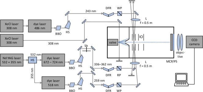
Figure 1: Schematic diagram of the experimental setup. BBO: doubling crystal, DFR: double-Fresnel rhomb, HS: harmonic separator, IO: ion optics electrode assembly, L: lens, MCP: multi-channel plate, PS: phosphor screen, RP: Rochon prism, Sh: shutter, WP: Wollaston prism.

A pulsed supersonic free jet containing $\sim 0.5\,\mathrm{\%}$ deuterated acetaldehyde (CD3CDO) in He was generated by flowing the carrier gas at a backing pressure of $\sim 2\,\mathrm{bar}$ through a stainless steel reservoir with freshly distilled CD3CDO (Fluka, $>99\,\mathrm{\%}$) at $-78\,\mathrm{{}^{\circ}{}C}$ and expanding it into the first vacuum chamber of the imaging apparatus through a 0.8 mm diameter solenoid-actuated valve (General Valve) at 20 Hz repetition rate. Photolysis of the CD3CDO with a XeCl excimer laser at $\lambda=308\,\mathrm{nm}$ in the high-pressure region of the free jet expansion $\sim 3\,\mathrm{mm}$ behind the pulsed nozzle produced the desired DCO radicals. A molecular beam of the radicals shaped by a 1.5 mm diameter conical skimmer then entered the test volume between the repeller and extractor plates of the imaging electrode assembly in the second vacuum chamber, where it was crossed by the pump, dump and probe laser beams. A liquid-N2 cryo-pump surrounding the assembly minimized the background ion signal.

Two dye lasers (Lambda Physik) were optically pumped by the dichroically separated third resp. second harmonic output beams of a Nd:YAG laser (Spectra Physics) and frequency-doubled in BBO crystals to obtain the required $\sim 259\,\mathrm{nm}$ pump (1.5 mJ) and 336 – 362 nm dump (5 – 7 mJ) pulses. The precise wavelengths were set by recording the $\widetilde{B}(^{2}A^{\prime})\leftarrow\widetilde{X}(^{2}A^{\prime})$ fluorescence excitation and $\widetilde{B}\rightarrow\widetilde{X}$ SEP spectra in a separate molecular beam apparatus with fluorescence detection. Stöck et al. (1997); Wei et al. (2004) Both beams were focused into the test volume at a small angle with respect to each other through a $f=500\,\mathrm{mm}$ fused silica lens. The 308 nm excimer-pumped probe dye laser (both Lambda Physik) for imaging of the D atoms from the D-CO dissociation reaction by 2+1 resonance-enhanced multi-photon ionization (REMPI) via the $2\,{}^{2}S\leftarrow 1\,{}^{2}S$ transition was frequency-doubled to the required $\lambda=243\,\mathrm{nm}\ (1\,\mathrm{mJ})$ and focused into the detection region counter-propagating to the pump and dump with a short delay of $\sim 10\,\mathrm{ns}$. The exact probe wavelength was set by optimizing the D^+ ion yield. All laser polarizations were set parallel to the plane of the imaging detector using combinations of Fresnel double rhombs and Rochon or Wollaston prisms.

The imaging measurements were made under velocity mapping conditions. Eppink and Parker (1997) The probe laser was periodically scanned over the Doppler profile of the recoiling D atoms. The resulting D^+ ions were monitored on a microchannel plate (MCP) detector coupled to a phosphor screen. The obtained signals were recorded on a CCD camera and accumulated over up to $200\,000$ laser shots using single ion counting and centroiding Chang et al. (1998) to improve the detection sensitivity and spatial resolution and to discriminate against noise. Background images with the dump laser blocked on alternate shots were subtracted to eliminate contributions to the D atoms from the CD3CDO photolysis and from predissociation of the DCO ($\widetilde{B}$) state. Mass selectivity was achieved using a fast transistor switch (Behlke) to gate the MCP. The timing of the pulsed valve, all lasers and the MCP voltage was controlled by a digital delay generator (Stanford Research).

III Theory

III.1 Dynamically pruned discrete variable representation (DP-DVR)

The propagation is performed in Jacobi coordinates $\{R,r,\theta\}$. $R$ is the distance of D to the center of mass of C-O, $r$ is the C-O distance and $\theta$ the angle between the corresponding vectors $\vec{R}$ and $\vec{r}$. As usual,Le Quéré and Leforestier (1990) the wavefunction is divided by $Rr$ such that the volume element takes the form of $\mathrm{d}V=\mathrm{d}R\,\mathrm{d}r\,\sin(\theta)\mathrm{d}\theta$. In our propagation, we consider only the $\widetilde{X}\,{}^{2}A^{\prime}$ ground state and neglect nonadiabatic and Renner-Teller couplings. The couplings only play an important role if the wavefunction has non-negligible contributions at linear geometries.Werner et al. (1995) This requires high excitation in the bending mode and only occurs for a minority of the resonances studied; we will mention them in subsection IV.6.

The wavefunction is represented by a Gauß-Legendre DVR for the angular coordinate and by a sinc DVR for the radial coordinates.Tannor (2007); Colbert and Miller (1992) This direct-product basis is then pruned using our DP-DVR approach,Larsson, Hartke, and Tannor (2016) which is related to previous pruning methods.Hartke (2006); Sielk et al. (2009); Pettey and Wyatt (2006, 2007); McCormack (2006) In contrast to those, we could show that our approach is actually faster than conventional methods. If the absolute value of a coefficient of a direct-product basis function is larger than a predefined wave-amplitude threshold, this basis function and its nearest neighbors become active. Otherwise, this function is removed from the set of active functions. This procedure is repeated at each time step, ensuring a compact representation of the wavefunction for all propagation times. For further details we refer to LABEL:\cite[citenum]{\@@bibref{Number}{missing}{}{}}pW_tannor_2016.

In the following, we mention two improvements of our code introduced in LABEL:\cite[citenum]{\@@bibref{Number}{missing}{}{}}pW_tannor_2016 (the reader who is not interested in technical details may skip the rest of this Subsection). The first improvement is a (straightforward) implementation of standard shared-memory parallelization. For the second improvement, we take advantage of the fact that the momentum and kinetic energy operators in sinc DVR representation give Toeplitz matrices with elements $T_{i,j}=T_{i+1,j+1}=t_{i-j}$. Instead of storing all matrix elements $T_{i,j}$, we only store one row $t_{i-j}$ of the matrix. This reduces the memory needed to be loaded into the cache of the central processing units and thus gives large speed-ups, especially for shared-memory parallelization. In standard molecular quantum dynamics applications with basis sizes smaller than 100, the storage of the one-dimensional matrices is negligible, compared to the storage of the (pruned) multidimensional wavefunction. However, the exploitation of the Toeplitz structure becomes useful whenever the one-dimensional basis size is large. This is the case for the dissociation dynamics considered here. For a basis that is not pruned, the action of a Toeplitz matrix onto a vector can be implemented with a scaling of $\mathcal{O}\bigl{(}N\log(N)\bigr{)}$ using fast Fourier transforms (FFTs).Gohberg and Olshevsky (1994) However, when the basis is pruned, some structure of the pruned matrix is lost and an implementation in terms of FFTs is not straightforward. Nevertheless, the matrix–vector product in a pruned basis is much faster than a FFT in an unpruned basis if pruning reduces the size of the objects sufficiently, which typically is the case.

III.2 Retrieval of resonances

Previously, HCO and DCO resonances have been computed using, among others, Lanczos procedures,Poirier and Carrington (2002); Tremblay and Carrington (2005) a log-derivative version of Kohn’s variational principle,Keller et al. (1997, 1996) MCTDH,Ndengué et al. (2015) projection theory,Wang and Bowman (2017) and filter diagonalization.Mandelshtam and Neumaier (2002); Brandt-Pollmann, Weiß, and Schinke (2001) Many applications utilize the time-independent Schrödinger equation (TISE). In principle, our DP-DVR code would work as well for the TISE using an algorithm that iteratively adds and removes new basis functions after each Lanczos iteration.Machnes, Assémat, and Tannor (2016) However, Lanczos and other iterative diagonalization algorithms require a good preconditioner for efficient usage,Huang and Carrington (2000); Poirier and Carrington (2001, 2002) especially when eigenstates are searched in the middle of a dense eigenspectrum, as is the case in this application. The search for a good preconditioner for a Hamiltonian is not trivial and depends on the employed basis. We tested the preconditioner proposed in LABEL:\cite[citenum]{\@@bibref{Number}{missing}{}{}}precond_huang_2000 and some standard preconditioners like diagonal matrices but found no satisfying results.

Thus, instead of using a Lanczos approach, we use filter diagonalization.Neuhauser (1990, 1991) Since the standard form of filter diagonalization is based on propagation, it allows for a straightforward integration into a DP code for solving the time-dependent Schrödinger equation. This worked without any adjustments or tuning of parameters, and the bottleneck of our simulations was then not the retrieval of the eigenstates but the subsequential simulation of their decay. Thus, we did not try to use further improvements of filter diagonalization.Takatsuka and Hashimoto (1995); Mandelshtam and Taylor (1997); Mandelshtam and Neumaier (2002)

In standard filter diagonalization, a real-time dynamics of an initial wavepacket with absorbing boundary conditions is performed and the wavepacket is stored at intermediate times. Afterwards, the wavepacket is filtered at (typically equidistantly spaced) energies $E_{n}$ via Fourier transform:Neuhauser (1991)

$$|{\Phi_{F}(E_{n})}\rangle=\frac{1}{2\pi\hbar}\int_{0}^{\infty}\exp(\mathrm{i}E_{n}t/\hbar)|{\Psi(t)}\rangle F(t)\mathrm{d}t,$$ ((1))

where $F(t)$ is a filter function of the form

$$F(t)=\exp[-(t-\tau)^{2}W^{2}/\hbar^{2}].$$ ((2))

$W$ is the energy bandwidth, here taken as $E_{n+1}-E_{n}$. The duration $\tau$ is set such that $W\tau\gg 1$. Afterwards, the Hamiltonian is represented in the nonorthogonal basis of filtered states $\{|{\Phi_{F}(E_{n})}\rangle\}_{n=1}^{N}$ and diagonalized. The size of the basis is typically less than $100$, such that diagonalization can be performed using standard procedures. The obtained eigenvalues $E_{n}$ are complex-valued, including both the resonance energies $\epsilon_{n}$ and resonance widths $\Gamma_{n}$ as $E_{n}=\epsilon_{n}-\mathrm{i}\frac{\Gamma_{n}}{2}$. In the following, the width $\Gamma$ will be used for wavenumber quantities.

III.3 Rovibrational product distribution

For obtaining the KER spectra of the D atom and the asymptotic rovibrational distributions of the CO fragment, we employ the analysis-line method developed by Balint-Kurti et al.Balint-Kurti, Dixon, and Marston (1990) It has previously been used for HCO by both Gray and Dixon.Gray (1992); Yang and Gray (1997); Dixon (1992) The retrieval of the asymptotic distribution is performed by Fourier-transforming cuts of $\Psi(R,r,\theta;t)$ along the “analysis line” $R=R_{\infty}$, where the cuts $\Psi(R_{\infty},r,\theta;t)$ are represented in the basis of asymptotic rovibrational states, $\{|{\psi_{vj}}\rangle\}$. $v$ and $j$ are the CO stretch and rotational quantum numbers, respectively. The working expression is

$$C_{vj}(R_{\infty},t) =\langle{R_{\infty}}|\langle\psi_{vj}|\,\Psi(t)\rangle,$$

$$A_{vj}(R_{\infty},E) =\frac{1}{2\pi}\int_{0}^{\infty}\exp(\mathrm{i}Et/\hbar)C_{vj}(R_{\infty},t)\mathrm{d}t.$$

The KER spectrum $P(E_{\ce{D}})$ is then given by

$$P(E_{\ce{D}}) =\sum_{v,j=0}^{\infty}P_{vj}(E_{\ce{D}}),$$ ((3))

$$P_{vj}(E_{R}) =\lim_{t\to\infty}\bigl{|}\langle\Psi^{(-)}_{kvj}|\,\Psi(t)\rangle\bigr{|}^{2}$$ ((4))

$$=\frac{16\pi^{3}k}{\mu_{R}}\left|A_{vj}(R_{\infty},E_{R})\right|^{2},$$ ((5))

$$E =E_{vj}+E_{R},\quad E_{D}=\frac{m_{\ce{CO}}}{m_{\ce{DCO}}}E_{R},$$ ((6))

where $k=\sqrt{2\mu_{R}E_{R}/\hbar^{2}}$ and $E_{R}$ is the kinetic energy in the internal Jacobi coordinate $R$. The corresponding kinetic energy of the D atom in the laboratory frame (without translation and rotation of the DCO system) is then given by mass-weighting $E_{R}$ (Eq.  (6)), as obtained from the standard center-of-mass transformation of a two-body system.Bernath (2005) $E_{vj}$ is the internal energy of the CO fragment. $\mu_{R}$ is the reduced mass of $\ce{D-CO}$ in Jacobi coordinates. $|{\Psi^{(-)}_{kvj}}\rangle$ is the outgoing scattering state for dissociation into D and CO.Schinke (1995) Integrating $P_{vj}(E_{R})$ over all $E_{R}$ gives the rovibrational distributions of the CO product.

Combining this method with our DP-DVR approach is straightforward because the only quantity that needs to be stored during the dynamics calculation is the wavefunction evaluated at $R_{\infty}$ which is a DVR grid point in the asymptote. When no basis function at $R_{\infty}$ is active at a specific time step, the wavefunction there is simply zero.

III.4 Potential energy surfaces

To the best of our knowledge, there are three accurate and more recent potential energy surfaces (PES) for HCO. The (modified) WKS surface of Werner, Keller and SchinkeWerner et al. (1995); Keller et al. (1996) has been applied in many studies; for example Refs. 6; 7; 24; 25; 26; 27; 68. This PES quite accurately describes both the dissociation and the interaction region, including the conical intersection at linear geometry. It is based on multireference configuration interaction (MRCI) calculations. Another recent PES is that developed by Song, van der Avoird and Groeneboom (SAG).Song, van der Avoird, and Groenenboom (2013) It is based on unrestricted coupled-cluster calculations and focuses on the asymptotic and lower-energy regions. It has been used for scattering calculations.Song et al. (2015) The third recent PES was developed by Ndengué, Dawes and Guo and is based on explicitly correlated MRCI calculations.Ndengué, Dawes, and Guo (2016) It was used for unraveling the effects of Renner-Teller coupling on the resonance levels.

Only the WKS surface has been used in studies of DCO.Stöck et al. (1997); Keller et al. (1997) To connect to those previous studies, we mainly use this well-established PES in our calculations. In order to estimate the sensitivity of the observables to changes of the potential, we also employed the SAG surface for selected resonances. Figures i and ii in the supplementary material show cuts of the two PES. Since none of those PES were constructed with decay dynamics of high-energy resonance states far out into the asymptote in mind, none of the utilized PES can be expected to give quantitative agreement between theoretical and experimental results in this present application.

IV Results and discussion

IV.1 Experimental Results

Four DCO ($\widetilde{X}$) resonances were picked at random for investigating the KER spectra and CO ($v,j$) product state distributions by the D atom velocity map imaging experiment. Two states were taken from polyad $P=5$ (at wavenumbers ${\tilde{\nu}_{v}}=8\,902$ and $8\,942\,\mathrm{cm^{-1}}$) and two from polyad $P=5.5$ (${\tilde{\nu}_{v}}=9\,896$ and $10\,065\,\mathrm{cm^{-1}}$). SEP spectra illustrating the observed vibrational states belonging to both polyads are shown in Fig.  2.

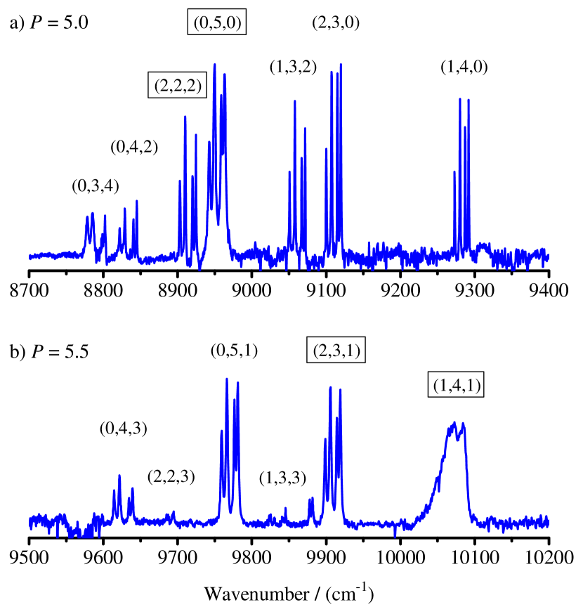
Figure 2: SEP scans over a) polyad 5.0 and b) polyad 5.5 with nominal assignments of the observed resonances according to LABEL:\cite[citenum]{\@@bibref{Number}{missing}{}{}}DCO_II_schinke. The four resonances selected for D atom imaging are highlighted by frames around the state labels. With the pump laser tuned to the $\widetilde{B}\leftarrow\widetilde{X},\ 0_{0}^{0}$, ${}^{q}R_{0}(0)$ line at $\nu_{\text{pump}}=38\,631.60\,\mathrm{cm^{-1}}$, state, the dump transition can reach four different rotational states, $N_{K_{a}K_{c}}=0_{00},\ 2_{02},\ 1_{10}$ and $2_{12}$, in each $\widetilde{X}$ vibrational state, explaining the four-line patterns observed in the SEP scans.

Following Keller et al.,Keller et al. (1997) the four resonances are nominally labeled as (0,4,2), (0,5,0), (2,3,1) and (1,4,1), in order of increasing energy for reference below. We emphasize, however, that these “assignments” have to be taken with caution. For example, the $8\,902\,\mathrm{cm^{-1}}$ resonance was reported as a mixture of 48 % (2,2,2) and 32 % (0,4,2), while the neighboring $8\,821\,\mathrm{cm^{-1}}$ resonance was found as a mixture 41 % (2,2,2) and 32 % (0,4,2). Further, the resonance at ${\tilde{\nu}_{v}}=10\,065\,\mathrm{cm^{-1}}$ nominally assigned as (1,4,1) is special because it shows pronounced interpolyad mixing with a highly dissociative resonance belonging to polyad $P=6$, most likely (4,2,0).Wei et al. (2004) We note that we use the same notation $(v_{1},v_{2},v_{3})$ for both zero-order states and resonance states. Which state is meant should either be clear from the context or the state is explicitly designated as resonance or zero-order state.

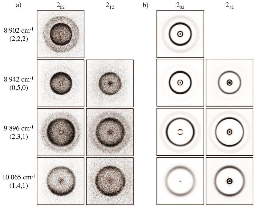
Figure 3: a) Measured two-dimensional (2D) D atom velocity map images after excitation of the (0,4,2), (0,5,0), (2,3,1) and (1,4,1) DCO ($\widetilde{X}$) resonances in the 2₀₂ and 2₁₂ rotational states and b) reconstructed meridional slices through the respective three-dimensional (3D) D atom recoil distributions.

The recorded D atom velocity mapped images after excitation of the 2₀₂ and 2₁₂ rotational states of the above four DCO ($\widetilde{X}$) resonances are printed in Fig.  3 a) together with their Abel inversions in Fig.  3 b). The depicted meridional slices through the three-dimensional (3D) D atom recoil distributions were obtained using the iterative regularization method with the projected Landweber algorithm.Renth, Riedel, and Temps (2006) As can be seen, the raw images and the associated slices through the 3D recoil distributions differ substantially from vibrational resonance to resonance, while the results for the two rotational states are very similar, indicating the good reproducibilty of the data. For (0,5,0) and (1,4,1), the 3D slices show D atoms with comparably low recoil velocities. The allowed maximal available energies $E_{\text{avl}}$ is determined by the energy balance

$$E_{r}+{\mathrm{h}(\nu_{\text{pump}}-\nu_{\text{dump}})}=\Delta{E}_{0}^{0}\text{(\ce{D-CO})}+E_{\text{avl}},$$ ((7))

where $E_{r}$ is the initial state’s rotational state (here $E_{r}=0$ for $N_{K_{a}K_{c}}=0_{00}$), $\Delta{E}_{0}^{0}\text{(\ce{D-CO})}$ is the asymptotic D-CO dissociation energy, and $\nu_{\text{pump}}$ and $\nu_{\text{dump}}$ are the frequencies supplied by the pump and dump laser pulses. Thus, dissociation of the (2,2,2) and (0,5,0) resonances may lead to CO in $v=0$ and $v=1$, while the (2,3,1) and (1,4,1) resonances may also give CO in $v=2$. Evidently, however, (0,5,0) and (1,4,1) give mainly CO in $v=1$. Further, as by the narrow recoil widths, the CO ($v=1$) acquires relatively low rotational excitation (quantum number $j$). In contrast, the images obtained from the (2,2,2) and (2,3,1) resonances show the formation of CO in $v=1$ and in $v=0$, with broader rotational excitation in $v=0$. The observed recoil anisotropies are negligible within experimental errors, consistent with resonance lifetimes ($\tau=0.8\,\text{--}\,5\,\mathrm{ps}$ inferred from the measured resonance widths) longer than the DCO rotational period.

Subsequent integration of the D atom images over the angular coordinates and transformation of the resulting recoil velocity distributions to the recoil translational energies with account of the fragment mass ratio and the appropriate Jacobian finally gave the total kinetic energy release (KER) spectra for the decaying resonances. The corresponding CO vibrational and rotational product state distributions follow by the energy balance. The experimental KER spectra will be presented and compared with the present theoretical predictions in subsection IV.5. The asymptotic D-CO dissociation energy was assumed to have a value of $\Delta{E}_{0}^{0}=5\,450\,\mathrm{{h\,c\,}cm^{-1}}$.

IV.2 Simulation parameters

For the filter diagonalization, the initial wavefunction is taken from LABEL:\cite[citenum]{\@@bibref{Number}{missing}{}{}}DCO_II_schinke and takes the form of the following Gaussian (excluding normalization)

$$\begin{split}\Psi^{\text{FD}}&(R,r,\theta;t=0)\propto\exp\{-[(R-R_{0})/\alpha_{R}]^{2}\}\\ \times&\exp\{-[(r-r_{0})/\alpha_{r}]^{2}\}\exp\{-[(\theta-\theta_{0})/\alpha_{\theta}]^{2}\},\end{split}$$ ((8))

with the parameters $R_{0}=3.05\,\mathrm{a_{0}},r_{0}=2.57\,\mathrm{a_{0}},\theta_{0}=138^{\circ},\alpha_{R}=0.256\,\mathrm{a_{0}},\alpha_{r}=0.195\,\mathrm{a_{0}},$ and $\alpha_{\theta}=7.19^{\circ}$. This initial wavepacket is propagated for $2\,\mathrm{ps}$. The filter function is a Gaussian with duration of $\tau=1\,\mathrm{ps}$ (see Eq.  (2)), and the energy region of interest (see subsection IV.3) was divided into four regions, each with a width of $\sim 400\,\mathrm{{h\,c\,}cm^{-1}}$ and with typically $10$ energy-filtered basis functions. For each region, the number of basis functions was adapted to avoid an overcomplete basis.

The DVR basis set parameters are given in Table 1. For the filter diagonalization, a smaller range in $R$ up to $R=10\,\mathrm{a_{0}}$ is used. Due to a wrong asymptote of the SAG potential, a smaller coordinate range in $r$ was used for all simulations on that PES. In coordinate $R$, we use the transmission-free complex absorbing potential (CAP) of LABEL:\cite[citenum]{\@@bibref{Number}{missing}{}{}}cap_manolopoulos_2002 (taking the rational form, Eq. (2.25) in that reference) with a width of $5\,\mathrm{a_{0}}$ for the filter diagonalization and a width of $10\,\mathrm{a_{0}}$ for the decay dynamics. This corresponds to starting positions of the CAP at $5\,\mathrm{a_{0}}$ and $18\,\mathrm{a_{0}}$, respectively. Similar values have been used previously for obtaining resonance states.Keller et al. (1997); Ndengué et al. (2015); Tremblay and Carrington (2005) For selected states, we have done simulations with other CAP positions and widths and found no significant deviations for neither the resonance energies/widths nor the decay distributions. We use the following atomic masses: $12.0096\,\mathrm{Da}$ for C,Meija et al. (2016) $15.99977\,\mathrm{Da}$ for O and $2.01410178\,\mathrm{Da}$ for D.Wang et al. (2017)

The wave-amplitude threshold used for the pruning of the filter diagonalization dynamics is $10^{-11}$, although a threshold of $10^{-8}$ would give the same results. This looser threshold is used for the decay dynamics. There, a threshold of $10^{-6}$ would have been sufficient. The analysis line (subsection III.3) is placed at $R_{\infty}=16\,\mathrm{a_{0}}$. For all propagations, we employ a short iterative Arnoldi propagatorPark and Light (1986); Beck et al. (2000) with an accuracy of $10^{-10}$, in the form in which it is also implemented in the Heidelberg MCTDH package.Worth et al. For each resonance, the final propagation time and the norm of the wavefunction at that time can be found in Table i in the supplementary material.

We note that all parameters were chosen conservatively and are not well-optimized. Especially, the employed coordinate ranges are probably too large. They do not require an in-depth optimization because our DP algorithm does this automatically: If the wavepacket will not enter a certain region in coordinate space, no basis function will become active in that region during the propagation and computational costs will not increase, compared to a carefully optimized coordinate range. Further, this means that the CAP width needs not be tuned to increase computational efficiency (although, the stronger the CAP, the earlier the wavefunction is absorbed in the CAP region, and the fewer basis functions are needed). This gives the DP-DVR algorithm more of black-box character than conventional DVR dynamics. However, the other parameters still required convergence tests. The number of DVR functions, which determines the maximum momentum that can be described, can be easily determined by checking reduced densities of the wavefunction in momentum space. For the filter diagonalization and decay dynamics of selected resonances, careful convergence tests with tighter parameters have been pursued and the stated final parameters, including $R_{\infty}$, were chosen based on conservative conclusions from these tests.

Table 1: Basis sizes $N$ and coordinate ranges for the three Jacobi coordinates $R,r$ and $\theta$ for the two employed PES. The values in the ranges are given in units of the Bohr radius $a_{0}$.Stohner and Quack (2011)

	$R$		$r$		$\theta$
PES	$N$	range	$N$	range	$N$	range
WKSWerner et al. (1995); Keller et al. (1996)	210	$[1.5,28]$	78	$[1.5,6]$	60	$[0,\pi]$
SAGSong, van der Avoird, and Groenenboom (2013)	-"-	-"-	34	$[1.5,3.49]$	-"-	-"-

IV.3 Energies and widths

The computed resonance energies and widths on the WKS surface are given in Table 2 and compared with both the experimental and theoretical values from Refs. 6; 7.

Note that some energetically low-lying resonances (below ${\tilde{\nu}}=8770\,\mathrm{cm^{-1}}$, ${\tilde{\nu}}$ is the vibrational resonance wavenumber relative to the ground state) in polyad $5$ and one in polyad $5.5$ are not included in our simulations. They were also not experimentally accessible. Here, we consider resonances in polyad $5$ and $5.5$ that are within a range of $8770\,\mathrm{cm^{-1}}$ and $10050\,\mathrm{cm^{-1}}$.

Compared to the computed wavenumbers from LABEL:\cite[citenum]{\@@bibref{Number}{missing}{}{}}DCO_II_schinke, ours are systematically smaller but agree within $\sim 5\,\mathrm{cm^{-1}}$. The decay widths have a better agreement; there, except for resonance (0,3,4), the maximal absolute deviation is $1\,\mathrm{cm^{-1}}$. Note that Keller et al. reported that their basis was probably too small to yield accurate calculations.Keller et al. (1997) Their basis used in the calculations for HCOKeller et al. (1996) was significantly larger. To our knowledge, there are no further calculations done for DCO on the WKS surface. However, theoreticians have used resonance calculations for HCO on the WKS surface as a benchmark case.Keller and Schinke (1999); Poirier and Carrington (2002); Mandelshtam and Neumaier (2002); Tremblay and Carrington (2005); Ndengué et al. (2015); Ndengué, Dawes, and Guo (2016) There, the deviations from the results of LABEL:\cite[citenum]{\@@bibref{Number}{missing}{}{}}HCO_II_schinke have a similar magnitude as the deviations shown here. To conclude, our DP-DVR method with filter diagonalization gives results that are within reasonable agreement with the results from Keller et al. To allow for a better comparison, more extensive tests with HCO should be done but this is not within the scope of this work.

Table 2: Comparison of computed resonance transition wavenumbers $\tilde{\nu}$ (relative to the ground state) and widths $\Gamma$ from this work (DP) with the experimental (Exp.) and theoretical (WKS) results from Refs. 6; 7.

		$\tilde{\nu}/\mathrm{cm^{-1}}$				$\Gamma/\mathrm{cm^{-1}}$
P.	label	Expt.	WKS	DP	$\Delta$	Expt.	WKS	DP	$\Delta$	decomposition of wavefunction
5	((034))	8778	8780	8775	5	3.50	$7.6$	$5.6$	2	38:	034	30:	(411)	16:	222	16:	124
5	((042))	8821	8832	8830	2	<2.00	$1.1$	$1.1$	0	41:	222	32:	042	23:	132
5	((222))	8902	8901	8895	6	1.06	$1.9$	$1.2$	0.7	48:	222	32:	042
5	(050)	8942	8953	8950	3	1.79	$0.14$	$0.13$	0.01	44:	050	33:	(140)	15:	230
5	(132)	9050	9031	9029	2	0.34	$0.28$	$0.28$	0	59:	132	24:	042	11:	222
5	(230)	9099	9099	9096	3	0.20	$0.32$	$0.32$	0	57:	230	32:	050
5.5	027	—	9235	9234	1	—	$14$	$13$	1	100:	027
5	((140))	9272	9251	9248	3	0.29	$0.32$	$0.31$	0.01	64:	140	20:	230	14:	050
5.5	((321))	—	9496	9494	2	—	$17$	$17$	0	57:	(321)	32:	035
5.5	(043)	9614	9630	9629	1	2.30	$1.5$	$1.4$	0.1	38:	(223)	29:	043	27:	133
5.5	(223)	9686	9690	9688	2	<5.00	$5.6$	$5.5$	0.1	52:	(223)	25:	043	13:	035
5.5	((051))	9757	9764	9762	2	0.83	$0.66$	$0.64$	0.02	26:	051	24:	231	22:	141	22:	043
5.5	((133))	9819	9807	9805	2	<3.00	$1.9$	$1.8$	0.1	45:	133	21:	043	21:	051	11:	(223)
5.5	(231)	9896	9893	9891	2	1.22	$1.6$	$1.6$	0	56:	231	29:	051
5.5	((141))	10065	10046	10044	2	6.00	$3.9$	$3.9$	0	46:	141	21:	420	21:	231

In Table 3, vibrational wavenumbers and widths for five selected resonances are shown for the SAG surface and compared against experiment and results using the WKS surface. For four of them, experimental KER spectra are available as well (subsection IV.1). Compared to our WKS results, the wavenumbers differ from those obtained with the SAG surface by up to $54\,\mathrm{cm^{-1}}$. The widths differ by up to $3\,\mathrm{cm^{-1}}$. The WKS wavenumbers are closer to the experimental values and so are most of the widths — except for resonance (0,5,0). Note that some SAG states have components of the wavefunctions at linear geometries where Renner-Teller coupling and a conical intersection occur; see subsection III.1. Using single-reference coupled-cluster calculations, the SAG surface was not optimized for linear geometries. Since both the wavenumbers and rovibrational distributions (subsection IV.5) from the WKS surface are typically closer to the experiment, we focus in the following on the WKS surface but mention the SAG results where they are available.

Table 3: Comparison of computed resonance transition wavenumbers $\tilde{\nu}$ and widths $\Gamma$ from this work with the PES from Refs. 21; 22 (WKS) and the PES from LABEL:\cite[citenum]{\@@bibref{Number}{missing}{}{}}HCO_pes_song_2013 (SAG), together with the experimental (Exp.) results from Refs. 6; 7.

		${\tilde{\nu}}/\mathrm{cm^{-1}}$					$\Gamma/\mathrm{cm^{-1}}$
P.	Label	Expt.	DP:WKS	DP:SAG	$\Delta_{\text{WKS}}$	$\Delta_{\text{SAG}}$	Expt.	DP:WKS	DP:SAG	$\Delta_{\text{WKS}}$	$\Delta_{\text{SAG}}$
5	((042))	8821	8830	8849	-9	-28	<2.00	$1.1$	$0.77$	${<}0.90$	${<}1.2$
5	((222))	8902	8895	8925	7	-23	1.06	$1.2$	$0.53$	$-0.2$	$0.5$
5	(050)	8942	8950	8957	-8	-15	1.79	$0.13$	$1.2$	$1.7$	$0.59$
5.5	(231)	9896	9891	9928	5	-32	1.22	$1.6$	$0.36$	$-0.38$	$0.86$
5.5	((141))	10065	10044	10098	21	-33	6.00	$3.9$	$0.85$	$2.1$	$5.2$

IV.4 Adiabatic rovibrational states

To shed more light on the coupling of the different states, we look at the adiabatic potential energy curves in $R$ defined by the following eigenvalue problem in $\{r,\theta\}$:

$$\begin{split}\left[-\frac{\hbar^{2}}{2\mu_{\ce{CO}}r^{2}}\frac{\partial^{2}{}}{\partial{r}^{2}}+\left(\frac{1}{2\mu_{R}R^{2}}+\frac{1}{2\mu_{r}r^{2}}\right)\hat{j}^{2}+V(R,r,\theta)\right]\\ \left|{\chi_{n}(r,\theta;R)}\right\rangle=E_{n}(R)\left|{\chi_{n}(r,\theta;R)}\right\rangle,\end{split}$$ ((9))

where $\hat{j}^{2}$ is the angular momentum operator in $\theta$ and $V(R,r,\theta)$ is the WKS potential. $\mu_{r}$ is the reduced mass of CO. A similar but one-dimensional Hamiltonian, averaged over $\theta$, was considered for HCO in LABEL:\cite[citenum]{\@@bibref{Number}{missing}{}{}}HCO_I_schinke. For DCO, the agreement found with this angle-averaged potential is less satisfactory.

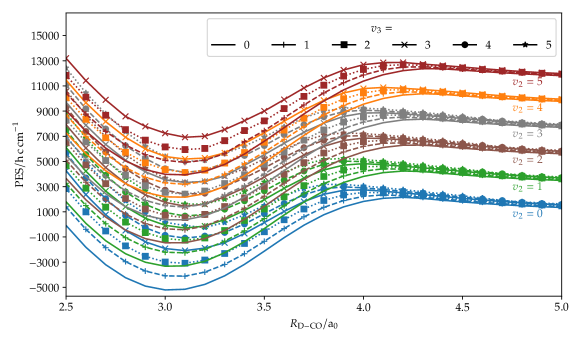
Figure 4: Adiabatic potential energy curves for the CO vibrational problem as a function of D-CO distance $R$ in Jacobi coordinates; see Eq.  (9). The adiabatic curves are assigned DC=O stretch $v_{2}$ and D-C=O rotation $v_{3}$ quantum numbers according to the character of the eigenstates. Note the occurrence of many avoided crossings where the character of the adiabatic states is ambiguous. Further, note that only a selection of curves ($v_{2}\leq 5$ and $v_{3}\leq 5$) is depicted, i.e., there are many more curves in this energy region. For $v_{2}\geq 4$, only curves for $v_{3}\leq 3$ are shown and they should be regarded as qualitative in the interaction region.

Selected adiabatic potential energy curves are shown in Fig.  4. For $R<4\,\mathrm{a_{0}}$, there are many avoided crossings and as such strong couplings between states that have a different $v_{2}$ number. For example, the curve for $v_{2}=3,v_{3}=0$ shows a coupling with $v_{2}=0,v_{3}=5$ and, at small $R$, even with $v_{2}=0,v_{3}=4$. These curves can be used to qualitatively understand the mixing of the zero-order states: Resonance state (0,5,1) has contributions of (2,3,1), (1,4,1) and (0,4,3) (see Table 2). The avoided crossing at $R\approx 3.3\,\mathrm{a_{0}}$ for $v_{2}=5,v_{3}=1$ and $v_{2}=4,v_{3}=3$ explains the mixing of states (0,5,1) and (0,4,3). Although the curve also overlaps with $v_{2}=3,v_{3}=5$, the mixing is less significant because the difference in the character of the two states is larger such that the coupling is reduced. Due to the excitation in $v_{1}$, states (2,3,1) and (1,4,1) mix with (0,5,1) as well.

It would strongly simplify the analysis of the decomposition of the states if the adiabatic states $\left|{\chi_{n}(r,\theta;R)}\right\rangle$ were (quasi-)diabatized such that the character of the states does not change for all considered values of $R$. A projection of the resonance states onto the diabatized states would give a quantitative decomposition in terms of quantum numbers $v_{2}$ and $v_{3}$. However, we were not able to obtain useful diabatic states that have a conserved nodal pattern for all values of $R$; see Section iii in the supplementary material for more details.

IV.5 Product distributions

The experimental and convoluted theoretical KER spectra for resonance states (2,2,2), (0,5,0), (2,3,1) and (1,4,1) are shown in Fig.  5. All theoretical KER spectra without convolution are shown in the supplementary information (Figures iv – xiv). The agreement between the theoretical and the experimental spectra is good. For (0,5,0) the spectrum from the SAG surface agrees better with experiment. Whereas the spectrum from the WKS surface shows a bimodal distribution, both experimental and SAG spectra show a monomodal rotational distribution for $v=0$. This is in accord with the better agreement of the resonance width. For the WKS surface, the width is too small; compare with Table 3. However, for the other three resonances, the WKS surface shows better agreement with the experiment, both in terms of peak positions and intensities. Compared to the experimental results, some, but not all, peaks exhibit a minor shift. This cannot be explained simply by a different asymptotic dissociation energy because there is no consistent trend. Instead, the shifts probably arise because the KER spectra are very sensitive to the shape of the PES, in particular near the transition region.

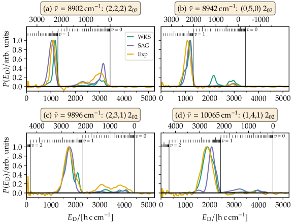
Figure 5: Experimental (Exp) and convoluted theoretical (WKS and SAG) total kinetic energy release spectra $P(E_{\ce{D}})$ and corresponding CO rovibrational product state distributions for the experimentally investigated DCO ($\widetilde{X}$) resonance states. WKSWerner et al. (1995); Keller et al. (1996) and SAGSong, van der Avoird, and Groenenboom (2013) stands for the two employed PES. The vertical lines indicate the maximal available energies $E_{\text{avl}}$ for formation of CO in $v$ = 0, 1 and 2 and the energies of the CO product rotational ($j$) states. The CO rovibrational energies corresponding to the vertical lines are obtained from computations with the WKS PES. The theoretical curves are convoluted with a Gaussian, $\exp[-(E/\sigma)^{2}/2]$, with an arbitrarily chosen width of $\sigma=60\,\mathrm{{h\,c\,}cm^{-1}}$.

To allow for a easier comparison of the theoretical results, we have converted the energetically resolved spectra to distributions resolved rovibrationally by the asymptotic CO fragment (see subsection III.3). Two of the distributions (for resonances (2,3,1) and (0,5,0)) are shown in Fig.  6 (black/darker bars). The rest of the distributions is shown in the supplementary material (Figures xv – xxiv). Except for (0,2,7), all computed resonances have major contributions for $v=1$ (compared to $v=0$) and negligible contributions for $v=2$. As in HCO,Werner et al. (1995); Dixon (1992) the distributions typically are multimodal. Especially the resonances with large initial quantum numbers in $v_{2}$ and $v_{3}$ show a complicated multimodal pattern for a CO stretch quantum number of $v=0$. The multimodal pattern is in agreement with semiclassical estimates used for H2O and HCO.Schinke et al. (1991); Werner et al. (1995); Keller and Schinke (1997)

To evaluate the changes of these distributions during the decay, we projected the part of the initial ($t=0$) resonance that lies in the dissociation region (we chose $R\geq 5\,\mathrm{a_{0}}$) onto the asymptotic rovibrational states; see Eq.  (4). Characteristic examples of such distribution changes are shown as gray/brighter bars in Fig.  6. The relative amount of the initial wavepacket that lies in this asymptotic region ranges from $7\%$ (resonance (0,5,0)) to $33\%$ (resonance (3,2,1)). For most resonances, this ratio lies between $13\%$ and $20\%$. In most cases, the qualitative features of these asymptotic distributions do not change during the dynamics, hence the projection at $t=0$ provides a very reasonable estimate of the rovibrational product distribution, even though the major part (typically more than $80\%$) of the initial wavepacket resides in the interaction region. Some resonances exhibit a shift to higher (lower) $j$ values for $v=0$ ($v=1$).

Only for those resonances that have a small decay width ((0,5,0), (1,3,2), (2,3,0) and (1,4,0); (2,3,1) on the SAG surface), we see larger deviations, see, e.g., resonance (0,5,0) in Fig.  6. A small decay width means a long decay time and as such more time for interference processes etc. which lead to these more significant asymptotic pattern changes. This follows from an investigation of the non-adiabatic coupling elements of the adiabatic, $R$-dependent rovibrational states (see subsection IV.4). It shows that the different states couple with each other even for $R>4.5\,\mathrm{a_{0}}$, especially those with the same quantum number $v_{2}$; compare with Fig.  4 and Section iii in the supplementary material. Further, the stated resonances are those where less than $10\%$ of the initial wavepacket lies in the interaction region (naturally, a small decay width causes a smaller fraction of that resonance in the asymptotic region).

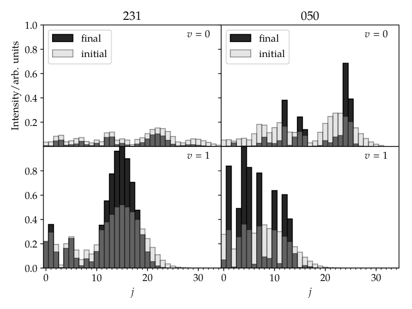
Figure 6: Asymptotic distributions resolved by CO vibration-rotation quantum numbers, for resonances (2,3,1) (left) and (0,5,0) (right) using the WKS PES.Werner et al. (1995); Keller et al. (1996) The upper (lower) panels show the distributions for stretch quantum number $v=0$ ($v=1$) versus different rotational quantum numbers $j$ of the asymptotic CO fragment (bend quantum numbers for the undissociated state). The distributions are scaled such that the maximal value is $1$. The darker bars show the distributions for the final wavepacket, $|{\Psi(t\to\infty)}\rangle$, the brighter bars for the initial wavepacket, $|{\Psi(t=0)}\rangle$, both in the asymptotic region.

IV.6 Decay processes

We now analyze and discuss mechanisms of resonance decay, i.e., the occurrence of IVR during the decay. For that, the coordinate range in $R$ is increased (compare with subsection IV.2) such that the resonance states obtained from filter diagonalization are no longer eigenstates and will spread in $R$ and decay. Note that we analyze here the part of the wavepacket that remains in the interaction region during the decay. A loss in a quantum number during the IVR means that the corresponding energy is moved from the interaction region to the continuum.

Using a polyad model Hamiltonian, the Temps group has already done an IVR analysis.Troellsch and Temps (2001); Renth, Temps, and Tröllsch (2003) During dissociation, the bending motion (quantum number $v_{3}$) turns into rotational motion of the CO fragment (quantum number $j$). Semiclassically, four quanta need to be transferred to the D-C stretch degree of freedom. The C-O stretch quantum number $v_{2}$ remains (approximately) conserved and turns into $v$.

Here, we consider the ab initio Hamiltonian, where an in-depth and quantitative analysis is not possible. As already mentioned in Section I, the assignment in terms of zero-order eigenstates and their vibrational quantum numbers is problematic. This was already visible in Table 2 above, and it becomes even more obvious when analyzing the time-dependent wavefunctions further: Already counting the number of nodes (by plotting $\Re{(\Psi)}$) or counting the number of pronounced lobes (by plotting $|\Psi|^{2}$) can lead to different assignments because the intensities of the lobes vary significantly. In this sense, any assignment should be regarded as approximate, and the IVR mechanism should be regarded as qualitative.

In the following, the assignment is performed based on counting the number of lobes. Qualitatively, we reproduced the assignment from LABEL:\cite[citenum]{\@@bibref{Number}{missing}{}{}}DCO_II_schinke (see Table 2). The assignment was done based on cuts of Jacobi coordinates that have been shifted and rotated such that the first excited adiabatic state retained its orientation for different cut values (see also subsection IV.4). Further, we plotted cuts in Eckart bond coordinates, i.e., coordinates $\{X,Y,\phi\}$, where $X$ ($Y$) is the C-D (C-O) distance and $\phi$ the angle $\sphericalangle(\ce{DCO})$ between the corresponding vectors $\vec{X}$ and $\vec{Y}$. Here, we solely show cuts of the wavefunction in Eckart coordinates, since they provide clearer nodal patterns in the decisive interaction region. Throughout, all cuts are performed along coordinate values that show significant contributions to the wavefunction.

Note that we analyze the wavefunction in the interaction region, that is, we analyzed that part of the wavefunction that remains bound during the studied propagation times. Hence, the following analysis is not directly comparable with the rovibrational product state distributions shown in subsection IV.5. The direct conversion of the bound to the unbound part in the continuum is hard to analyze since it happens over a wide coordinate range and over long propagation times and since the initial wavefunctions already extends into the dissociation region. Indeed, already the initial wavefunctions qualitatively contains all required components in the asymptotic region (see subsection IV.5), although these asymptotic parts typically contribute only 13–20% to the total resonance wavefunction.

IV.6.1 Polyad 5

Cuts of the decay of the (0,3,4) resonance in the plane of C-O stretching (D-C stretching) and D-C-O bending are shown in Eckart bond coordinates in Fig.  7 (Fig.  8). The upper left panel of Fig.  7 shows a part of the initial resonance that can be assigned as $v_{1}=3$ and $v_{3}=4$ (there are four lobes in the C-O distance $Y$ and five lobes in the bending angle $\phi$). Here, the assignment is already ambiguous, because there is no contiguous nodal pattern. However, an inspection of different cuts and in different coordinates (see subsection IV.6) verifies the assignment. The upper left panel of Fig.  8 shows a part of the initial resonance that can clearly be assigned as $v_{{1}}=0$ and $v_{3}=4$. Note that the other zero-order components are typically visible in different coordinate ranges such that there are regions where the different components do not significantly overlap.

A distinctive change in the vibrational structure happens only after the norm of the wavefunction has decreased to $0.15$ or less. A decrease of the norm means a decay of the wavefunction because it entered the region of the CAP. This is also the case for the other resonances studied. Before IVR takes place, there are oscillations between the different zero-order components of the wavefunction, that is, the intensities of the lobes change. This can be seen in the plots shown in the upper two panels of Fig.  7, although the oscillations are typically less intensive.

At propagation times when the norm is below $0.15$, a decrease of the bending quantum number $v_{3}$ from $4$ to $2$ happens; see Fig.  7 and 8. Neither an increase in $v_{1}$ nor a change in $v_{2}$ is visible in the interaction region. This is valid also for other cuts of the wavefunction where other zero-order states show contributions. For the zero-order $411$ contribution to the 034 resonance, there is an additional decrease of $v_{1}$ to $2$. The oscillations of the different zero-order states, the approximate conversion of quantum number $v_{2}$ and the decay of $v_{3}$ are all in agreement with the analysis done by a polyadic model Hamiltonian.Troellsch and Temps (2001); Renth, Temps, and Tröllsch (2003)

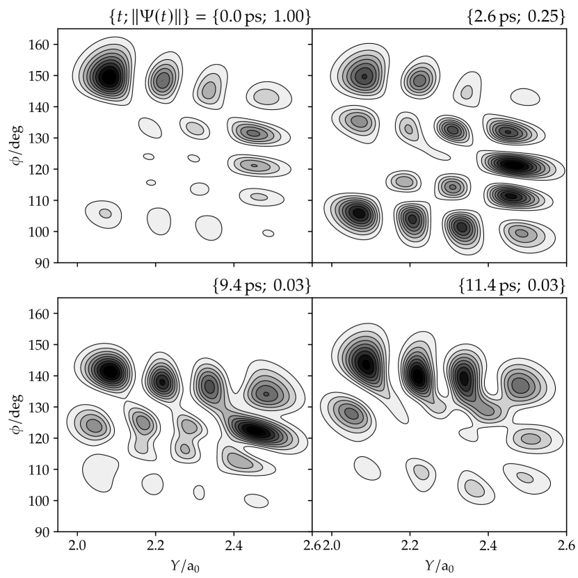
Figure 7: Contour values of $|\Psi(X,Y,\phi;t)|^{2}$ at $X=2.2\,\mathrm{a_{0}}$ and different times, for the (0,3,4) resonance. $X$ is the D-C distance, $Y$ the C3O distance and $\phi$ the D-C=O bending angle in Eckart bond coordinates. For each panel, the shown function is normalized to have the maximal value of $1$. For a comparison of the relative intensity, see the norm values in the panel captions.

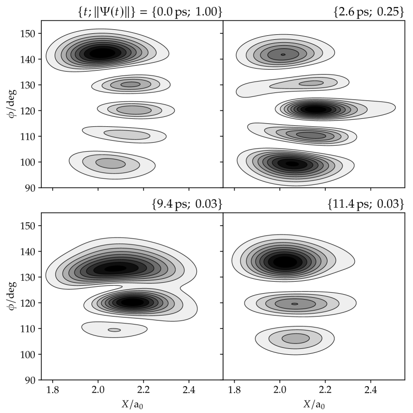
Figure 8: Same as Fig.  7 but showing cuts of $|\Psi(X,Y,\phi;t)|^{2}$ at $Y=2.53\,\mathrm{a_{0}}$. $X$ is the D-C distance, $Y$ the C3O distance and $\phi$ the D-C=O bending angle in Eckart bond coordinates.

For the resonances (0,4,2), (2,2,2), (0,5,0), (1,3,2), (2,3,0), (1,4,0) (polyad 5) and (0,4,3) (polyad 5.5), only minor oscillations of the lobes occur. No IVR is visible and the oscillations are much less pronounced than that shown in the upper panels of Fig.  7 for (0,3,4). To some extent, this can be explained by the small decay rate of the resonances. Except for (0,4,3) (polyad 5.5), they all have a decay width of $\Gamma\leq 0.32\,\mathrm{cm^{-1}}$. In polyad 5.5, resonance (0,4,3) has the second smallest value of $\Gamma$. A small reaction rate is correlated with a hindered IVR.Renth, Temps, and Tröllsch (2003) However, resonance (0,5,1), the resonance with the smallest value of $\Gamma$ ($0.64\,\mathrm{cm^{-1}}$) in polyad 5.5, does show a decay mechanism (see subsubsection IV.6.2) but also lies higher in energy and has an evenly spread-out distribution of four zero-order components such that the coupling to other states may be larger; see also below.

To show how insignificant the temporal change in wavefunction structure can be, consider the cut of the (0,5,0) resonance shown in Fig.  9. Even after propagating for 175 ps and after decay of the norm to a value of $0.11$, the structure does not change. For checking our results, we have propagated the (0,5,0) state using smaller coordinate ranges and a higher propagator accuracy with a standard DVR code (without DP) until 300 ps, where the norm has dropped down to a value of $0.02$. Even then, no significant change in the structure of the wavefunction is visible. Additionally, our DP-DVR results are confirmed by this conventional DVR run.

For a polyadic model Hamiltonian, Temps et al. studied the decay of a pure (0,5,0) state.Renth, Temps, and Tröllsch (2003) The state turned, among others, into (1,4,0) and (2,3,0) within less than $0.5\,\mathrm{ps}$. Here, already the initial resonance state consists of these components (not seen in the cuts shown in Fig.  9); see Table 2. Hence, the initial state already has all main zero-order components needed for the IVR to happen. This explains the small oscillations in the nodal pattern.

This further means that the zero-order states included in the initial resonance states are strongly coupled whereas they couple weakly to other states. The strong coupling of the states within one polyad is stressed in LABEL:\cite[citenum]{\@@bibref{Number}{missing}{}{}}DCO_I_schinke. Indeed, resonances (0,4,2), (2,2,2) and (1,3,2) consist of the corresponding zero-order states and so do resonances (0,5,0), (1,4,0) and (2,3,0); see Table 2. In contrast, resonance (0,3,4) shows an IVR. However, its decay rate is much larger and the resonance has components of (2,2,2) but also of the different zero-order states (4,1,1) and (1,2,4). The strong coupling between states $\{(0,4,2),(2,2,2),(1,3,2)\}$ and $\{(0,5,0),(1,5,0),(2,3,0)\}$ is in agreement with the parameters from the polyadic model Hamiltonian.Troellsch and Temps (2001)

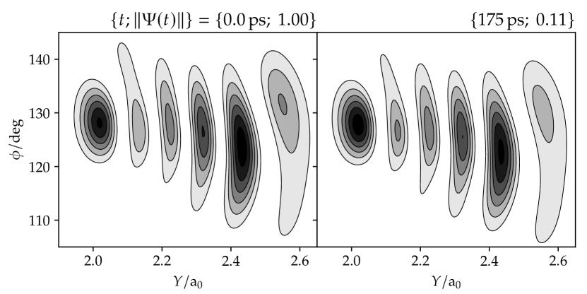
Figure 9: Same as Fig.  7 but showing cuts of $|\Psi(X,Y,\phi;t)|^{2}$ at $X=2.15\,\mathrm{a_{0}}$ for the (0,5,0) resonance.

Considering the insignificant changes of the wavefunction within the interaction region, it may seem counterintuitive that for a subset of these states the asymptotic rovibrational distributions of the CO fragment do change significantly in time. However, as pointed out in subsection IV.5, the rovibrational states still couple outside the typical interaction region where $R<4.5\,\mathrm{a_{0}}$, such that the dynamics in the asymptote and in the interaction regions are, to first order, not directly related. In fact, from Fig.  4, it may be argued that the distribution of the adiabatic states on the energy axis, and thus also their couplings, strongly change between $R<4.0\,\mathrm{a_{0}}$ and $R>4.0\,\mathrm{a_{0}}$, supporting different dynamical behaviors.

As a side remark: On the SAG surface, resonance (0,5,0) does show an IVR with an increase in $v_{3}$ to $1$ (with intermediate numbers up to $v_{3}=3$) and a decrease in $v_{2}$ up to $v_{2}=2$. However, the character of this resonance state also differs from the state computed on the WKS surface. Most importantly, the initial state already has some contributions of $v_{3}=1$ which the state on the WKS surface does not have (see Table 2). Note that, in this case, $\Gamma$ is larger and, like the KER, closer to the experimental value on the SAG surface. Resonances with excitations in both $v_{2}$ and $v_{3}$ exhibit larger decay rates than those with excitations only in $v_{3}$.Keller et al. (1997)

IV.6.2 Polyad 5.5

In polyad 5.5, resonance (0,2,7) decays rapidly with a decrease in $v_{2}$. However, it has a strong contribution at the linear geometry. Due to the neglect of Renner-Teller coupling in this simulation and since resonance states with high bending motion are experimentally hard to measure, we have not analyzed this state further in the present study.

As already mentioned in subsubsection IV.6.1, resonance (0,4,3) shows only minor oscillations between the zero-order components of the initial state. Resonance (2,2,3) shows a decrease in $v_{3}$ from $3$ to $\{1,0\}$ (both $1$ and $0$) and an increase in $v_{2}$ from $4$ to $5$. However, due to a component of $v_{3}=5$, it shows also contributions at linear geometry and the results have to be taken with caution. As for the previous resonances where a clear IVR takes place, (0,5,1) shows a decrease in $v_{3}$ whereas $v_{2}$ remains mostly conserved. Likewise, 133 decays to $v_{3}=\{2,1\}$ and the zero-order (0,5,1) state initially contributing by $\sim~{}21\%$ (Table 2) gets more populated.

A decrease in $v_{3}$ to $0$ while the other quantum numbers are approximately conserved is clearly seen also in state (2,3,1), see Fig.  10 and Fig.  11. Both cuts in $Y$ and $X$ show a decrease in $v_{3}$ whereas the $v_{2}=3$ and $v_{1}=2$ components are constant. At $26\,\mathrm{ps}$, the cut shown in $Y$ (right panel in Fig.  11) is more difficult to analyze because contributions from other zero-order states become more visible.

The corresponding state on the SAG surface shows no significant IVR. There, the state has similar zero-order components except for a reduced $v_{1}=2$ component. This decreases the decay width which is smaller, compared to experiment; see Table 3). The hindered IVR due to the smaller decay width ($\Gamma=0.36\,\mathrm{cm^{-1}}$) is in agreement with the discussion in subsubsection IV.6.1.

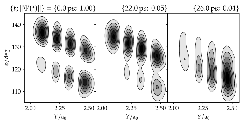
Figure 10: Same as Fig.  7 but showing cuts of $|\Psi(X,Y,\phi;t)|^{2}$ at $X=1.85\,\mathrm{a_{0}}$ for the (2,3,1) resonance.

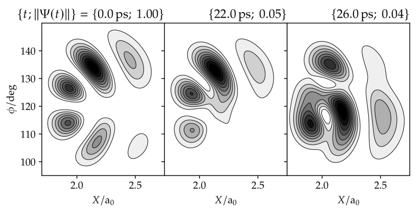
Figure 11: Same as Fig.  7 but showing cuts of $|\Psi(X,Y,\phi;t)|^{2}$ at $Y=2.5\,\mathrm{a_{0}}$ for the (2,3,1) resonance.

As (2,3,1), state (1,4,1) decays in $v_{3}$. Here, the $v_{2}=5$ component (see Table 2) becomes more pronounced. The contribution of the (4,2,0) zero-order state shows a decay from $v_{1}=4$ to $v_{1}=1$, see Fig.  12. There, the wavefunction looks like it has increased in $v_{3}$ but an inspection of the phase cannot clearly confirm this.

State (1,4,1) computed on the SAG surface shows a similar initial state (with a reduced component of the (2,3,1) state) and a similar decay mechanism. There, $\Gamma$ is lower ($0.85\,\mathrm{cm^{-1}}$ compared to the experimental value of $6\,\mathrm{cm^{-1}}$; see Table 3), but not too low for IVR, compared to the resonances that show no pronounced IVR.

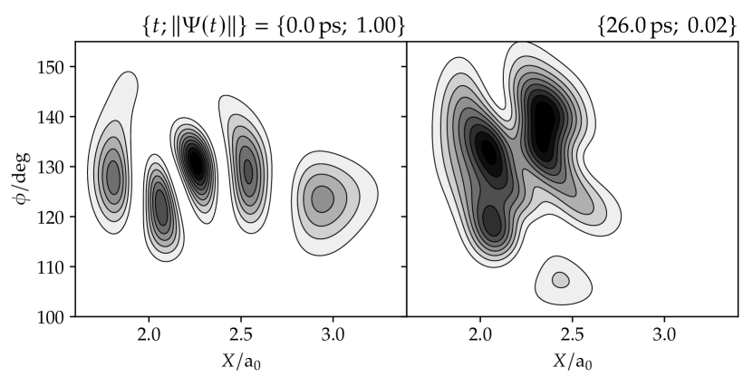
Figure 12: Same as Fig.  7 but showing cuts of $|\Psi(X,Y,\phi;t)|^{2}$ at $Y=2.09\,\mathrm{a_{0}}$ for the (1,4,1) resonance.

A sequential decay from $v_{1}=3$ via $v_{1}=2$ to $v_{1}=\{1,0\}$ in conjunction with a decay of $v_{3}=1$ to $v_{3}=0$ can be observed for resonance (3,2,1). Again, $v_{2}$ remains conserved. Note that this resonance in polyad 5.5 has the highest D-C stretch excitation. Due to the large decay width of $\Gamma=17\,\mathrm{cm^{-1}}$, the IVR begins quickly and there are intermediate states with contributions from many zero-order states that are hard to analyze. Note that this state has some contributions of $v_{3}=5$ and, due to this high excitation in the bending mode, contributions at linear geometries. However, they are less pronounced than for the other states with similar contributions.

While a decrease in bending quantum number $v_{3}$ can be seen in all resonances where a clear IVR occurs, a decrease in D-C stretch quantum number $v_{1}$ can only be seen for $v_{1}>2$, namely in states (3,2,1), (1,4,1) and (0,3,4) where the latter two have zero-order states with $v_{1}=4$.

V Conclusions

To summarize, we have employed our newly developed dynamically pruned DVR (DP-DVR) for computing resonance states in DCO of polyads $5$ and $5.5$ using filter diagonalization and for subsequential propagation to analyze their decay mechanisms. For selected resonances, the kinetic energy release (KER) spectra were compared to experimental results obtained from velocity-map images.

For this challenging test case where the wavefunction has to be propagated in the asymptotic region for up to 180 picoseconds, DP-DVR works well and the computed resonance energies and widths show good agreement with results from the literature. The computed KER spectra are in good agreement with the experimental spectra. Two PES have been compared. For many states, the WKS surfaceWerner et al. (1995) gives slightly better results than the SAG surface.Song, van der Avoird, and Groenenboom (2013) Since no PES was constructed with this particular application in mind (decay dynamics of energetically high-lying resonances far out into the asymptote), no quantitative agreement between theoretical and experimental results can be expected. Also, the importance of including $J>0$ and Renner-Teller couplings to higher electronic states at linear geometries still has to be elucidated.

The rovibrational distribution of the asymptotic CO states shows major contributions only for C3O stretch quantum numbers $v=0$ and $1$. The distribution in the CO rotational quantum number $j$ is multimodal. For states with larger decay widths of $\Gamma>0.6\,\mathrm{cm^{-1}}$, the initial state already shows the qualitatively correct shape of the distributions. Due to a coupling of the rovibrational states even in the near-asymptotic region, states with smaller decay rates show qualitatively different distributions after long propagation times.

Analyses of the decay processes confirm the results from a polyad model Hamiltonian.Troellsch and Temps (2001, 2001) For the studied resonance states, the $v_{2}$ quantum number typically is a conserved quantity while the wavefunction part in the interaction region shows a decrease in quantum number $v_{3}$. For high D-CO stretch excitations with corresponding quantum number $v_{2}>2$, a decay in this quantum number is possible as well. In contrast to the polyad model, all resonance states show significant mixing of zero-order states.

Some zero-order states, in particular in polyad $5$, show very strong coupling with each other. Almost all zero-order components needed for an IVR are already contained in the initial resonance state and, for these states, no appearance or disappearance of additional zero-order components can be observed.

The qualitative agreements between a polyad model and full quantum dynamics confirm that there are analyzable residues of orderly IVR mechanisms present in the strongly anharmonic DCO system. However, not surprisingly, our full quantum dynamics also indicate where and how a mechanistic understanding has to transcend a zero-order model picture.

Supplementary material

See supplementary material for plots of the PES, the propagation times, details on the diabatization and the asymptotic distributions of all resonance states.