The Description Length of Deep Learning Models

Abstract

Solomonoff’s general theory of inference (Solomonoff, 1964) and the Minimum Description Length principle (Grünwald, 2007, Rissanen, 2007) formalize Occam’s razor, and hold that a good model of data is a model that is good at losslessly compressing the data, including the cost of describing the model itself. Deep neural networks might seem to go against this principle given the large number of parameters to be encoded.

We demonstrate experimentally the ability of deep neural networks to compress the training data even when accounting for parameter encoding. The compression viewpoint originally motivated the use of variational methods in neural networks (Hinton and Van Camp, 1993, Schmidhuber, 1997). Unexpectedly, we found that these variational methods provide surprisingly poor compression bounds, despite being explicitly built to minimize such bounds. This might explain the relatively poor practical performance of variational methods in deep learning. On the other hand, simple incremental encoding methods yield excellent compression values on deep networks, vindicating Solomonoff’s approach.

1 Introduction

Deep learning has achieved remarkable results in many different areas (LeCun et al., 2015). Still, the ability of deep models not to overfit despite their large number of parameters is not well understood. To quantify the complexity of these models in light of their generalization ability, several metrics beyond parameter-counting have been measured, such as the number of degrees of freedom of models (Gao and Jojic, 2016), or their intrinsic dimension (Li et al., 2018). These works concluded that deep learning models are significantly simpler than their numbers of parameters might suggest.

In information theory and Minimum Description Length (MDL), learning a good model of the data is recast as using the model to losslessly transmit the data in as few bits as possible. More complex models will compress the data more, but the model must be transmitted as well. The overall codelength can be understood as a combination of quality-of-fit of the model (compressed data length), together with the cost of encoding (transmitting) the model itself. For neural networks, the MDL viewpoint goes back as far as (Hinton and Van Camp, 1993), which used a variational technique to estimate the joint compressed length of data and parameters in a neural network model.

Compression is strongly related to generalization and practical performance. Standard sample complexity bounds (VC-dimension, PAC-Bayes…) are related to the compressed length of the data in a model, and any compression scheme leads to generalization bounds (Blum and Langford, 2003). Specifically for deep learning, (Arora et al., 2018) showed that compression leads to generalization bounds (see also (Dziugaite and Roy, 2017)). Several other deep learning methods have been inspired by information theory and the compression viewpoint. In unsupervised learning, autoencoders and especially variational autoencoders (Kingma and Welling, 2013) are compression methods of the data (Ollivier, 2014). In supervised learning, the information bottleneck method studies how the hidden representations in a neural network compress the inputs while preserving the mutual information between inputs and outputs (Tishby and Zaslavsky, 2015, Shwartz-Ziv and Tishby, 2017, Achille and Soatto, 2017).

MDL is based on Occam’s razor, and on Chaitin’s hypothesis that “comprehension is compression” (Chaitin, 2007): any regularity in the data can be exploited both to compress it and to make predictions. This is ultimately rooted in Solomonoff’s general theory of inference (Solomonoff, 1964) (see also, e.g., (Hutter, 2007, Schmidhuber, 1997)), whose principle is to favor models that correspond to the “shortest program” to produce the training data, based on its Kolmogorov complexity (Li and Vitányi, 2008). If no structure is present in the data, no compression to a shorter program is possible.

The problem of overfitting fake labels is a nice illustration: convolutional neural networks commonly used for image classification are able to reach $100\%$ accuracy on random labels on the train set (Zhang et al., 2017). However, measuring the associated compression bound (Fig. 1) immediately reveals that these models do not compress fake labels (and indeed, theoretically, they cannot, see Appendix A), that no information is present in the model parameters, and that no learning has occurred.

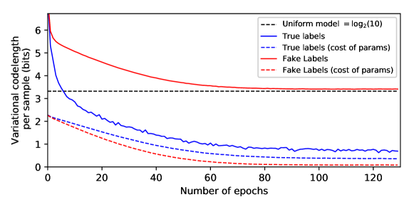
Figure 1: Fake labels cannot be compressed Measuring codelength while training a deep model on MNIST with true and fake labels. The model is an MLP with 3 hidden layers of size 200, with RELU units. With ordinary SGD training, the model is able to overfit random labels. The plot shows the effect of using variational learning instead, and reports the variational objective (encoding cost of the training data, see Section 3.3), on true and fake labels. We also isolated the contribution from parameter encoding in the total loss (KL term in (3.2)). With true labels, the encoding cost is below the uniform encoding, and half of the description length is information contained in the weights. With fake labels, on the contrary, the encoding cost converges to a uniform random model, with no information contained in the weights: there is no mutual information between inputs and outputs.

In this work we explicitly measure how much current deep models actually compress data. (We introduce no new architectures or learning procedures.) As seen above, this may clarify several issues around generalization and measures of model complexity. Our contributions are:

• We show that the traditional method to estimate MDL codelengths in deep learning, variational inference (Hinton and Van Camp, 1993), yields surprisingly inefficient codelengths for deep models, despite explicitly minimizing this criterion. This might explain why variational inference as a regularization method often does not reach optimal test performance.

• We introduce new practical ways to compute tight compression bounds in deep learning models, based on the MDL toolbox (Grünwald, 2007, Rissanen, 2007). We show that prequential coding on top of standard learning, yields much better codelengths than variational inference, correlating better with test set performance. Thus, despite their many parameters, deep learning models do compress the data well, even when accounting for the cost of describing the model.

2 Probabilistic Models, Compression, and Information Theory

Imagine that Alice wants to efficiently transmit some information to Bob. Alice has a dataset $\mathcal{D}=\{(x_{1},y_{1}),...,(x_{n},y_{n})\}$ where $x_{1},...,x_{n}$ are some inputs and $y_{1},...,y_{n}$ some labels. We do not assume that these data come from a “true” probability distribution. Bob also has the data $x_{1},...,x_{n}$, but he does not have the labels. This describes a supervised learning situation in which the inputs $x$ may be publicly available, and a prediction of the labels $y$ is needed. How can deep learning models help with data encoding? One key problem is that Bob does not necessarily know the precise, trained model that Alice is using. So some explicit or implicit transmission of the model itself is required.

We study, in turn, various methods to encode the labels $y$, with or without a deep learning model. Encoding the labels knowing the inputs is equivalent to estimating their mutual information (Section 2.4); this is distinct from the problem of practical network compression (Section 3.2) or from using neural networks for lossy data compression. Our running example will be image classification on the MNIST (LeCun et al., 1998) and CIFAR10 (Krizhevsky, 2009) datasets.

2.1 Definitions and notation

Let $\mathcal{X}$ be the input space and $\mathcal{Y}$ the output (label) space. In this work, we only consider classification tasks, so $\mathcal{Y}=\{1,...,K\}$. The dataset is $\mathcal{D}\mathrel{\mathop{:}}=\{(x_{1},y_{1}),...,(y_{n},x_{n})\}$. Denote $x_{k:l}\mathrel{\mathop{:}}=(x_{k},x_{k+1},...,x_{l-1},x_{l})$. We define a model for the supervised learning problem as a conditional probability distribution $p(y|x)$, namely, a function such that for each $x\in\mathcal{X}$, $\sum_{y\in\mathcal{Y}}p(y|x)=1$. A model class, or architecture, is a set of models depending on some parameter $\theta$: $\mathcal{M}=\{p_{\theta},\theta\in\Theta\}$. The Kullback–Leibler divergence between two distributions is $\operatorname{{\mathrm{KL}}}(\mu\|\nu)=\mathbb{E}_{X\sim\mu}[\log_{2}\frac{\mu(x)}{\nu(x)}]$.

2.2 Models and codelengths

We recall a basic result of compression theory (Shannon, 1948).

Proposition 1 (Shannon–Huffman code).

Suppose that Alice and Bob have agreed in advance on a model $p$, and both know the inputs $x_{1:n}$. Then there exists a code to transmit the labels $y_{1:n}$ losslessly with codelength (up to at most one bit on the whole sequence)

$$L_{p}(y_{1:n}|x_{1:n})=-\sum_{i=1}^{n}\log_{2}p(y_{i}|x_{i})$$ (2.1)

This bound is known to be optimal if the data are independent and coming from the model $p$ (Mackay, 2003). The one additional bit in the Shannon–Huffman code is incurred only once for the whole dataset (Mackay, 2003). With large datasets this is negligible. Thus, from now on we will systematically omit the $+1$ as well as admit non-integer codelengths (Grünwald, 2007). We will use the terms codelength or compression bound interchangeably.

This bound is exactly the categorical cross-entropy loss evaluated on the model $p$. Hence, trying to minimize the description length of the outputs over the parameters of a model class is equivalent to minimizing the usual classification loss.

Here we do not consider the practical implementation of compression algorithms: we only care about the theoretical bit length of their associated encodings. We are interested in measuring the amount of information contained in the data, the mutual information between input and output, and how it is captured by the model. Thus, we will directly work with codelength functions.

An obvious limitation of the bound (2.1) is that Alice and Bob both have to know the model $p$ in advance. This is problematic if the model must be learned from the data.

2.3 Uniform encoding

The uniform distribution $p_{\mathrm{unif}}(y|x)=\frac{1}{K}$ over the $K$ classes does not require any learning from the data, thus no additional information has to be transmitted. Using $p_{\mathrm{unif}}(y|x)$ (2.1) yields a codelength

$$L^{\mathrm{unif}}(y_{1:n}|x_{1:n})=n\log_{2}K$$ (2.2)

This uniform encoding will be a sanity check against which to compare the other encodings in this text. For MNIST, the uniform encoding cost is $60000\times\log_{2}10=199\operatorname{kbits}$. For CIFAR, the uniform encoding cost is $50000\times\log_{2}10=166\operatorname{kbits}$.

2.4 Mutual information between inputs and outputs

Intuitively, the only way to beat a trivial encoding of the outputs is to use the mutual information (in a loose sense) between the inputs and outputs.

This can be formalized as follows. Assume that the inputs and outputs follow a “true” joint distribution $q(x,y)$. Then any transmission method with codelength $L$ satisfies (Mackay, 2003)

$$\mathbb{E}_{q}[L(y|x)]\geq H(y|x)$$ (2.3)

Therefore, the gain (per data point) between the codelength $L$ and the trivial codelength $H(y)$ is

$$H(y)-\mathbb{E}_{q}[L(y|x)]\leq H(y)-H(y|x)=I(y;x)$$ (2.4)

the mutual information between inputs and outputs (Mackay, 2003).

Thus, the gain of any codelength compared to the uniform code is limited by the amount of mutual information between input and output. (This bound is reached with the true model $q(y|x)$.) Any successful compression of the labels is, at the same time, a direct estimation of the mutual information between input and output. The latter is the central quantity in the Information Bottleneck approach to deep learning models (Shwartz-Ziv and Tishby, 2017).

Note that this still makes sense without assuming a true underlying probabilistic model, by replacing the mutual information $H(y)-H(y|x)$ with the “absolute” mutual information $K(y)-K(y|x)$ based on Kolmogorov complexity $K$ (Li and Vitányi, 2008).

3 Compression Bounds via Deep Learning

Table 1: Compression bounds via Deep Learning. Compression bounds given by different codes on two datasets, MNIST and CIFAR10. The Codelength is the number of bits necessary to send the labels to someone who already has the inputs. This codelength includes the description length of the model. The compression ratio for a given code is the ratio between its codelength and the codelength of the uniform code. The test accuracy of a model is the accuracy of its predictions on the test set. For 2-part and network compression codes, we report results from (Han et al., 2015a) and (Xu et al., 2017), and for the intrinsic dimension code, results from (Li et al., 2018). The values in the table for these codelengths and compression ratio are lower bounds, only taking into account the codelength of the weights, and not the codelength of the data encoded with the model (the final loss is not always available in these publications). For variational and prequential codes, we selected the model and hyperparameters providing the best compression bound.

Code	mnist			cifar10
	Codelength	Comp.	Test	Codelength	Comp.	Test
	($\operatorname{kbits}$)	Ratio	Acc	($\operatorname{kbits}$)	Ratio	Acc
Uniform	199	1.	10%	166	1.	10%
float32 2-part	$>8.6\mathrm{Mb}$	$>45.$	98.4%	$>428\mathrm{Mb}$	$>2500.$	92.9%
Network compr.	$>400$	$>2.$	98.4%	$>14\mathrm{Mb}$	$>83.$	93.3%
Intrinsic dim.	$>9.28$	$>0.05$	90%	$>92,8$	$>0.56$	70%
Variational	22.2	0.11	98.2%	89.0	0.54	66,5%
Prequential	4.10	0.02	99.5%	45.3	0.27	93.3%

Various compression methods from the MDL toolbox can be used on deep learning models. (Note that a given model can be stored or encoded in several ways, some of which may have large codelengths. A good model in the MDL sense is one that admits at least one good encoding.)

3.1 Two-Part Encodings

Alice and Bob can first agree on a model class (such as “neural networks with two layers and 1,000 neurons per layer”). However, Bob does not have access to the labels, so Bob cannot train the parameters of the model. Therefore, if Alice wants to use such a parametric model, the parameters themselves have to be transmitted. Such codings in which Alice first transmits the parameters of a model, then encodes the data using this parameter, have been called two-part codes (Grünwald, 2007).

Definition 1 (Two-part codes).

Assume that Alice and Bob have first agreed on a model class $(p_{\theta})_{\theta\in\Theta}$. Let $L_{\mathrm{param}}(\theta)$ be any encoding scheme for parameters $\theta\in\Theta$. Let $\theta^{\ast}$ be any parameter. The corresponding two-part codelength is

$$L^{\mathrm{2\text{-part}}}_{\theta^{\ast}}(y_{1:n}|x_{1:n})\mathrel{\mathop{:}}=L_{\mathrm{param}}(\theta^{\ast})+L_{p_{\theta^{\ast}}}(y_{1:n}|x_{1:n})=L_{\mathrm{param}}(\theta^{\ast})-\sum_{i=1}^{n}\log_{2}p_{\theta^{\ast}}(y_{i}|x_{i})$$ (3.1)

An obvious possible code $L_{\mathrm{param}}$ for $\theta$ is the standard float32 binary encoding for $\theta$, for which $L_{\mathrm{param}}(\theta)=32\dim(\theta)$. In deep learning, two-part codes are widely inefficient and much worse than the uniform encoding (Graves, 2011). For a model with 1 million parameters, the two-part code with float32 binary encoding will amount to $32\operatorname{Mbits}$, or 200 times the uniform encoding on CIFAR10.

3.2 Network Compression

The practical encoding of trained models is a well-developed research topic, e.g., for use on small devices such as cell phones. Such encodings can be seen as two-part codes using a clever code for $\theta$ instead of encoding every parameter on $32$ bits. Possible strategies include training a student layer to approximate a well-trained network (Ba and Caruana, 2014, Romero et al., 2015), or pipelines involving retraining, pruning, and quantization of the model weights (Han et al., 2015a, b, Simonyan and Zisserman, 2014, Louizos et al., 2017, See et al., 2016, Ullrich et al., 2017).

Still, the resulting codelengths (for compressing the labels given the data) are way above the uniform compression bound for image classification (Table 1).

Another scheme for network compression, less used in practice but very informative, is to sample a random low-dimensional affine subspace in parameter space and to optimize in this subspace (Li et al., 2018). The number of parameters is thus reduced to the dimension of the subspace and we can use the associated two-part encoding. (The random subspace can be transmitted via a pseudorandom seed.) Our methodology to derive compression bounds from (Li et al., 2018) is detailed in Appendix B.

3.3 Variational and Bayesian Codes

Another strategy for encoding weights with a limited precision is to represent these weights by random variables: the uncertainty on $\theta$ represents the precision with which $\theta$ is transmitted. The variational code turns this into an explicit encoding scheme, thanks to the bits-back argument (Honkela and Valpola, 2004). Initially a way to compute codelength bounds with neural networks (Hinton and Van Camp, 1993), this is now often seen as a regularization technique (Blundell et al., 2015). This method yields the following codelength.

Definition 2 (Variational code).

Assume that Alice and Bob have agreed on a model class $(p_{\theta})_{\theta\in\Theta}$ and a prior $\alpha$ over $\Theta$. Then for any distribution $\beta$ over $\Theta$, there exists an encoding with codelength

$$L^{\mathrm{var}}_{\beta}(y_{1:n}|x_{1:n})=\operatorname{{\mathrm{KL}}}\left(\beta\|\alpha\right)+\mathbb{E}_{\theta\sim\beta}\big{[}L_{p_{\theta}}(y_{1:n}|x_{1:n})\big{]}=\operatorname{{\mathrm{KL}}}\left(\beta\|\alpha\right)-\mathbb{E}_{\theta\sim\beta}\bigg{[}\sum_{i=1}^{n}\log_{2}p_{\theta}(y_{i}|x_{i})\bigg{]}$$ (3.2)

This can be minimized over $\beta$, by choosing a parametric model class $(\beta_{\phi})_{\phi\in\Phi}$, and minimizing (3.2) over $\phi$. A common model class for $\beta$ is the set of multivariate Gaussian distributions $\{\mathcal{N}(\mu,\Sigma),\mu\in\mathbb{R}^{d},\Sigma\;\text{ diagonal}\}$, and $\mu$ and $\Sigma$ can be optimized with a stochastic gradient descent algorithm (Graves, 2011, Kucukelbir et al., 2017). $\Sigma$ can be interpreted as the precision with which the parameters are encoded.

The variational bound $L^{\mathrm{var}}_{\beta}$ is an upper bound for the Bayesian description length bound of the Bayesian model $p_{\theta}$ with parameter $\theta$ and prior $\alpha$. Considering the Bayesian distribution of $y$,

$$p_{\mathrm{Bayes}}(y_{1:n}|x_{1:n})=\int_{\theta\in\Theta}p_{\theta}(y_{1:n}|x_{1:n})\alpha(\theta)d\theta,$$ (3.3)

then Proposition 1 provides an associated code via (2.1) with model $p_{\mathrm{Bayes}}$: $L^{\mathrm{Bayes}}(y_{1:n}|x_{1:n})=-\log_{2}p_{\mathrm{Bayes}}(y_{1:n}|x_{1:n})$ Then, for any $\beta$ we have (Graves, 2011)

$$L^{\mathrm{var}}_{\beta}(y_{1:n}|x_{1:n})\geq L^{\mathrm{Bayes}}(y_{1:n}|x_{1:n})$$ (3.4)

with equality if and only if $\beta$ is equal to the Bayesian posterior $p_{\mathrm{Bayes}}(\theta|x_{1:n},y_{1:n})$. Variational methods can be used as approximate Bayesian inference for intractable Bayesian posteriors.

We computed practical compression bounds with variational methods on MNIST and CIFAR10. Neural networks that give the best variational compression bounds appear to be smaller than networks trained the usual way. We tested various fully connected networks and convolutional networks (Appendix C): the models that gave the best variational compression bounds were small LeNet-like networks. To test the link between compression and test accuracy, in Table 1 we report the best model based on compression, not test accuracy. This results in a drop of test accuracy with respect to other settings.

On MNIST, this provides a codelength of the labels (knowing the inputs) of $24.1\operatorname{kbits}$, i.e., a compression ratio of $0.12$. The corresponding model achieved $95.5\%$ accuracy on the test set.

On CIFAR, we obtained a codelength of $89.0\operatorname{kbits}$, i.e., a compression ratio of $0.54$. The corresponding model achieved $61.6\%$ classification accuracy on the test set.

We can make two observations. First, choosing the model class which minimizes variational codelength selects smaller deep learning models than would cross-validation. Second, the model with best variational codelength has low classification accuracy on the test set on MNIST and CIFAR, compared to models trained in a non-variational way. This aligns with a common criticism of Bayesian methods as too conservative for model selection compared with cross-validation (Rissanen et al., 1992, Foster and George, 1994, Barron and Yang, 1999, Grünwald, 2007).

3.4 Prequential or Online Code

The next coding procedure shows that deep neural models which generalize well also compress well.

The prequential (or online) code is a way to encode both the model and the labels without directly encoding the weights, based on the prequential approach to statistics (Dawid, 1984), by using prediction strategies. Intuitively, a model with default values is used to encode the first few data; then the model is trained on these few encoded data; this partially trained model is used to encode the next data; then the model is retrained on all data encoded so far; and so on.

Precisely, we call $p$ a prediction strategy for predicting the labels in $\mathcal{Y}$ knowing the inputs in $\mathcal{X}$ if for all $k$, $p(y_{k+1}|x_{1:k+1},y_{1:k})$ is a conditional model; namely, any strategy for predicting the $k+1$- label after already having seen $k$ input-output pairs. In particular, such a model may learn from the first $k$ data samples. Any prediction strategy $p$ defines a model on the whole dataset:

$$p^{\mathrm{preq}}(y_{1:n}|x_{1:n})=p(y_{1}|x_{1})\cdot p(y_{2}|x_{1:2},y_{1})\cdot\ldots\cdot p(y_{n}|x_{1:n},y_{1:n-1})$$ (3.5)

Let $(p_{\theta})_{\theta\in\Theta}$ be a deep learning model. We assume that we have a learning algorithm which computes, from any number of data samples $(x_{1:k},y_{1:k})$, a trained parameter vector $\hat{\theta}(x_{1:k},y_{1:k})$. Then the data is encoded in an incremental way: at each step $k$, $\hat{\theta}(x_{1:k},y_{1:k})$ is used to predict $y_{k+1}$.

In practice, the learning procedure $\hat{\theta}$ may only reset and retrain the network at certain timesteps. We choose timesteps $1=t_{0}<t_{1}<...<t_{S}=n$, and we encode the data by blocks, always using the model learned from the already transmitted data (Algorithm 2 in Appendix D). A uniform encoding is used for the first few points. (Even though the encoding procedure is called “online”, it does not mean that only the most recent sample is used to update the parameter $\hat{\theta}$: the optimization procedure $\hat{\theta}$ can be any predefined technique using all the previous samples $(x_{1:k},y_{1:k})$, only requiring that the algorithm has an explicit stopping criterion.) This yields the following description length:

Definition 3 (Prequential code).

Given a model $p_{\theta}$, a learning algorithm $\hat{\theta}(x_{1:k},y_{1:k})$, and retraining timesteps $1=t_{0}<t_{1}<...<t_{S}=n$, the prequential codelength is

$$L^{\mathrm{preq}}(y_{1:n}|x_{1:n})=t_{1}\log_{2}K+\sum_{s=0}^{S-1}-\log_{2}p_{\hat{\theta}_{t_{s}}}(y_{t_{s}+1:t_{s+1}}|x_{t_{s}+1:t_{s+1}})$$ (3.6)

where for each $s$, $\hat{\theta}_{t_{s}}=\hat{\theta}(x_{1:t_{s}},y_{1:t_{s}})$ is the parameter learned on data samples $1$ to $t_{s}$.

The model parameters are never encoded explicitly in this method. The difference between the prequential codelength $L^{\mathrm{preq}}(y_{1:n}|x_{1:n})$ and the log-loss $\sum_{t=1}^{n}-\log_{2}p_{\hat{\theta}_{t_{K}}}(y_{t}|x_{t})$ of the final trained model, can be interpreted as the amount of information that the trained parameters contain about the data contained: the former is the data codelength if Bob does not know the parameters, while the latter is the codelength of the same data knowing the parameters.

Prequential codes depend on the performance of the underlying training algorithm, and take advantage of the model’s generalization ability from the previous data to the next. In particular, the model training should yield good generalization performance from data $[1;t_{s}]$ to data $[t_{s}+1;t_{s+1}]$.

In practice, optimization procedures for neural networks may be stochastic (initial values, dropout, data augmentation…), and Alice and Bob need to make all the same random actions in order to get the same final model. A possibility is to agree on a random seed $\omega$ (or pseudorandom numbers) beforehand, so that the random optimization procedure $\hat{\theta}(x_{1:t_{s}},y_{1:t_{s}})$ is deterministic given $\omega$, Hyperparameters may also be transmitted first (the cost of sending a few numbers is small).

Prequential coding with deep models provides excellent compression bounds. On MNIST, we computed the description length of the labels with different networks (Appendix D). The best compression bound was given by a convolutional network of depth 8. It achieved a description length of $4.10\operatorname{kbits}$, i.e., a compression ratio of $0.021$, with $99.5\%$ test set accuracy (Table 1). This codelength is 6 times smaller than the variational codelength.

On CIFAR, we tested a simple multilayer perceptron, a shallow network, a small convolutional network, and a VGG convolutional network (Simonyan and Zisserman, 2014) first without data augmentation or batch normalization (VGGa) (Ioffe and Szegedy, 2015), then with both of them (VGGb) (Appendix D). The results are in Figure 2. The best compression bound was obtained with VGGb, achieving a codelength of $45.3\operatorname{kbits}$, i.e., a compression ratio of $0.27$, and $93\%$ test set accuracy (Table 1). This codelength is twice smaller than the variational codelength. The difference between VGGa and VGGb also shows the impact of the training procedure on codelengths for a given architecture.

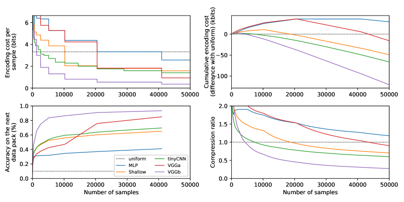
Figure 2: Prequential code results on CIFAR. Results of prequential encoding on CIFAR with 5 different models: a small Multilayer Perceptron (MLP), a shallow network, a small convolutional layer (tinyCNN), a VGG-like network without data augmentation and batch normalization (VGGa) and the same VGG-like architecture with data augmentation and batch normalization (VGGb) (see Appendix D). Performance is reported during online training, as a function of the number of samples seen so far. Top left: codelength per sample (log loss) on a pack of data $[t_{k};t_{k+1})$ given data $[1;t_{k})$. Bottom left: test accuracy on a pack of data $[t_{k};t_{k+1})$ given data $[1;t_{k})$, as a function of $t_{k}$. Top right: difference between the prequential cumulated codelength on data $[1;t_{k}]$, and the uniform encoding. Bottom right: compression ratio of the prequential code on data $[1;t_{k}]$.

Model Switching.

A weakness of prequential codes is the catch-up phenomenon (Van Erven et al., 2012). Large architectures might overfit during the first steps of the prequential encoding, when the model is trained with few data samples. Thus the encoding cost of the first packs of data might be worse than with the uniform code. Even after the encoding cost on current labels becomes lower, the cumulated codelength may need a lot of time to “catch up” on its initial lag. This can be observed in practice with neural networks: in Fig. 2, the VGGb model needs 5,000 samples on CIFAR to reach a cumulative compression ratio $<\!1$, even though the encoding cost per label becomes drops below uniform after just 1,000 samples. This is efficiently solved by switching (Van Erven et al., 2012) between models (see Appendix E). Switching further improves the practical compression bounds, even when just switching between copies of the same model with different SGD stopping times (Fig. 3, Table 2).

4 Discussion

Too Many Parameters in Deep Learning Models?

>From an information theory perspective, the goal of a model is to extract as much mutual information between the labels and inputs as possible—equivalently (Section 2.4), to compress the labels. This cannot be achieved with 2-part codes or practical network compression. With the variational code, the models do compress the data, but with a worse prediction performance: one could conclude that deep learning models that achieve the best prediction performance cannot compress the data.

Thanks to the prequential code, we have seen that deep learning models, even with a large number of parameters, compress the data well: from an information theory point of view, the number of parameters is not an obstacle to compression. This is consistent with Chaitin’s hypothesis that “comprehension is compression”, contrary to previous observations with the variational code.

Prequential Code and Generalization.

The prequential encoding shows that a model that generalizes well for every dataset size, will compress well. The efficiency of the prequential code is directly due to the generalization ability of the model at each time.

Theoretically, three of the codes (two-parts, Bayesian, and prequential based on a maximum likelihood or MAP estimator) are known to be asymptotically equivalent under strong assumptions ($d$-dimensional identifiable model, data coming from the model, suitable Bayesian prior, and technical assumptions ensuring the effective dimension of the trained model is not lower than $d$): in that case, these three methods yield a codelength $L(y_{1:n}|x_{1:n})=nH(Y|X)+\frac{d}{2}\log_{2}n+\mathcal{O}(1)$ (Grünwald, 2007). This corresponds to the BIC criterion for model selection. Hence there was no obvious reason for the prequential code to be an order of magnitude better than the others.

However, deep learning models do not usually satisfy any of these hypotheses. Moreover, our prequential codes are not based on the maximum likelihood estimator at each step, but on standard deep learning methods (so training is regularized at least by dropout and early stopping).

Inefficiency of Variational Models for Deep Networks.

The objective of variational methods is equivalent to minimizing a description length. Thus, on our image classification tasks, variational methods do not have good results even for their own objective, compared to prequential codes. This makes their relatively poor results at test time less surprising.

Understanding this observed inefficiency of variational methods is an open problem. As stated in (3.4), the variational codelength is an upper bound for the Bayesian codelength. More precisely,

$$L_{\beta}^{\mathrm{var}}(y_{1:n}|x_{1:n})=L^{\mathrm{Bayes}}(y_{1:n}|x_{1:n})+\operatorname{{\mathrm{KL}}}\left(p_{\mathrm{Bayes}}(\theta|x_{1:n},y_{1:n})\|\beta\right)$$ (4.1)

with notation as above, and with $p_{\mathrm{Bayes}}(\theta|x_{1:n},y_{1:n})$ the Bayesian posterior on $\theta$ given the data. Empirically, on MNIST and CIFAR, we observe that $L^{\mathrm{preq}}(y_{1:n}|x_{1:n})\ll L_{\beta}^{\mathrm{var}}(y_{1:n}|x_{1:n}).$

Several phenomena could contribute to this gap. First, the optimization of the parameters $\phi$ of the approximate Bayesian posterior might be imperfect. Second, even the optimal distribution $\beta^{*}$ in the variational class might not approximate the posterior $p_{\mathrm{Bayes}}(\theta|x_{1:n},y_{1:n})$ well, leading to a large $\operatorname{{\mathrm{KL}}}$ term in (4.1); this would be a problem with the choice of variational posterior class $\beta$. On the other hand we do not expect the choice of Bayesian prior to be a key factor: we tested Gaussian priors with various variances as well as a conjugate Gaussian prior, with similar results. Moreover, Gaussian initializations and L2 weight decay (acting like a Gaussian prior) are common in deep learning. Finally, the (untractable) Bayesian codelength based on the exact posterior might itself be larger than the prequential codelength. This would be a problem of underfitting with parametric Bayesian inference, perhaps related to the catch-up phenomenon or to the known conservatism of Bayesian model selection (end of Section 3.3).

5 Conclusion

Deep learning models can represent the data together with the model in fewer bits than a naive encoding, despite their many parameters. However, we were surprised to observe that variational inference, though explicitly designed to minimize such codelengths, provides very poor such values compared to a simple incremental coding scheme. Understanding this limitation of variational inference is a topic for future research.

Appendix A Fake labels are not compressible

In the introduction, we stated that fake labels could not be compressed. This means that the optimal codelength for this labels is almost the uniform one. This can be formalized as follows. We define a code for $y_{1:n}$ as any program (in a reference Turing machine) that outputs $y_{1:n}$, and denote $L(y_{1:n})$ the length of this program, or $L(y_{1:n}|x_{1:n})$ for programs that may use $x_{1:n}$ as their input.

Proposition 2.

Assume that $x_{1},...,x_{n}$ are inputs, and that $Y_{1},...,Y_{n}$ are iid random labels uniformly sampled in $\{1,...,K\}$. Then for any $\delta\in\mathbb{N}^{*}$, with probability $1-2^{-\delta}$ the values $Y_{1},\ldots,Y_{n}$ satisfy that for any possible coding procedure $L$ (even depending on the values of $x_{1:n}$), the codelength of $Y_{1:n}$ is at least

$$L(Y_{1:n}|x_{1:n}) \geq nH(Y)-\delta-1$$ (A.1)

$$=n\log_{2}K-\delta-1.$$ (A.2)

We insist that this does not require any assumptions on the coding procedure used, so this result holds for all possible models. Moreover, this is really a property of the sampled values $Y_{1},\ldots Y_{n}$: most values of $Y_{1:n}$ can just not be compressed by any algorithm.

Proof.

This proposition is a standard counting argument, or an immediate consequence of Theorem 2.2.1 in (Li and Vitányi, 2008). Let $\mathcal{A}=\{1,...,K\}^{n}$ be the set of all possible outcomes for the sequence of random labels. We have $|\mathcal{A}|=K^{n}$. Let $\delta$ be an integer, $\delta\in\mathbb{N}^{*}$, we want to know how many elements in $\mathcal{A}$ can be encoded in less than $\log_{2}|\mathcal{A}|-\delta$ bits. We consider, on a given Turing machine, the number of programs of length less than $\lfloor\log_{2}|\mathcal{A}|-\delta\rfloor$. This number is less than :

$$\sum_{i=0}^{\lfloor\log_{2}|\mathcal{A}|\rfloor-\delta-1}2^{i} =2^{\lfloor\log_{2}|\mathcal{A}|\rfloor-\delta}-1$$ (A.3)

$$\leq 2^{-\delta}|\mathcal{A}|-1$$ (A.4)

Therefore, the number of elements in $\mathcal{A}$ which can be described in less than $\log_{2}|\mathcal{A}|-\delta$ bits is less than $2^{-\delta}|\mathcal{A}|-1$. We can deduce from this that the number of elements in $\mathcal{A}$ which cannot be described by any program in less than $2^{-\delta}|\mathcal{A}|-1$ bits is at least $|\mathcal{A}|(1-2^{-\delta})$. Equivalently, there are at least $|\mathcal{A}|(1-2^{-\delta})$ elements $(y_{1},...,y_{n})$ in $|\mathcal{A}|$ such that for any coding scheme, $L(y_{1:n}|x_{1:n})\geq n\log_{2}K-\delta-1$. Since the random labels $Y_{1},...,Y_{n}$ are uniformly distributed, the result follows. ∎

Appendix B Technical details on compression bounds with random affine subspaces

We describe in Algorithm 1 the detailed procedure which allows to compute compression bounds with the random affine subspace method (Li et al., 2018). To compute the numerical results in Table 1, we took the intrinsic dimension computed in the original paper, and considered that the precision of the parameter was 32 bits, following the authors’ suggestion. Then, the description length of the model itself is $32\times$ the intrinsic dimension. This does not take into account the description length of the labels given the model, which is non-negligible (to take this quantity into account, we would need to know the loss on the training set of the model, which was not specified in the original paper). Thus we only get a lower bound.

Algorithm 1 Encoding with random affine subspaces

  Alice transmits a parametric model $(p_{\theta})_{\theta\in\Theta}$.

  Alice transmits the random seed $\omega$ (if using stochastic optimization), and a dimension $k$.

  Alice and Bob both sample a random affine subspace $\tilde{\Theta}\subset\Theta$, with the seed $\omega$. This means that they sample $\theta_{0}$ and a matrix $W$ of dimension $k\times d$ where $d$ is the dimension of $\Theta$. It defines a new parametric model $\tilde{p}_{\phi}=p_{\theta_{0}+W\cdot\phi}$

  Alice optimizes the parameter $\phi^{*}$ with a gradient descent algoritm in order to minimize $-\log_{2}\tilde{p}_{\phi}(y_{1:n}|x_{1:n})$.

  Alice sends $\phi^{*}$ with a precision $\varepsilon$ to Bob. It costs $k\times\log_{2}\varepsilon$.

  Alice sends the labels $y_{1:n}$ with the models $\tilde{p}_{\phi^{*}}$. It costs $-\log_{2}\tilde{p}_{\phi^{*}}(y_{1:n}|x_{1:n})$

For MNIST, the model with the smaller intrinsic dimension is the LeNet, which has an intrinsic dimension of 290 for an accuracy of $90\%$ (the threshold at which (Li et al., 2018) stop by definition, hence the performance in Table 1). This leads to a description length for the model of $9280$ bits, which corresponds to a $0.05$ compression ratio, without taking into account the description length of the labels given the model.

For CIFAR, again with the LeNet architecture, the intrinsic dimension is 2,900. This leads to a description length for the model of $92800$ bits, which corresponds to a $0.05$ compression ratio, without taking into account the description length of the labels given the model.

These bounds could be improved by optimizing the precision $\varepsilon$. Indeed, reducing the precision makes the model less accurate and increases the encoding cost of the labels with the model, but it decreases the encoding cost of the parameters. Therefore, we could find an optimal precision $\varepsilon^{*}$ to improve the compression bound. This would be a topic for future work.

Appendix C Technical Details on Variational Learning for Section 3.3

Variational learning was performed using the library Pyvarinf (Tallec and Blier, 2018).

We used a prior $\alpha=\mathcal{N}(0,\sigma_{0}^{2}I_{d})$ with $\sigma_{0}=0.05$, chosen to optimize the compression bounds.

The chosen class of posterior was the class of multivariate gaussian distributions with diagonal covariance matrix $\{\mathcal{N}(\mu,\Sigma)\;,\;\mu\in\mathbb{R}^{d}\;\Sigma\;\mathrm{diagonal}\}$. It was parametrized by $(\beta_{\mu,\rho})_{(\mu,\rho)\in\mathbb{R}^{d}\times\mathbb{R}^{d}}$, with $\sigma\in\mathbb{R}^{d}$ defined as $\sigma_{i}=\log(1+\exp({\rho_{i}}))$, and the covariance matrix $\Sigma$ as the diagonal matrix with diagonal values $\sigma_{1}^{2},...,\sigma_{d}^{2}$.

We optimize the bound (3.2) as a function of ($\mu,\rho$) with a gradient descent method, and estimate its values and gradient with a Monte-Carlo method. Since the prior and posteriors are gaussian, we have an explicit formula for the first part of the variational loss $\operatorname{{\mathrm{KL}}}(\beta_{\mu,\rho}\|\alpha)$ (Hinton and Van Camp, 1993). Therefore, we can easily compute its values and gradients. For the second part

$$(\mu,\rho)\rightarrow\mathbb{E}_{\theta\sim\beta_{\mu,\rho}}\bigg{[}\sum_{i=1}^{n}-\log_{2}p_{\theta}(y_{i}|x_{i})\bigg{]},$$ (C.1)

we can use the following proposition (Graves, 2011). For any function $f\colon\Theta\rightarrow\mathbb{R}$, we have

$$\frac{\partial}{\partial\mu_{i}}\mathbb{E}_{\theta\sim\beta_{\mu,\rho}}[f(\theta)] =\mathbb{E}_{\theta\sim\beta_{\mu,\rho}}\Big{[}\frac{\partial f}{\partial\theta_{i}}(\theta)\Big{]}$$ (C.2)

$$\frac{\partial}{\partial\rho_{i}}\mathbb{E}_{\theta\sim\beta_{\mu,\rho}}[f(\theta)] =\frac{\partial\sigma_{i}}{\partial\rho_{i}}\cdot\mathbb{E}_{\theta\sim\beta_{\mu,\rho}}\Big{[}\frac{\partial f}{\partial\theta_{i}}\cdot\frac{\theta_{i}-\mu_{i}}{\sigma_{i}}\Big{]}$$ (C.3)

Therefore, we can estimate the values and gradients of (3.2) with a Monte-Carlo algorithm:

$$\frac{\partial}{\partial\mu_{i}}\mathbb{E}_{\theta\sim\beta_{\mu,\rho}}[f(\theta)] \approx\sum_{s=1}^{S}\frac{\partial f}{\partial\theta_{i}}(\theta^{s})$$ (C.4)

$$\frac{\partial}{\partial\rho_{i}}\mathbb{E}_{\theta\sim\beta_{\mu,\rho}}[f(\theta)] \approx\frac{\partial\sigma_{i}}{\partial\rho_{i}}\cdot\sum_{s=1}^{S}\frac{\partial f}{\partial\theta_{i}}(\theta^{s})\cdot\frac{\theta^{s}_{i}-\mu_{i}}{\sigma_{i}}$$ (C.5)

where $\theta^{1},...,\theta^{S}$ are sampled from $\beta_{\mu,\rho}$. In practice, we used $S=1$ both for the computations of the variational loss and its gradients.

We used both convolutional and fully connected architectures, but in our experiments fully connected models were better for compression. For CIFAR and MNIST, we used fully connected networks with two hidden layers of width 256, trained with SGD, with a $0.005$ learning rate and mini-batchs of size 128.

For CIFAR and MNIST, we used a LeNet-like network with 2 convolutional layers with 6 and 16 filters, both with kernels of size 5 and 3 fully connected layers. Each convolutional is followed by a ReLU activation and a max-pooling layer. The code will be publicly available. The first and the second fully connected layers are of dimension 120 and 84 and are followed by ReLU activations. The last one is followed by a softmax activation layer. The code for all models will be publicly available.

During the test phase, we sampled parameters $\hat{\theta}$ from the learned distribution $\beta$, and used the model $p_{\hat{\theta}}$ for prediction. This explains why our test accuracy on MNIST is lower than other numerical results (Blundell et al., 2015), since they use for prediction the averaged model with parameters $\hat{\theta}=\mathbb{E}_{\theta\sim\beta_{m,r}}[\theta]=\mu$. But our goal was not to get the best prediction score, but to evaluate the model which was used for compression on the test set.

Appendix D Technical details on prequential learning

Prequential Learning on MNIST.

On MNIST, we used three different models:

1. The uniform probability over the labels.

2. A fully connected network or Multilayer Perceptron (MLP) with two hidden layers of dimension 256.

3. A VGG-like convolutional network with 8 convolutional layers with 32, 32, 64, 64, 128, 128, 256 and 256 filters respectively and max pooling operators every two convolutional layers, followed by two fully connected layers of size 256.

For the two neural networks we used Dropout with probability $0.5$ between the fully connected layers, and optimized the network with the Adam algorithm with learning rate $0.001$.

The successive timestep for the prequential learning $t_{1},t_{2},...,t_{s}$ are 8, 16, 32, 64, 128, 256, 512, 1024, 2048, 4096, 8192, 16384 and 32768.

For the prequential code results in Table 1, we selected the best model, which was the VGG-like network.

Prequential Learning on CIFAR.

On CIFAR, we used five different models:

1. The uniform probability over the labels.

2. A fully connected network or Multilayer Perceptron (MLP) with two hidden layers of dimension 512.

3. A shallow network, with one hidden layer and width 5000.

4. A convolutional network (tinyCNN) with four convolutional layers with 32 filters, and a maxpooling operator after every two convolutional layers. Then, two fully connected layers of dimension 256. We used Dropout with probability $0.5$ between the fully connected layers.

5. A VGG-like network with 13 convolutional layers from (Zagoruyko, 2015). We trained this architecture with two learning procedures. The first one (VGGa) without batch-normalization and data augmentation, and the second one (VGGb) with both of them, as introduced in (Zagoruyko, 2015). In both of them, we used dropout regularization with parameter 0.5.

We optimized the network with the Adam algorithm with learning rate 0.001.

For prequential learning, the timesteps $t_{1},t_{2},...,t_{s}$ were: 10, 20, 40, 80, 160, 320, 640, 1280, 2560, 5120, 10240, 20480, 40960. The training results can be seen in Figure 2.

For the prequential code, all the results are in Figure 2. For the results in Table 1, we selected the best model for the prequential code, which was VGGb.

Algorithm 2 Prequential encoding

  Input: data $x_{1:n},y_{1:n}$, timesteps $1=t_{0}<t_{1}<...<t_{S}=n$

  Alice transmits the random seed $\omega$ (if using stochastic optimization).

  Alice encodes $y_{1:t_{1}}$ with the uniform code. This costs $t_{1}\log_{2}K$ bits. Bob decodes $y_{1:t_{1}}$.

  for $s=1$ to $S-1$ do

     Alice and Bob both compute $\hat{\theta}_{s}=\hat{\theta}(x_{1:t_{s}},y_{1:t_{s}},\omega)$.

     Alice encodes $y_{t_{s}+1:t_{s+1}}$ with model $p_{\hat{\theta}_{s}}$. This costs $-\log_{2}p_{\hat{\theta}_{s}}(y_{t_{s}+1:t_{s+1}}|x_{t_{s}+1:t_{s+1}})$ bits

     Bob decodes $y_{t_{s}+1:t_{s+1}}$

  end for

Appendix E Switching between models against the catch-up phenomenon

Table 2: Compression bounds by switching between models. Compression bounds given by different codes on two datasets, MNIST and CIFAR10. The Codelength is the number of bits necessary to send the labels to someone who already has the inputs. This codelength includes the description length of the model. The compression ratio for a given code is the ratio between its codelength and the codelength of the uniform code. The test accuracy of a model is the accuracy of its predictions on the test set. For variational and prequential codes, we selected the model and hyperparameters providing the best compression bound.

Code	mnist			cifar10
	Codelength	Comp.	Test	Codelength	Comp.	Test
	($\operatorname{kbits}$)	Ratio	Acc	($\operatorname{kbits}$)	Ratio	Acc
Uniform	199	1.	10%	166	1.	10%
Variational	24.1	0.12	95.5%	89.0	0.54	61,6%
Prequential	4.10	0.02	99.5%	45.3	0.27	93.3%
Switch	4.05	0.02	99.5%	34.6	0.21	93.3%
Self-Switch	4.05	0.02	99.5%	34.9	0.21	93.3%

E.1 Switching between model classes

The solution introduced by (Van Erven et al., 2012) against the catch-up phenomenon described in Section 3.4, is to switch between models, to always encode a data block with the best model at that point. That way, the encoding adapts itself to the number of data samples seen. The switching pattern itself has to be encoded.

Assume that Alice and Bob have agreed on a set of prediction strategies $\mathcal{M}=\{p^{k},k\in\mathcal{I}\}$. We define the set of switch sequences, $\mathbb{S}=\{((t_{1},k_{1}),...,(t_{L},k_{L})),1=t_{1}<t_{2}<...<t_{L}\;,\;k\in\mathcal{I}\}$.

Let $s=((t_{1},k_{1}),...,(t_{L},k_{L}))$ be a switch sequence. The associated prediction strategy $p_{s}(y_{1:n}|x_{1:n})$ uses model $p^{k_{i}}$ on the time interval $[t_{i};t_{i+1})$, namely

$$p_{s}(y_{1:i+1}|x_{1:i+1},y_{1:i})=p^{K_{i}}(y_{i+1}|x_{1:i+1},y_{1:i})$$ (E.1)

where $K_{i}$ is such that $K_{i}=k_{l}$ for $t_{l}\leq i<t_{l+1}$. Fix a prior distribution $\pi$ over switching sequences (see (Van Erven et al., 2012) for typical examples).

Definition 4 (Switch code).

Assume that Alice and Bob have agreed on a set of prediction strategies $\mathcal{M}$ and a prior $\pi$ over $\mathbb{S}$. The switch code first encodes a switch sequence $s$ strategy, then uses the prequential code with this strategy:

$$L_{s}^{\mathrm{sw}}(y_{1:n},x_{1:n})=L_{\pi}(s)+L^{\mathrm{preq}}_{p_{s}}(y_{1:n},x_{1:n})=-\log_{2}\pi(s)-\sum_{i=1}^{n}\log_{2}p^{K_{i}}(y_{i}|x_{1:i},y_{1:i-1})$$ (E.2)

where $K_{i}$ is the model used by switch sequence $s$ at time $i$.

We then choose the switching strategy $s^{*}$ wich minimizes $L_{s}^{\mathrm{sw}}(y_{1:n},x_{1:n})$. We tested switching between the uniform model, a small convolutional network (tinyCNN), and a VGG-like network with two training methods (VGGa, VGGb) (Appendix D). On MNIST, switching between models does not make much difference. On CIFAR10, switching by taking the best model on each interval $[t_{k};t_{k+1})$ saves more than $11\operatorname{kbits}$, reaching a codelength of $34.6\operatorname{kbits}$, and a compression ratio of $0.21$. The cost $L_{\pi}(s)$ of encoding the switch $s$ is negligible (see Table 2).

E.2 Self-Switch: Switching between variants of a model or hyperparameters

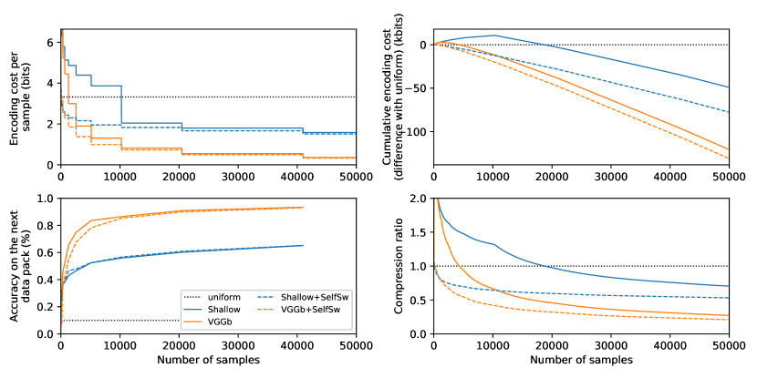
Figure 3: Compression with the self-switch method: Results of the self-switch code on CIFAR with 2 different models: the shallow network, and the VGG-like network trained with data augmentation and batch normalization (VGGb). Performance is reported during online training, as a function of the number of samples seen so far. Top: test accuracy on a pack of data $[t_{k};t_{k+1})$ given data $[1;t_{k})$, as a function of $t_{k}$. Second: codelength per sample (log loss) on a pack of data $[t_{k};t_{k+1})$ given data $[1;t_{k})$. Third: difference between the prequential cumulated codelength on data $[1;t_{k}]$, and the uniform encoding. Bottom: compression ratio of the prequential code on data $[1;t_{k}]$. The catch-up phenomenon is clearly visible for both models: even if models with and without the self-switch have similar performances after a training on the entire dataset, the standard model has lower performances than the uniform model (for the 1280 first labels for the VGGb network, and for the 10,000 first labels for the shallow network), and the code length for these first labels is large. The self-switch method solves this problem.

With standard switch, it may be cumbersome to work with different models in parallel. Instead, for models learned by gradient descent, we may use the same architecture but with different parameter values corresponding obtained at different gradient descent stopping times. This is a form of regularization via early stopping.

Let $(p_{\theta})_{\theta\in\Theta}$ be a model class. Let $\hat{\theta}_{j}(x_{1:k},y_{1:k})$ be the parameter obtained by some optimization procedure after $j$ epochs of training on data $[1;k]$. For instance, $j=0$ would correspond to using an untrained model (usually close to the uniform model).

We call self-switch code the switch code obtained by switching among the family of models with different gradient descent stopping times $j$ (based on the same parametric family $(p_{\theta})_{\theta\in\Theta}$). In practice, this means that at each step of the prequential encoding, after having seen data $[1;t_{k})$, we train the model on those data and record, at each epoch $j$, the loss obtained on data $[t_{k};t_{k+1})$. We then switch optimally between those. We incur the small additional cost of encoding the best number of epochs to be used (which was limited to $10$) at each step.

The catch-up phenomenon and the beneficial effect of the self-switch code can be seen in Figure 3.

The self-switch code achieves similar compression bounds to the switch code, while storing only one network. On MNIST, there is no observable difference. On CIFAR, self-switch is only 300 bits (0.006 bit/label) worse than full $4$-architecture switch.

References

- Achille and Soatto (2017) A. Achille and S. Soatto. On the Emergence of Invariance and Disentangling in Deep Representations. arXiv preprint arXiv:1706.01350, jun 2017. URL http://arxiv.org/abs/1706.01350.
- Arora et al. (2018) S. Arora, R. Ge, B. Neyshabur, and Y. Zhang. Stronger generalization bounds for deep nets via a compression approach. arXiv preprint arXiv:1802.05296, 2018.
- Ba and Caruana (2014) L. J. Ba and R. Caruana. Do Deep Nets Really Need to be Deep? In Advances in Neural Information Processing Systems, pages 2654–2662, 2014.
- Barron and Yang (1999) A. Barron and Y. Yang. Information-theoretic determination of minimax rates of convergence. The Annals of Statistics, 27(5):1564–1599, 1999.
- Blum and Langford (2003) A. Blum and J. Langford. PAC-MDL Bounds. In B. Schölkopf and M. K. Warmuth, editors, Learning Theory and Kernel Machines, pages 344–357, Berlin, Heidelberg, 2003. Springer Berlin Heidelberg. ISBN 978-3-540-45167-9.
- Blundell et al. (2015) C. Blundell, J. Cornebise, K. Kavukcuoglu, and D. Wierstra. Weight Uncertainty in Neural Networks. In International Conference on Machine Learning, pages 1613–1622, 2015.
- Chaitin (2007) G. J. Chaitin. On the intelligibility of the universe and the notions of simplicity, complexity and irreducibility. In Thinking about Godel and Turing: Essays on Complexity, 1970-2007. World scientific, 2007.
- Dawid (1984) A. P. Dawid. Present Position and Potential Developments: Some Personal Views: Statistical Theory: The Prequential Approach. Journal of the Royal Statistical Society. Series A (General), 147(2):278, 1984.
- Dziugaite and Roy (2017) G. K. Dziugaite and D. M. Roy. Computing Nonvacuous Generalization Bounds for Deep (Stochastic) Neural Networks with Many More Parameters than Training Data. In Proceedings of the Thirty-Third Conference on Uncertainty in Artificial Intelligence, Sydney, 2017.
- Foster and George (1994) D. P. Foster and E. I. George. The Risk Inflation Criterion for Multiple Regression. The Annals of Statistics, 22(4):1947–1975, dec 1994.
- Gao and Jojic (2016) T. Gao and V. Jojic. Degrees of Freedom in Deep Neural Networks. arXiv preprint arXiv:1603.09260, mar 2016.
- Graves (2011) A. Graves. Practical Variational Inference for Neural Networks. In Neural Information Processing Systems, 2011.
- Grünwald (2007) P. D. Grünwald. The Minimum Description Length principle. MIT press, 2007.
- Han et al. (2015a) S. Han, H. Mao, and W. J. Dally. Deep Compression: Compressing Deep Neural Networks with Pruning, Trained Quantization and Huffman Coding. arXiv preprint arXiv:1510.00149, 2015a.
- Han et al. (2015b) S. Han, J. Pool, J. Tran, and W. J. Dally. Learning both Weights and Connections for Efficient Neural Networks. In Advances in Neural Information Processing Systems, 2015b.
- Hinton and Van Camp (1993) G. E. Hinton and D. Van Camp. Keeping Neural Networks Simple by Minimizing the Description Length of the Weights. In Proceedings of the sixth annual conference on Computational learning theory. ACM, 1993.
- Honkela and Valpola (2004) A. Honkela and H. Valpola. Variational Learning and Bits-Back Coding: An Information-Theoretic View to Bayesian Learning. IEEE transactions on Neural Networks, 15(4), 2004.
- Hutter (2007) M. Hutter. On Universal Prediction and Bayesian Confirmation. Theoretical Computer Science, 384(1), sep 2007.
- Ioffe and Szegedy (2015) S. Ioffe and C. Szegedy. Batch Normalization: Accelerating Deep Network Training by Reducing Internal Covariate Shift. In International Conference on Machine Learning, pages 448–456, 2015.
- Kingma and Welling (2013) D. P. Kingma and M. Welling. Auto-Encoding Variational Bayes. arXiv preprint arXiv:1312.6114, 2013.
- Krizhevsky (2009) A. Krizhevsky. Learning Multiple Layers of Features from Tiny Images. 2009.
- Kucukelbir et al. (2017) A. Kucukelbir, D. Tran, R. Ranganath, A. Gelman, and D. M. Blei. Automatic Differentiation Variational Inference. Journal of Machine Learning Research, 18:1–45, 2017.
- LeCun et al. (1998) Y. LeCun, L. Bottou, Y. Bengio, and P. Haffner. Gradient-Based Learning Applied to Document Recognition. Proceedings of the IEEE, 86(11), 1998.
- LeCun et al. (2015) Y. LeCun, Y. Bengio, and G. Hinton. Deep learning. Nature, 521(7553):436–444, 2015.
- Li et al. (2018) C. Li, H. Farkhoor, R. Liu, and J. Yosinski. Measuring the Intrinsic Dimension of Objective Landscapes. arXiv preprint arXiv:1804.08838, apr 2018.
- Li and Vitányi (2008) M. Li and P. Vitányi. An introduction to Kolmogorov complexity. Springer, 2008.
- Louizos et al. (2017) C. Louizos, K. Ullrich, and M. Welling. Bayesian compression for deep learning. In Advances in Neural Information Processing Systems, pages 3290–3300, 2017.
- Mackay (2003) D. J. C. Mackay. Information Theory, Inference, and Learning Algorithms. Cambridge University Press, cambridge edition, 2003.
- Ollivier (2014) Y. Ollivier. Auto-encoders: reconstruction versus compression. arXiv preprint arXiv:1403.7752, mar 2014. URL http://arxiv.org/abs/1403.7752.
- Rissanen (2007) J. Rissanen. Information and complexity in statistical modeling. Springer Science & Business Media, 2007.
- Rissanen et al. (1992) J. Rissanen, T. Speed, and B. Yu. Density estimation by stochastic complexity. IEEE Transactions on Information Theory, 38(2):315–323, 1992.
- Romero et al. (2015) A. Romero, N. Ballas, S. E. Kahou, A. Chassang, C. Gatta, and Y. Bengio. Fitnets: Hints for thin deep nets. In Proceedings of the International Conference on Learning Representations, 2015.
- Schmidhuber (1997) J. Schmidhuber. Discovering Neural Nets with Low Kolmogorov Complexity and High Generalization Capability. Neural Networks, 10(5):857–873, jul 1997.
- See et al. (2016) A. See, M.-T. Luong, and C. D. Manning. Compression of Neural Machine Translation Models via Pruning. arXiv preprint arXiv:1606.09274, 2016.
- Shannon (1948) C. Shannon. A mathematical theory of communication. The Bell System Technical Journal, 27, 1948.
- Shwartz-Ziv and Tishby (2017) R. Shwartz-Ziv and N. Tishby. Opening the Black Box of Deep Neural Networks via Information. arXiv preprint arXiv:1703.00810, 2017.
- Simonyan and Zisserman (2014) K. Simonyan and A. Zisserman. Very Deep Convolutional Networks for Large-Scale Image Recognition. arXiv preprint arXiv:1409.1556, sep 2014.
- Solomonoff (1964) R. Solomonoff. A formal theory of inductive inference. Information and control, 1964.
- Tallec and Blier (2018) C. Tallec and L. Blier. Pyvarinf : Variational Inference for PyTorch, 2018. URL https://github.com/ctallec/pyvarinf.
- Tishby and Zaslavsky (2015) N. Tishby and N. Zaslavsky. Deep Learning and the Information Bottleneck Principle. In Information Theory Workshop, pages 1–5. IEEE, 2015.
- Ullrich et al. (2017) K. Ullrich, E. Meeds, and M. Welling. Soft Weight-Sharing for Neural Network Compression. arXiv preprint arXiv:1702.04008, 2017.
- Van Erven et al. (2012) T. Van Erven, P. Grünwald, and S. De Rooij. Catching Up Faster by Switching Sooner: A predictive approach to adaptive estimation with an application to the AIC-BIC Dilemma. Journal of the Royal Statistical Society: Series B (Statistical Methodology), 74(3):361–417, 2012.
- Xu et al. (2017) T.-B. Xu, P. Yang, X.-Y. Zhang, and C.-L. Liu. Margin-Aware Binarized Weight Networks for Image Classification. In International Conference on Image and Graphics, pages 590–601. Springer, Cham, sep 2017.
- Zagoruyko (2015) S. Zagoruyko. 92.45% on CIFAR-10 in Torch, 2015. URL http://torch.ch/blog/2015/07/30/cifar.html.
- Zhang et al. (2017) C. Zhang, S. Bengio, M. Hardt, B. Recht, and O. Vinyals. Understanding deep learning requires rethinking generalization. In Proceedings of the International Conference on Learning Representations, 2017.