Hairy black hole solutions in $U(1)$ gauge-invariant scalar-vector-tensor theories

Abstract

In $U(1)$ gauge-invariant scalar-vector-tensor theories with second-order equations of motion, we study the properties of black holes (BH) on a static and spherically symmetric background. In shift-symmetric theories invariant under the shift of scalar $\phi\to\phi+c$, we show the existence of new hairy BH solutions where a cubic-order scalar-vector interaction gives rise to a scalar hair manifesting itself around the event horizon. In the presence of a quartic-order interaction besides the cubic coupling, there are also regular BH solutions endowed with scalar and vector hairs.

I Introduction

On the contrary to the geometrical interpretation of gravitational physics, the description in terms of field theory is unambiguous. It relies on the uniqueness of interactions of a massless spin-2 particle. The constructed Lagrangian inevitably leads to General Relativity (GR) with two propagating tensor degrees of freedom and with second-order equations of motion.

The extension from GR to modified gravity theories generally introduces new degrees of freedom besides two tensor polarizations review . Under the assumptions of pseudo-Riemannian space-time, Lorentz symmetry, and locality, one can construct consistent tensor-tensor, vector-tensor and scalar-tensor theories with additional tensor, vector or scalar fields in the gravity sector. Modified gravity theories based on an additional scalar field $\phi$ have been most extensively studied by reflecting their simplicity. Fixing the ingredients of gravitational theory to be one spin-0 field besides two tensor polarizations, it is possible to construct most general scalar-tensor theories with second-order equations of motion, known as Horndeski theories Horndeski:1974wa ; Horndeskire . The resulting action contains derivative and non-minimal couplings to gravity without inducing Ostragradski instabilities.

Instead of a scalar field, one can introduce an additional spin-1 field into the gravity sector with a richer phenomenology due to the existence of intrinsic vector modes. Analogous to scalar-tensor Horndeski theories, it is possible to construct most general vector-tensor theories with second-order equations of motion. Upon imposing the $U(1)$ gauge invariance of the vector field $A_{\mu}$, Horndeski obtained a single nonminimal coupling of the vector field to the double dual Riemann tensor Horndeski:1976gi without vector derivative self-interactions. If one abandons the gauge invariance like the case of a massive vector filed, there are derivative and nonminimal couplings to gravity giving rise to generalized Proca theories Heisenberg:2014rta . Even if the longitudinal mode of the vector field behaves as the Horndeski scalar field, there are two important purely intrinsic vector interactions with no scalar counterpart Heisenberg:2014rta ; Jimenez:2016isa (see also Refs. VectorTensorTheories ). The relevance of these vector-tensor theories for cosmology VTcosmoearly ; VTcosmology and compact objects screening ; VTastrophys1 ; VTastrophys2 ; VTastrophys3 has been already extensively studied in the literature.

One can unify these two important classes of Horndeski and generalized Proca theories into the framework of scalar-vector-tensor (SVT) theories. In Ref. Heisenberg18 , the construction of SVT theories with second-order equations of motion was performed for both the $U(1)$ gauge-invariant and the non gauge-invariant cases. The new degrees of freedom arising in SVT theories may be relevant to the physics of black holes, inflation, dark energy, dark matter and the generation of magnetic fields. In light of the detection of gravitational waves from BH and neutron star mergers GW1 ; GW2 , it is of interest to study whether or not some “hairs” associated with the new degrees of freedom arise on a strong gravitational background.

In this letter, we study BH solutions in $U(1)$ gauge-invariant SVT theories on a static and spherically symmetric background. We show that the existence of cubic-order scalar-vector interactions allows the possibility for realizing a nontrivial scalar-field configuration. In shift-symmetric theories where the Lagrangian is invariant under the shift $\phi\to\phi+c$, there exist new hairy BH solutions with scalar hair supported by the scalar-vector interaction. We derive iterative solutions both in the vicinity of the horizon and at spatial infinity for the theories containing cubic and quartic interactions. We note that some BH solutions have been discussed in Ref. Cha for the quartic interaction, but we will show that the cubic interaction is crucially important for the existence of BHs with scalar hair. We will also numerically confirm the regularity of solutions outside the horizon exterior.

This letter is organized as follows. In Sec. II, we revisit $U(1)$ gauge-invariant SVT theories and present the background equations of motion on the static and spherically symmetric spacetime. In Sec. III, we show the existence of regular BH solutions with scalar hair for a cubic-order coupling. In Sec. IV, we extend the analysis to the case in which quartic-order interactions are present besides the cubic coupling. We conclude in Sec. V.

II Gauge-invariant SVT theories and equations of motion

In Ref. Heisenberg18 , the SVT theories were constructed for both $U(1)$ gauge-invariant and broken gauge-invariant cases. In this letter, we will focus on the gauge-invariant case. The most general gauge-invariant action of SVT theories with second-order equations of motion is expressed in the form

$$\mathcal{S}=\int d^{4}x\sqrt{-g}\left(\sum_{i=3}^{5}\mathcal{L}^{i}_{\rm ST}+\sum_{i=2}^{4}\mathcal{L}^{i}_{\rm SVT}\right)\,,$$ (1)

where $g$ is a determinant of the metric tensor $g_{\mu\nu}$, and $\mathcal{L}^{3}_{\rm ST},\mathcal{L}^{4}_{\rm ST},\mathcal{L}^{5}_{\rm ST}$ are the cubic, quartic, and quintic Lagrangians in pure scalar Horndeski theories with a scalar field $\phi$ Horndeski:1974wa ; Horndeskire . The other Lagrangians $\mathcal{L}^{2}_{\rm SVT},\mathcal{L}^{3}_{\rm SVT},\mathcal{L}^{4}_{\rm SVT}$ correspond to the genuine scalar-vector-tensor interactions, whose explicit forms are given, respectively, by

$$\mathcal{L}^{2}_{\rm SVT} = f_{2}(\phi,X,F,\tilde{F},Y)\,,$$ (2)

$$\mathcal{L}^{3}_{\rm SVT} = \mathcal{M}_{3}^{\mu\nu}\nabla_{\mu}\nabla_{\nu}\phi\,,$$ (3)

$$\mathcal{L}^{4}_{\rm SVT} = \mathcal{M}_{4}^{\mu\nu\alpha\beta}\nabla_{\mu}\nabla_{\alpha}\phi\nabla_{\nu}\nabla_{\beta}\phi+f_{4}(\phi,X)L^{\mu\nu\alpha\beta}F_{\mu\nu}F_{\alpha\beta}\,,$$ (4)

where

$$X=-\frac{1}{2}\nabla_{\mu}\phi\nabla^{\mu}\phi\,,\qquad F=-\frac{1}{4}F_{\mu\nu}F^{\mu\nu}\,,\qquad\tilde{F}=-\frac{1}{4}F_{\mu\nu}\tilde{F}^{\mu\nu}\,,\qquad Y=\nabla_{\mu}\phi\nabla_{\nu}\phi F^{\mu\alpha}{F^{\nu}}_{\alpha}\,,$$ (5)

with the gauge-invariant field strength $F_{\mu\nu}=\nabla_{\mu}A_{\nu}-\nabla_{\nu}A_{\mu}$ and the dual strength tensor $\tilde{F}^{\mu\nu}=\mathcal{E}^{\mu\nu\alpha\beta}F_{\alpha\beta}/2$. Here, $\mathcal{E}^{\mu\nu\alpha\beta}$ is the anti-symmetric Levi-Civita tensor satisfying the normalization $\mathcal{E}^{\mu\nu\alpha\beta}\mathcal{E}_{\mu\nu\alpha\beta}=-4!$. The rank-2 tensor $\mathcal{M}_{3}^{\mu\nu}$ in the Lagrangian $\mathcal{L}^{3}_{\rm SVT}$ is of the form

$$\mathcal{M}^{\mu\nu}_{3}=\left[f_{3}(\phi,X)g_{\rho\sigma}+\tilde{f}_{3}(\phi,X)\nabla_{\rho}\phi\nabla_{\sigma}\phi\right]\tilde{F}^{\mu\rho}\tilde{F}^{\nu\sigma}\,,$$ (6)

where $f_{3}$ and $\tilde{f}_{3}$ are functions of $\phi$ and $X$. Similarly, the rank-4 tensor $\mathcal{M}_{4}^{\mu\nu\alpha\beta}$ is constrained to be

$$\mathcal{M}^{\mu\nu\alpha\beta}_{4}=\left[\frac{1}{2}f_{4,X}(\phi,X)+\tilde{f}_{4}(\phi)\right]\tilde{F}^{\mu\nu}\tilde{F}^{\alpha\beta}\,,$$ (7)

where $f_{4}$ is a function of $\phi$ and $X$ with the notation $f_{4,X}\equiv\partial f_{4}/\partial X$, while the function $\tilde{f}_{4}$ depends on $\phi$ alone. The double dual Riemann tensor $L^{\mu\nu\alpha\beta}$ is constructed out of the Riemann tensor $R_{\rho\sigma\gamma\delta}$ as

$$L^{\mu\nu\alpha\beta}=\frac{1}{4}\mathcal{E}^{\mu\nu\rho\sigma}\mathcal{E}^{\alpha\beta\gamma\delta}R_{\rho\sigma\gamma\delta}\,.$$ (8)

By construction, these theories contain five propagating degrees of freedom (one scalar, two vectors, and two tensors). In the limit of a constant scalar field $\phi$ with $f_{4}=\text{constant}$, the Lagrangian ${\cal L}_{\rm SVT}^{4}$ reduces to the gauge-invariant vector interaction $L^{\mu\nu\alpha\beta}F_{\mu\nu}F_{\alpha\beta}$ advocated by Horndeski in 1976 Horndeski:1976gi .

In order to study the existence of new BH solutions on the static and spherically symmetric background, we consider the following Ansatz for the line element

$$ds^{2}=-f(r)dt^{2}+h^{-1}(r)dr^{2}+r^{2}d\Omega^{2}\,,\qquad d\Omega^{2}=d\theta^{2}+\sin^{2}\theta\,d\varphi^{2}\,,$$ (9)

where $t$, $r$ and $\Omega$ stand for the time, radial, and angular coordinates, respectively, and the functions $f$ and $h$ depend explicitly on the radial coordinate. We denote the horizon radius by $r_{h}$, which is defined such that $f(r_{h})=h(r_{h})=0$. Furthermore, we have $f(r)>0$ and $h(r)>0$ outside the event horizon ($r>r_{h}$).

For the background metric (9), the scalar field is of the form $\phi=\phi(r)$. The vector field has the temporal component $A_{0}$ and the spatial part $A_{i}$. The spatial components can be further decomposed into its transverse and longitudinal components as $A_{i}=A_{i}^{(T)}+\nabla_{i}\chi$, with $\nabla^{i}A_{i}^{(T)}=0$. Demanding the regularity of the vector field at $r=0$, the transverse mode $A_{i}^{(T)}$ has to vanish screening . Thus, the vector-field profile compatible with the background metric (9) is given by

$$A_{\mu}=\left(A_{0}(r),A_{1}(r),0,0\right)\,,$$ (10)

with $A_{1}(r)=\chi^{\prime}(r)$, where a prime denotes the derivative with respect to $r$. Because of the $U(1)$ gauge invariance, the longitudinal mode $A_{1}(r)$ does not contribute to the dynamics of the vector field for this background configuration.

Since the BH solutions in scalar-tensor and vector-tensor theories have been already extensively studied in the literature Hawking ; VTastrophys1 ; VTastrophys2 ; Hui ; stensorBH , we will concentrate on the new scalar-vector-tensor interactions $\mathcal{L}^{i}_{\rm SVT}$ besides the Einstein-Hilbert Lagrangian $R$. Namely, we study the theories given by the action

$$\mathcal{S}=\int d^{4}x\sqrt{-g}\left(\frac{M_{\rm pl}^{2}}{2}R+\sum_{i=2}^{4}\mathcal{L}^{i}_{\rm SVT}\right)\,,$$ (11)

where $M_{\rm pl}$ is the reduced Planck mass. For the background field configuration explained above, the $\tilde{F}$ term in $\mathcal{L}^{2}_{\rm SVT}$ vanishes and the $Y$ term can be expressed in terms of $X$ and $F$, as $Y=4FX$. Therefore, we will simply consider the function $f_{2}$ of the form $f_{2}(\phi,X,F)$. On the background (9), the term proportional to $\tilde{f}_{3}(\phi,X)$ in Eq. (6) also vanishes. Then, the action (11) reduces to

$$\mathcal{S}=4\pi\int dt\,dr\left[M_{\rm pl}^{2}\sqrt{\frac{f}{h}}\left(1-h-rh^{\prime}\right)+\sqrt{\frac{f}{h}}r^{2}f_{2}+\frac{2}{\sqrt{f}}rh^{3/2}\phi^{\prime}A_{0}^{\prime 2}f_{3}-\sqrt{\frac{h}{f}}A_{0}^{\prime 2}\{4(h-1)f_{4}-h^{2}\phi^{\prime 2}(f_{4,X}+2\tilde{f}_{4})\}\right]\,.$$ (12)

We recall that the functions $f_{2},f_{3},f_{4},\tilde{f}_{4}$ have the dependence $f_{2}=f_{2}(\phi,X,F)$, $f_{3}=f_{3}(\phi,X)$, $f_{4}=f_{4}(\phi,X)$, and $\tilde{f}_{4}=\tilde{f}_{4}(\phi)$, where $X$ and $F$ are given, respectively, by

$$X=-\frac{h}{2}\phi^{\prime 2}\,,\qquad F=\frac{h}{2f}A_{0}^{\prime 2}\,.$$ (13)

Varying the action (12) with respect to $f,h,\phi,A_{0}$, respectively, the resulting equations of motion are

$$M_{\rm pl}^{2}rfh^{\prime} = M_{\rm pl}^{2}f(1-h)+r^{2}\left(ff_{2}-hA_{0}^{\prime 2}f_{2,F}\right)-2rh^{2}\phi^{\prime}A_{0}^{\prime 2}f_{3}+hA_{0}^{\prime 2}\{4(h-1)f_{4}-h^{2}\phi^{\prime 2}(f_{4,X}+2\tilde{f}_{4})\}\,,$$ (14)

$$M_{\rm pl}^{2}rhf^{\prime} = M_{\rm pl}^{2}f(1-h)+r^{2}\left(ff_{2}+fh\phi^{\prime 2}f_{2,X}-hA_{0}^{\prime 2}f_{2,F}\right)-2rh^{2}\phi^{\prime}A_{0}^{\prime 2}\left(3f_{3}-h\phi^{\prime 2}f_{3,X}\right)$$ (15)

$$+hA_{0}^{\prime 2}\left[4(3h-1)f_{4}-h(9h-4)\phi^{\prime 2}f_{4,X}+h^{3}\phi^{\prime 4}f_{4,XX}-10h^{2}\phi^{\prime 2}\tilde{f}_{4}\right]\,,$$

$$J_{\phi}^{\prime} = {\cal P}_{\phi}\,,$$ (16)

$$J_{A}^{\prime} = 0\,,$$ (17)

where we defined the following short-cut notations for convenience:

$$J_{\phi} = -\sqrt{\frac{h}{f}}\left[r^{2}ff_{2,X}\phi^{\prime}-2hA_{0}^{\prime 2}(2h\tilde{f}_{4}+3hf_{4,X}-2f_{4,X})\phi^{\prime}+2rh^{2}A_{0}^{\prime 2}f_{3,X}\phi^{\prime 2}+h^{3}A_{0}^{\prime 2}f_{4,XX}\phi^{\prime 3}-2rhA_{0}^{\prime 2}f_{3}\right]\,,$$ (18)

$${\cal P}_{\phi} = \frac{1}{\sqrt{fh}}\left[r^{2}ff_{2,\phi}+hA_{0}^{\prime 2}\{4f_{4,\phi}+2h(r\phi^{\prime}f_{3,\phi}-2f_{4,\phi})+h^{2}(f_{4,X\phi}+2\tilde{f}_{4,\phi})\phi^{\prime 2}\}\right]\,,$$ (19)

$$J_{A} = \sqrt{\frac{h}{f}}A_{0}^{\prime}\left[r^{2}f_{2,F}+4rh\phi^{\prime}f_{3}+8(1-h)f_{4}+2h^{2}\phi^{\prime 2}(f_{4,X}+2\tilde{f}_{4})\right]\,.$$ (20)

From Eq. (17), it follows that $J_{A}={\rm constant}$. This is attributed to the existence of a conserved charged current arising from the $U(1)$ gauge invariance.

In this letter, we will focus on shift-symmetric theories invariant under the shift

$$\phi\to\phi+c\,,$$ (21)

where $c$ is a constant. Then, the functions $f_{2,3,4}$ and $\tilde{f}_{4}$ do not contain any $\phi$ dependence, such that

$$f_{2}=f_{2}(X,F)\,,\qquad f_{3}=f_{3}(X)\,,\qquad f_{4}=f_{4}(X)\,,\qquad\tilde{f}_{4}={\rm constant}\,.$$ (22)

Since ${\cal P}_{\phi}$ vanishes in this case, it follows that

$$J_{\phi}={\rm constant}\,,$$ (23)

which means that the scalar equation of motion corresponds to the conservation of the current $J_{\phi}$. In this case, what we have is essentially the generalized Proca interactions written in terms of scalar-vector-tensor theories with non-trivial couplings between the scalar Stueckelberg field $\phi$ and the gauge field $A_{\mu}$. The scalar Stueckelberg field enters only through derivatives. In terms of the Stueckelberg field the cubic Lagrangian $\mathcal{L}^{3}_{\rm SVT}$ would correspond to the genuine vector interactions $g_{5}$ in generalized Proca theories, and the quartic Lagrangian $\mathcal{L}^{4}_{\rm SVT}$ to the genuine interactions in $\mathcal{L}_{6}$ of generalized Proca theories (see VTastrophys2 for the analysis of black hole solutions of generalized Proca interactions in the unitary gauge).

III Cubic interactions

Let us first study BH solutions for the theories with $f_{2}\neq 0$, $f_{3}\neq 0$, $f_{4}=0$, and $\tilde{f}_{4}=0$. For concreteness, we consider the function $f_{2}$ given by the sum of $X$ and $F$, i.e.,

$$f_{2}(X,F)=X+F\,.$$ (24)

Then, the current (18) reduces to

$$J_{\phi}=-\sqrt{\frac{h}{f}}\left(r^{2}f\phi^{\prime}+2rh^{2}A_{0}^{\prime 2}f_{3,X}\phi^{\prime 2}-2rhA_{0}^{\prime 2}f_{3}\right)\,.$$ (25)

We search for hairy BH solutions with finite values of $\phi^{\prime}$ and $A_{0}^{\prime}$ in the vicinity of the event horizon. We also consider the case in which the new scalar-vector interaction works as corrections to the Reissner-Nordström (RN) metric of the form

$$f_{\rm RN}=h_{\rm RN}=\left(1-\frac{r_{h}}{r}\right)\left(1-\mu\frac{r_{h}}{r}\right)\,,$$ (26)

where the constant $\mu$ is in the range $0<\mu<1$. Expanding the metric components $f$ and $h$ in the forms

$$f=\sum_{i=1}^{\infty}f_{i}\left(r-r_{h}\right)^{i}\,,\qquad h=\sum_{i=1}^{\infty}h_{i}\left(r-r_{h}\right)^{i}\,,$$ (27)

the leading-order RN solution (26) corresponds to

$$f_{1}=h_{1}=\frac{1-\mu}{r_{h}}\,,$$ (28)

whereas the coefficients $f_{i}$ and $h_{i}$ with $i\geq 2$ are generally different from each other. Then, as $r\to r_{h}$, we have $\sqrt{h/f}\to 1$ in Eq. (25).

If we consider the function $f_{3}$ of the form $f_{3}=\beta_{3}X^{n}$ with $n\geq 0$, the three terms in the parenthesis of Eq. (25) contain the positive powers of $f$ or $h$. This means that, as long as $\phi^{\prime}$ and $A_{0}^{\prime}$ are finite at $r=r_{h}$, the conserved current $J_{\phi}$ vanishes, so that

$$-\sqrt{\frac{h}{f}}\left(r^{2}f\phi^{\prime}+2rh^{2}A_{0}^{\prime 2}f_{3,X}\phi^{\prime 2}-2rhA_{0}^{\prime 2}f_{3}\right)=0\,.$$ (29)

If the power $n$ is in the range $n\geq 1$, the left hand side of Eq. (29) is factored out by $\phi^{\prime}$. Then, the solution consistent with the boundary condition $\phi^{\prime}\to 0$ at spatial infinity corresponds to $\phi^{\prime}=0$ for arbitrary $r$, i.e, no scalar hair. This situation is analogous to what happens in shift-symmetric Horndeski theories Hui .

Instead, let us consider the cubic coupling

$$f_{3}(X)=\beta_{3}\,,$$ (30)

where $\beta_{3}$ is a constant. In this case, the term $-2rhA_{0}^{\prime 2}f_{3}$ in Eq. (29) does not contain $\phi^{\prime}$. Then, from Eq. (29), we obtain the following solution

$$\phi^{\prime}=\frac{2\beta_{3}h}{rf}A_{0}^{\prime 2}\,.$$ (31)

This solution can be compatible with the boundary conditions $\phi^{\prime}\to 0$ and $A_{0}^{\prime}\to 0$ at spatial infinity. Substituting Eq. (31) and its $r$ derivative into Eqs. (14), (15) and (17), it follows that

$$M_{\rm pl}^{2}rfh^{\prime} = M_{\rm pl}^{2}f(1-h)-\frac{h}{2f}A_{0}^{\prime 2}\left(fr^{2}+12\beta_{3}^{2}h^{2}A_{0}^{\prime 2}\right)\,,$$ (32)

$$M_{\rm pl}^{2}rhf^{\prime} = M_{\rm pl}^{2}f(1-h)-\frac{h}{2f}A_{0}^{\prime 2}\left(fr^{2}+20\beta_{3}^{2}h^{2}A_{0}^{\prime 2}\right)\,,$$ (33)

$$A_{0}^{\prime\prime} = -\frac{2[M_{\rm pl}^{2}f^{2}r^{2}+4(1-h)\beta_{3}^{2}fhM_{\rm pl}^{2}A_{0}^{\prime 2}-\beta_{3}^{2}h^{2}r^{2}A_{0}^{\prime 4}]}{frM_{\rm pl}^{2}(fr^{2}+24\beta_{3}^{2}h^{2}A_{0}^{\prime 2})}A_{0}^{\prime}\,.$$ (34)

In the limit that $\beta_{3}\to 0$, the solutions to Eqs. (32)-(34) are given by the RN metrics (26) with the temporal vector component

$$A_{0}^{\rm RN}=P+\frac{Q}{r}\,,$$ (35)

where $P$ and $Q$ are constants.

For $\beta_{3}\neq 0$, we iteratively derive the solutions to Eqs. (32)-(34) both around the horizon and at spatial infinity. Around $r=r_{h}$, we expand the two metric components of the form (27). The temporal vector component is also expanded as

$$A_{0}=a_{0}+\sum_{i=1}^{\infty}a_{i}\left(r-r_{h}\right)^{i}\,.$$ (36)

Then, we obtain the following iterative solutions

$$f = \left(1-\mu\right)\left(\frac{r}{r_{h}}-1\right)-\left[1-2\mu+12\tilde{\beta}_{3}^{2}\mu^{2}(1-\mu)\right]\left(\frac{r}{r_{h}}-1\right)^{2}+{\cal O}\left(\frac{r}{r_{h}}-1\right)^{3}\,,$$ (37)

$$h = \left(1-\mu\right)\left(\frac{r}{r_{h}}-1\right)-\left[1-2\mu-4\tilde{\beta}_{3}^{2}\mu^{2}(1-\mu)\right]\left(\frac{r}{r_{h}}-1\right)^{2}+{\cal O}\left(\frac{r}{r_{h}}-1\right)^{3}\,,$$ (38)

$$A_{0} = a_{0}+\sqrt{2\mu}M_{\rm pl}\left(\frac{r}{r_{h}}-1\right)-\sqrt{2\mu}M_{\rm pl}\left[1+4\tilde{\beta}_{3}^{2}\mu(2-\mu)\right]\left(\frac{r}{r_{h}}-1\right)^{2}+{\cal O}\left(\frac{r}{r_{h}}-1\right)^{3}\,,$$ (39)

where $\tilde{\beta_{3}}\equiv\beta_{3}M_{\rm pl}/r_{h}^{2}$, and we have chosen the branch $a_{1}>0$. From Eq. (31), the field derivative is given by

$$\phi^{\prime}=\frac{4\tilde{\beta}_{3}\mu M_{\rm pl}}{r_{h}}\left[1-\left\{5+32\tilde{\beta}_{3}^{2}\mu(1-\mu)\right\}\left(\frac{r}{r_{h}}-1\right)+{\cal O}\left(\frac{r}{r_{h}}-1\right)^{2}\right]\,.$$ (40)

Thus, there exists a nontrivial scalar hair induced by the cubic scalar-vector coupling. The coupling $\tilde{\beta}_{3}$ also gives rise to modifications to the metrics (26) and the temporal vector component (35) of the RN solution.

To obtain the solutions at spatial infinity, we expand $f,h,A_{0}$ as the power series of $1/r$, as

$$f=1+\sum_{i=1}^{\infty}\frac{\tilde{f}_{i}}{r^{i}}\,,\qquad h=1+\sum_{i=1}^{\infty}\frac{\tilde{h}_{i}}{r^{i}}\,,\qquad A_{0}=P+\sum_{i=1}^{\infty}\frac{\tilde{a}_{i}}{r^{i}}\,.$$ (41)

Substituting these expressions into Eqs. (32)-(34), the resulting iterative solutions are

$$f = 1-\frac{2M}{r}+\frac{Q^{2}}{2M_{\rm pl}^{2}r^{2}}+\frac{3\beta_{3}^{2}Q^{4}}{14M_{\rm pl}^{2}r^{8}}+{\cal O}\left(\frac{1}{r^{9}}\right)\,,$$ (42)

$$h = 1-\frac{2M}{r}+\frac{Q^{2}}{2M_{\rm pl}^{2}r^{2}}-\frac{2\beta_{3}^{2}Q^{4}}{7M_{\rm pl}^{2}r^{8}}+{\cal O}\left(\frac{1}{r^{9}}\right)\,,$$ (43)

$$A_{0} = P+\frac{Q}{r}-\frac{8\beta_{3}^{2}Q^{3}}{7r^{7}}+\frac{2\beta_{3}^{2}MQ^{3}}{r^{8}}+{\cal O}\left(\frac{1}{r^{9}}\right)\,,$$ (44)

where we have set $\tilde{f}_{1}=\tilde{h}_{1}=-2M$ and $\tilde{a}_{1}=Q$. On using Eq. (31), the scalar derivative behaves as

$$\phi^{\prime}=\frac{2\beta_{3}Q^{2}}{r^{5}}+{\cal O}\left(\frac{1}{r^{11}}\right)\,,$$ (45)

which decreases rapidly toward the asymptotic value 0. The effects of the coupling $\beta_{3}$ in $f$ and $h$ start to appear at the order of $1/r^{8}$, so the corrections to the RN metrics are suppressed to be small at spatial infinity. The correction to the RN value of $A_{0}$ arises at the order of $1/r^{7}$.

In Eqs. (39) and (44), both $a_{0}$ and $P$ are arbitrary constants. Indeed, they have no physical meanings due to the $U(1)$ gauge symmetry. At spatial infinity, there are two physical hairs $Q$ and $M$. Provided that the BH solutions are regular throughout the horizon exterior, $Q$ and $M$ are related to the two parameters $\mu$ and $r_{h}$ in the vicinity of the horizon. Substituting the large-distance solutions (42)-(44) into the right hand side of Eq. (20), it follows that the quantity $J_{A}$ is equivalent to the conserved $U(1)$ charge $-Q$. On the horizon, $J_{A}$ reduces to $\sqrt{2\mu}\,r_{h}M_{\rm pl}$, so the current conservation (17) gives the relation

$$\sqrt{2\mu}\,r_{h}M_{\rm pl}=-Q\,.$$ (46)

From Eq. (45), the scalar hair can be regarded as a secondary type sourced by the charge $Q$.

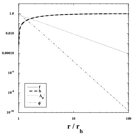
Figure 1: Numerical solutions of $f,h,A_{0}^{\prime},\phi^{\prime}$ outside the event horizon for the cubic coupling $f_{3}=\beta_{3}$ with $\tilde{\beta}_{3}=\beta_{3}M_{\rm pl}/r_{h}^{2}=1.0$ and $\mu=0.5$. Both $A_{0}^{\prime}$ and $\phi^{\prime}$ are normalized by $M_{\rm pl}/r_{h}$. We choose the boundary conditions to be consistent with Eqs. (37)-(39) at $r=1.001r_{h}$.

To confirm the regularity of solutions outside the horizon, we numerically integrate Eqs. (32)-(34) with Eq. (31) by using the boundary conditions (37)-(39) in the vicinity of the horizon. In Fig. 1, we show the integrated solutions of $f,h,A_{0}^{\prime},\phi^{\prime}$ versus $r/r_{h}$ for $\tilde{\beta}_{3}=1.0$ and $\mu=0.5$. They are indeed regular throughout the horizon exterior. The two metric components are close to 0 around $r=r_{h}$ and they asymptotically approach 1 for $r\gg r_{h}$. As estimated by Eqs. (37) and (38), the cubic coupling $\tilde{\beta}_{3}$ induces the difference between $f$ and $h$ mostly around the horizon. In the numerical simulation of Fig. 1, the difference between $f$ and $h$ reaches a maximum close to the order $10^{-2}$ in the vicinity of the horizon and then $|f-h|$ decreases for increasing $r$.

From Eq. (45), the field derivative rapidly decreases as $\phi^{\prime}\propto r^{-5}$ for $r\gg r_{h}$. This decreasing rate is larger than that of the derivative $A_{0}^{\prime}\propto r^{-2}$. Then, $\phi^{\prime}\ll A_{0}^{\prime}$ for $r\gg r_{h}$, but $\phi^{\prime}$ cannot be neglected relative to $A_{0}^{\prime}$ for $r$ closer to $r_{h}$. For $\tilde{\beta}_{3}$ of the order of 1, the value $\phi^{\prime}=4\tilde{\beta}_{3}\mu M_{\rm pl}/r_{h}$ on the horizon becomes comparable to $A_{0}^{\prime}\simeq\sqrt{2\mu}M_{\rm pl}/r_{h}$. Indeed, this property can be confirmed in Fig. 1. Thus, there exists the regular BH solution with a nontrivial scalar hair, whose effect mostly manifests in the nonlinear regime of gravity.

IV Quartic interactions

We proceed to the case of quartic interactions given by the Lagrangian ${\cal L}_{\rm SVT}^{4}$. First of all, we notice that each term in Eq. (18) contains positive powers of $f$ and $h$. Hence, as long as $\phi^{\prime}$ and $A_{0}^{\prime}$ are finite on the horizon, the current $J_{\phi}$ is constrained to be 0. Moreover, except for the term $-2rhA_{0}^{\prime 2}f_{3}$, each term in $J_{\phi}$ is multiplied by the positive powers of $\phi^{\prime}$. This means that, for the theories with $f_{3}=0$, the solution to $J_{\phi}=0$ compatible with the boundary condition $\phi^{\prime}\to 0$ at spatial infinity should correspond to the no scalar-hair solution $\phi^{\prime}=0$ for arbitrary $r$. Then, we need the cubic interaction for the realization of hairy BH solutions with nonvanishing $\phi^{\prime}$. In the following, we consider the model given by the functions

$$f_{2}(X,F)=X+F\,,\qquad f_{3}(X)=\beta_{3}\,,\qquad f_{4}(X)=\beta_{4}X^{n}\,,\qquad\tilde{f}_{4}=0\,,$$ (47)

where $\beta_{3},\beta_{4}$ and $n~{}(\geq 0)$ are constants. For concreteness, we will study the two cases: (i) $n=0$ and (ii) $n=1$, separately.

IV.1 Model with $f_{4}(X)=\beta_{4}$

For the model with $n=0$, the current conservation $J_{\phi}=0$ leads to the relation same as Eq. (31) between $\phi^{\prime}$ and $A_{0}^{\prime}$. On using this relation, Eqs. (14), (15) and (17) reduce, respectively, to

$$M_{\rm pl}^{2}rfh^{\prime} = M_{\rm pl}^{2}f(1-h)-\frac{h}{2f}A_{0}^{\prime 2}\left[fr^{2}+12\beta_{3}^{2}h^{2}A_{0}^{\prime 2}+8\beta_{4}f(1-h)\right]\,,$$ (48)

$$M_{\rm pl}^{2}rhf^{\prime} = M_{\rm pl}^{2}f(1-h)-\frac{h}{2f}A_{0}^{\prime 2}\left[fr^{2}+20\beta_{3}^{2}h^{2}A_{0}^{\prime 2}+8\beta_{4}f(1-3h)\right]\,,$$ (49)

$$A_{0}^{\prime\prime} = -\frac{2[M_{\rm pl}^{2}f^{2}r^{2}+4(1-h)\beta_{3}^{2}fhM_{\rm pl}^{2}A_{0}^{\prime 2}-\beta_{3}^{2}h^{2}r^{2}A_{0}^{\prime 4}-4\beta_{4}M_{\rm pl}^{2}f^{2}(1-h)-8\beta_{3}^{2}\beta_{4}h^{2}(2h+1)A_{0}^{\prime 4}]}{frM_{\rm pl}^{2}[fr^{2}+24\beta_{3}^{2}h^{2}A_{0}^{\prime 2}+8\beta_{4}f(1-h)]}A_{0}^{\prime}\,.$$ (50)

Substituting Eqs. (27) and (36) into Eqs. (48)-(50), the iterative solutions around $r=r_{h}$ up to the order of $(r-r_{h})^{2}$ are given by

$$f = \left(1-\mu\right)\left(\frac{r}{r_{h}}-1\right)-\frac{1-2\mu+12\tilde{\beta}_{3}^{2}\mu^{2}(1-\mu)+4\tilde{\beta}_{4}(24\tilde{\beta}_{4}\mu^{2}-40\tilde{\beta}_{4}\mu+3\mu^{2}+16\tilde{\beta}_{4}-9\mu+4)}{(1+8\tilde{\beta}_{4})^{2}}\left(\frac{r}{r_{h}}-1\right)^{2}\,,$$ (51)

$$h = \left(1-\mu\right)\left(\frac{r}{r_{h}}-1\right)-\frac{1-2\mu-4\tilde{\beta}_{3}^{2}\mu^{2}(1-\mu)-4\tilde{\beta}_{4}(8\tilde{\beta}_{4}\mu^{2}+8\tilde{\beta}_{4}\mu+\mu^{2}-16\tilde{\beta}_{4}+5\mu-4)}{(1+8\tilde{\beta}_{4})^{2}}\left(\frac{r}{r_{h}}-1\right)^{2}\,,$$ (52)

$$A_{0} = a_{0}+\sqrt{\frac{2\mu}{1+8\tilde{\beta}_{4}}}M_{\rm pl}\left(\frac{r}{r_{h}}-1\right)-\sqrt{\frac{2\mu}{(1+8\tilde{\beta}_{4})^{5}}}M_{\rm pl}\left[1+4\tilde{\beta}_{3}^{2}\mu(2-\mu)+4\tilde{\beta}_{4}-32\tilde{\beta}_{4}^{2}\right]\left(\frac{r}{r_{h}}-1\right)^{2}\,,$$ (53)

where $\tilde{\beta}_{4}\equiv\beta_{4}/r_{h}^{2}$. From Eq. (31), the scalar derivative up to the order of $r-r_{h}$ reads

$$\phi^{\prime}=\frac{4\tilde{\beta}_{3}\mu M_{\rm pl}}{r_{h}(1+8\tilde{\beta}_{4})}\left[1-\frac{5+32\tilde{\beta}_{3}^{2}\mu(1-\mu)+16\tilde{\beta}_{4}(2+\mu-4\tilde{\beta}_{4}+8\tilde{\beta}_{4}\mu)}{(1+8\tilde{\beta}_{4})^{2}}\left(\frac{r}{r_{h}}-1\right)\right]\,.$$ (54)

Substituting the large-distance expansions (41) into Eqs. (48)-(50) and setting $\tilde{f}_{1}=\tilde{h}_{1}=-2M$ and $\tilde{a}_{1}=Q$, the iterative solutions at spatial infinity yield

$$f = 1-\frac{2M}{r}+\frac{Q^{2}}{2M_{\rm pl}^{2}r^{2}}-\frac{2\beta_{4}Q^{2}}{M_{\rm pl}^{2}r^{4}}+\frac{2\beta_{4}MQ^{2}}{M_{\rm pl}^{2}r^{5}}-\frac{3\beta_{4}Q^{4}}{5M_{\rm pl}^{4}r^{6}}+\frac{256\beta_{4}^{2}MQ^{2}}{7M_{\rm pl}^{2}r^{7}}$$ (55)

$$+\frac{3Q^{2}(M_{\rm pl}^{2}Q^{2}\beta_{3}^{2}-28\beta_{4}^{2}Q^{2}-256\beta_{4}^{2}M^{2}M_{\rm pl}^{2})}{14M_{\rm pl}^{4}r^{8}}\,,$$

$$h = 1-\frac{2M}{r}+\frac{Q^{2}}{2M_{\rm pl}^{2}r^{2}}-\frac{2\beta_{4}MQ^{2}}{M_{\rm pl}^{2}r^{5}}+\frac{2\beta_{4}Q^{4}}{5M_{\rm pl}^{4}r^{6}}-\frac{2Q^{2}(\beta_{3}^{2}Q^{2}-64\beta_{4}^{2}M^{2})}{7M_{\rm pl}^{2}r^{8}}\,,$$ (56)

$$A_{0} = P+\frac{Q}{r}-\frac{4\beta_{4}MQ}{r^{4}}+\frac{3\beta_{4}Q^{3}}{5M_{\rm pl}^{2}r^{5}}-\frac{8Q(\beta_{3}^{2}Q^{2}-32\beta_{4}^{2}M^{2})}{7r^{7}}+\frac{2MQ^{3}(7\beta_{3}^{2}M_{\rm pl}^{2}-48\beta_{4}^{2})}{7M_{\rm pl}^{2}r^{8}}\,,$$ (57)

$$\phi^{\prime} = \frac{2\beta_{3}Q^{2}}{r^{5}}-\frac{64\beta_{3}\beta_{4}MQ^{2}}{r^{8}}\,,$$ (58)

up to the order of $1/r^{8}$. From the current conservation (17), the $U(1)$ charge $Q$ at spatial infinity is related to the quantities $\mu$ and $r_{h}$ around the horizon as

$$\sqrt{2\mu(r_{h}^{2}+8\beta_{4})}M_{\rm pl}=-Q\,.$$ (59)

In the limit that $\beta_{3}\to 0$ the field derivatives (54) and (58) vanish, so there are no scalar hairs for the theories with $f_{3}=0$. In this case, the large-distance solutions (55)-(57) reduce to those with vector hair obtained by Horndeski in 1978 for the pure $U(1)$-invariant interaction $\beta_{4}L^{\mu\nu\alpha\beta}F_{\mu\nu}F_{\alpha\beta}$ HorndeskiBH . We note that the iterative solutions (51)-(54) around the horizon are also consistent with those derived in Refs. VTastrophys2 . Unlike the solutions at spatial infinity arising from the cubic interaction, the quartic coupling $\beta_{4}$ leads to corrections to $f,h,A_{0}$ at the orders of $1/r^{4},1/r^{5},1/r^{4}$, respectively. In the vicinity of the horizon, the coupling $\beta_{4}$ appears at the orders of $(r-r_{h})^{2}$ in $f,h$ and of $r-r_{h}$ in $A_{0}$.

For $\beta_{3}\neq 0$, the BH solutions derived above contain the nonvanishing scalar hair $\phi^{\prime}$. Besides the quartic coupling $\beta_{4}$, the effects of $\beta_{3}$ on $f,h,A_{0}$ arise at the orders of $(r-r_{h})^{2}$ around $r=r_{h}$, so that $f$ and $h$ are different from each other. Compared to the case $\beta_{4}=0$, the derivative $\phi^{\prime}$ on the horizon is modified by the factor $(1+8\tilde{\beta}_{4})^{-1}$. We have numerically integrated Eqs. (48)-(50) outside the horizon by using Eqs. (51)-(54) as boundary conditions and found that the solutions smoothly connect to the large-distance solutions (55)-(58) for $|\tilde{\beta}_{4}|<{\cal O}(0.1)$. As in the case of Fig. 1, the scalar hair manifests itself mostly in the vicinity of the horizon. Thus, there exist regular BH solutions endowed with both scalar and vector hairs. For $|\tilde{\beta}_{4}|>{\cal O}(0.1)$ the last terms in Eqs. (48) and (49) can be larger than the first terms on their right hand sides, so that the regularity of BH solutions outside the horizon tends to be violated.

IV.2 Model with $f_{4}(X)=\beta_{4}X$

Let us consider the quartic interaction $f_{4}(X)=\beta_{4}X$. From the current conservation $J_{\phi}=0$, it follows that

$$\phi^{\prime}=\frac{2\beta_{3}rhA_{0}^{\prime 2}}{fr^{2}+2\beta_{4}h(2-3h)A_{0}^{\prime 2}}\,,$$ (60)

which does not vanish for $\beta_{3}\neq 0$. The iterative solutions around the horizon expanded up to the order of $(r-r_{h})^{2}$ are given by

$$f = \left(1-\mu\right)\left(\frac{r}{r_{h}}-1\right)-\frac{1-2\mu+12\tilde{\beta}_{3}^{2}\mu^{2}(1-\mu)+8\bar{\beta}_{4}\mu(1-2\mu)}{1+8\bar{\beta}_{4}\mu}\left(\frac{r}{r_{h}}-1\right)^{2}\,,$$ (61)

$$h = \left(1-\mu\right)\left(\frac{r}{r_{h}}-1\right)-\frac{1-2\mu-4\tilde{\beta}_{3}^{2}\mu^{2}(1-\mu)+8\bar{\beta}_{4}\mu(1-2\mu)}{1+8\bar{\beta}_{4}\mu}\left(\frac{r}{r_{h}}-1\right)^{2}\,,$$ (62)

$$A_{0} = a_{0}+\sqrt{2\mu}M_{\rm pl}\left(\frac{r}{r_{h}}-1\right)-\sqrt{2\mu}M_{\rm pl}\frac{1+4\tilde{\beta}_{3}^{2}\mu(2-\mu)+16\bar{\beta}_{4}\mu(1+2\tilde{\beta}_{3}^{2}\mu+4\bar{\beta}_{4}\mu)}{(1+8\bar{\beta}_{4}\mu)^{2}}\left(\frac{r}{r_{h}}-1\right)^{2}\,,$$ (63)

where $\bar{\beta}_{4}\equiv\beta_{4}M_{\rm pl}^{2}/r_{h}^{4}$. From Eq. (60), the scalar derivative up to the order of $r-r_{h}$ yields

$$\phi^{\prime}=\frac{4\tilde{\beta}_{3}\mu M_{\rm pl}}{r_{h}(1+8\bar{\beta}_{4}\mu)}\left[1-\frac{32\tilde{\beta}_{3}^{2}\mu(1-\mu)(1+4\bar{\beta}_{4}\mu)+(1+8\bar{\beta}_{4}\mu)^{2}\{5+4\bar{\beta}_{4}\mu(3\mu-5)\}}{(1+8\bar{\beta}_{4}\mu)^{3}}\left(\frac{r}{r_{h}}-1\right)\right]\,.$$ (64)

At spatial infinity, we find that the solutions to $f,h,A_{0}$ are of the same forms as Eqs. (42)-(44) up to the order of $1/r^{8}$. The scalar derivative $\phi^{\prime}$ also has the same dependence as Eq. (45). Thus, unlike the constant $f_{4}$ model, the coupling $\beta_{4}$ does not appear in the large-distance expansions of $f,h,A_{0},\phi^{\prime}$ at the order lower than $1/r^{8}$. Note that the current conservation (17) gives the relation same as Eq. (46).

Around the horizon, both the couplings $\beta_{3}$ and $\beta_{4}$ appear in Eqs. (61)-(63) at the order of $(r-r_{h})^{2}$. From Eqs. (64), the scalar derivative $\phi^{\prime}$ is comparable to $A_{0}^{\prime}\simeq\sqrt{2\mu}M_{\rm pl}/r_{h}$ for $\tilde{\beta}_{3}/(1+8\bar{\beta}_{4}\mu)$ of the order of unity. Numerically we confirmed that the iterative solutions (61)-(64) can connect to those at spatial infinity without discontinuities. Hence we have the regular BH solutions with the scalar hair manifesting itself in the vicinity of the horizon. We stress that this hairy solution arises by the presence of the cubic coupling $f_{3}=\beta_{3}$ besides the quartic interaction $f_{4}=\beta_{4}X$.

V Conclusions

In this letter, we studied the static and spherically symmetric BH solutions in SVT theories with gauge-invariant derivative scalar-vector interactions and a non-minimal coupling to gravity. The longitudinal mode of the vector field does not propagate due to the $U(1)$ gauge invariance, so we are left with the equations of motion for a scalar field $\phi$ and a temporal vector component $A_{0}$ besides the gravitational equations of two metric components $f$ and $h$. In shift-symmetric theories where the functions $f_{2},f_{3},f_{4},\tilde{f}_{4}$ in the action (11) do not contain any $\phi$ dependence, there is the current conservation $J_{\phi}={\rm constant}$ associated with the scalar $\phi$.

Except for the term $-2rhA_{0}^{\prime 2}f_{3}$ in the square bracket of Eq. (18), the current $J_{\phi}$ contains the products of positive powers of $\phi^{\prime}$ and $f$ or $h$. The regularities of $\phi^{\prime}$ and $A_{0}^{\prime}$ on the horizon lead to $J_{\phi}=0$ in general. Then, in the absence of the term $-2rhA_{0}^{\prime 2}f_{3}$, the solutions consistent with the boundary condition $\phi^{\prime}\to 0$ at spatial infinity correspond to $\phi^{\prime}=0$ for arbitrary radial distance $r$. Existence of the cubic interaction $f_{3}$ breaks this structure and allows the possibility for realizing hairy BH solutions with $\phi^{\prime}\neq 0$.

In the presence of the cubic coupling $f_{3}=\beta_{3}$ besides the function $f_{2}=X+F$, the scalar derivative $\phi^{\prime}$ is related to the temporal vector component in the form (31). We derived the iterative solutions (37)-(40) expanded around the horizon and showed that the cubic coupling $\beta_{3}$ induces corrections to the RN solutions of $f,h,A_{0}$ at the order of $(r-r_{h})^{2}$. In the limit that $r\to r_{h}$, the scalar derivative approaches the nonvanishing finite value $\phi^{\prime}\to 4\tilde{\beta}_{3}\mu M_{\rm pl}/r_{h}$. At spatial infinity, the cubic coupling $\beta_{3}$ gives rise to corrections to $f,h,A_{0}^{\prime}$ at the order of $1/r^{8}$. In this region, the scalar derivative quickly decreases as $\phi^{\prime}\simeq 2\beta_{3}Q^{2}/r^{5}$, but the scalar hair manifests itself around the horizon. Numerically, we confirmed the regularity of hairy BH solutions throughout the horizon exterior, see Fig. 1. From the current conservation $J_{A}={\rm constant}$, the $U(1)$ charge $Q$ at spatial infinity is related to the quantities $\mu$ and $r_{h}$ around the horizon according to Eq. (46).

We also studied the cases in which the quartic interactions $f_{4}=\beta_{4}X^{n}$ with $n=0$ or $n=1$ are present besides the cubic coupling $f_{3}=\beta_{3}$. In the limit that $\beta_{3}\to 0$, the model with $f_{4}=\beta_{4}$ recovers BH solutions with vector hair discussed by Horndeski in 1978. Existence of the cubic coupling $\beta_{3}$ leads to a new hairy BH solution endowed with both scalar and vector hairs. For the quartic interaction $f_{4}=\beta_{4}X$, we also showed the presence of a hairy BH solution where the effects of couplings $\beta_{3}$ and $\beta_{4}$ on $f,h,A_{0}^{\prime},\phi^{\prime}$ manifests themselves in the vicinity of the horizon.

In this letter, we showed the existence of hairy BH solutions induced by the scalar-vector interaction in $U(1)$ gauge-invariant SVT theories as a first step, but it is of interest to study what happens for the SVT theories with the broken gauge invariance. Moreover, the application of gauge-broken SVT theories to cosmology will be interesting in connection to the problems of inflation, dark energy, and dark matter. These topics are left for future works.

References

• (1) E. J. Copeland, M. Sami and S. Tsujikawa, Int. J. Mod. Phys. D 15, 1753 (2006) [hep-th/0603057]; T. P. Sotiriou and V. Faraoni, Rev. Mod. Phys.  82, 451 (2010) [arXiv:0805.1726 [gr-qc]]; A. De Felice and S. Tsujikawa, Living Rev. Rel.  13, 3 (2010) [arXiv:1002.4928 [gr-qc]]; T. Clifton, P. G. Ferreira, A. Padilla and C. Skordis, Phys. Rept.  513, 1 (2012) [arXiv:1106.2476 [astro-ph.CO]]; L. Amendola et al. [Euclid Theory Working Group], Living Rev. Rel.  16, 6 (2013) [arXiv:1206.1225 [astro-ph.CO]]; L. Amendola et al. [Euclid Theory Working Group], arXiv:1606.00180 [astro-ph.CO]; A. Joyce, B. Jain, J. Khoury and M. Trodden, Phys. Rept.  568, 1 (2015) [arXiv:1407.0059 [astro-ph.CO]]; P. Bull et al., Phys. Dark Univ.  12, 56 (2016) [arXiv:1512.05356 [astro-ph.CO]].
• (2) G. W. Horndeski, Int. J. Theor. Phys.  10, 363 (1974).
• (3) C. Deffayet, X. Gao, D. A. Steer and G. Zahariade, Phys. Rev. D 84, 064039 (2011) [arXiv:1103.3260 [hep-th]]; T. Kobayashi, M. Yamaguchi and J. ’i. Yokoyama, Prog. Theor. Phys.  126, 511 (2011) [arXiv:1105.5723 [hep-th]]; C. Charmousis, E. J. Copeland, A. Padilla and P. M. Saffin, Phys. Rev. Lett.  108, 051101 (2012) [arXiv:1106.2000 [hep-th]].
• (4) G. W. Horndeski, J. Math. Phys.  17, 1980 (1976).
• (5) L. Heisenberg, JCAP 1405, 015 (2014) [arXiv:1402.7026 [hep-th]].
• (6) J. Beltran Jimenez and L. Heisenberg, Phys. Lett. B 757, 405 (2016) [arXiv:1602.03410 [hep-th]].
• (7) G. Tasinato, JHEP 1404, 067 (2014) [arXiv:1402.6450 [hep-th]]; G. Tasinato, Class. Quant. Grav.  31, 225004 (2014) [arXiv:1404.4883 [hep-th]]. E. Allys, P. Peter and Y. Rodriguez, JCAP 1602, 004 (2016) [arXiv:1511.03101 [hep-th]]; L. Heisenberg, R. Kase and S. Tsujikawa, Phys. Lett. B 760, 617 (2016) [arXiv:1605.05565 [hep-th]]; R. Kimura, A. Naruko and D. Yoshida, JCAP 1701, 002 (2017) [arXiv:1608.07066 [gr-qc]]; L. Heisenberg, arXiv:1705.05387 [hep-th].
• (8) J. D. Barrow, M. Thorsrud and K. Yamamoto, JHEP 1302 (2013) 146 [arXiv:1211.5403 [gr-qc]]; J. Beltran Jimenez, R. Durrer, L. Heisenberg and M. Thorsrud, JCAP 1310, 064 (2013) [arXiv:1308.1867 [hep-th]]; M. Hull, K. Koyama and G. Tasinato, Phys. Rev. D 93, 064012 (2016) [arXiv:1510.07029 [hep-th]].
• (9) A. De Felice, L. Heisenberg, R. Kase, S. Mukohyama, S. Tsujikawa and Y. l. Zhang, JCAP 1606, 048 (2016) [arXiv:1603.05806 [gr-qc]]; A. De Felice, L. Heisenberg, R. Kase, S. Mukohyama, S. Tsujikawa and Y. l. Zhang, Phys. Rev. D 94, 044024 (2016) [arXiv:1605.05066 [gr-qc]]; L. Heisenberg, R. Kase and S. Tsujikawa, JCAP 1611, 008 (2016) [arXiv:1607.03175 [gr-qc]]; A. De Felice, L. Heisenberg and S. Tsujikawa, Phys. Rev. D 95, 123540 (2017) [arXiv:1703.09573 [astro-ph.CO]].
• (10) A. De Felice, L. Heisenberg, R. Kase, S. Tsujikawa, Y. l. Zhang and G. B. Zhao, Phys. Rev. D 93, 104016 (2016) [arXiv:1602.00371 [gr-qc]]; S. Nakamura, R. Kase and S. Tsujikawa, Phys. Rev. D 96, 084005 (2017) [arXiv:1707.09194 [gr-qc]].
• (11) J. Chagoya, G. Niz and G. Tasinato, Class. Quant. Grav.  33, no. 17, 175007 (2016) [arXiv:1602.08697 [hep-th]]; Z. Y. Fan, JHEP 1609, 039 (2016) [arXiv:1606.00684 [hep-th]]; M. Minamitsuji, Phys. Rev. D 94, 084039 (2016) [arXiv:1607.06278 [gr-qc]]; A. Cisterna, M. Hassaine, J. Oliva and M. Rinaldi, Phys. Rev. D 94, 104039 (2016). [arXiv:1609.03430 [gr-qc]]; E. Babichev, C. Charmousis and M. Hassaine, JHEP 1705, 114 (2017) [arXiv:1703.07676 [gr-qc]]; J. Chagoya, G. Niz and G. Tasinato, Class. Quant. Grav.  34, no. 16, 165002 (2017) [arXiv:1703.09555 [gr-qc]].
• (12) L. Heisenberg, R. Kase, M. Minamitsuji and S. Tsujikawa, Phys. Rev. D 96, 084049 (2017) [arXiv:1705.09662 [gr-qc]]; L. Heisenberg, R. Kase, M. Minamitsuji and S. Tsujikawa, JCAP 1708, 024 (2017) [arXiv:1706.05115 [gr-qc]].
• (13) R. Kase, M. Minamitsuji and S. Tsujikawa, arXiv:1711.08713 [gr-qc]; R. Kase, M. Minamitsuji, S. Tsujikawa and Y. l. Zhang, JCAP 1802, 048 (2018) [arXiv:1801.01787 [gr-qc]].
• (14) L. Heisenberg, arXiv:1801.01523 [gr-qc].
• (15) B. P. Abbott et al. [LIGO Scientific and Virgo Collaborations], Phys. Rev. Lett.  116, 061102 (2016) [arXiv:1602.03837 [gr-qc]].
• (16) B. P. Abbott et al. [LIGO Scientific and Virgo Collaborations], Phys. Rev. Lett.  119, 161101 (2017) [arXiv:1710.05832 [gr-qc]].
• (17) P. Channuie and D. Momeni, arXiv:1802.03672 [gr-qc].
• (18) S. W. Hawking, Commun. Math. Phys.  25, 167 (1972); J. D. Bekenstein, Phys. Rev. D 51, R6608 (1995).
• (19) L. Hui and A. Nicolis, Phys. Rev. Lett.  110, 241104 (2013) [arXiv:1202.1296 [hep-th]].
• (20) T. P. Sotiriou and V. Faraoni, Phys. Rev. Lett.  108, 081103 (2012) [arXiv:1109.6324 [gr-qc]]; M. Rinaldi, Phys. Rev. D 86, 084048 (2012) [arXiv:1208.0103 [gr-qc]]; A. Anabalon, A. Cisterna and J. Oliva, Phys. Rev. D 89, 084050 (2014) [arXiv:1312.3597 [gr-qc]]; M. Minamitsuji, Phys. Rev. D 89, 064017 (2014) [arXiv:1312.3759 [gr-qc]]; T. P. Sotiriou and S. Y. Zhou, Phys. Rev. Lett.  112, 251102 (2014) [arXiv:1312.3622 [gr-qc]]; E. Babichev and C. Charmousis, JHEP 1408, 106 (2014) [arXiv:1312.3204 [gr-qc]]; T. Kolyvaris, G. Koutsoumbas, E. Papantonopoulos and G. Siopsis, JHEP 1311, 133 (2013) [arXiv:1308.5280 [hep-th]]; C. Charmousis, T. Kolyvaris, E. Papantonopoulos and M. Tsoukalas, JHEP 1407, 085 (2014) [arXiv:1404.1024 [gr-qc]].
• (21) G. W. Horndeski, Phys. Rev. D 17, 391 (1978).