Monte-Carlo simulations of the detailed iron absorption line profiles from thermal winds in X-ray binaries

Abstract

Blue–shifted absorption lines from highly ionised iron are seen in some high inclination X-ray binary systems, indicating the presence of an equatorial disc wind. This launch mechanism is under debate, but thermal driving should be ubiquitous. X-ray irradiation from the central source heats disc surface, forming a wind from the outer disc where the local escape velocity is lower than the sound speed. The mass loss rate from each part of the disc is determined by the luminosity and spectral shape of the central source. We use these together with an assumed density and velocity structure of the wind to predict the column density and ionisation state, then combine this with a Monte-Carlo radiation transfer to predict the detailed shape of the absorption (and emission) line profiles. We test this on the persistent wind seen in the bright neutron star binary GX 13+1, with luminosity $L/L_{\mathrm{Edd}}\sim 0.5$. We approximately include the effect of radiation pressure because of high luminosity, and compute line features. We compare these to the highest resolution data, the Chandra third order grating spectra, which we show here for the first time. This is the first physical model for the wind in this system, and it succeeds in reproducing many of the features seen in the data, showing that the wind in GX13+1 is most likely a thermal-radiation driven wind. This approach, combined with better streamline structures derived from full radiation hydrodynamic simulations, will allow future calorimeter data to explore the detail wind structure.

1 Introduction

Low Mass X-ray Binaries (LMXBs) are systems where a companion star overflows its Roche lobe, so that material spirals down towards a compact object which can be either a black hole or neutron star. The observed X-ray emission is powered by the enourmous gravitational potential energy released by this material as it falls inwards, lighting up the regions of intense space–time curvature and giving observational tests of strong gravity.

This inflow also powers outflows. Accretion disc winds are seen via blue–shifted absorption lines from highly ionised material in high inclination LMXBs (see e.g. the reviews by Ponti et al. 2012; Díaz Trigo & Boirin 2016) but the driving mechanism of these winds is not well understood. The potential candidates are acceleration of gas by the Lorentz force from magnetic fields threading discs (magnetic driving: Blandford & Payne 1982; Fukumura et al. 2014), radiation pressure on the electrons (continuum driving: Proga & Kallman 2002; Hashizume et al. 2015) and thermal expansion of the hot disc atmosphere heated by the central X-ray source, which makes a wind at radii which are large enough for the sound speed to exceed the local escape velocity (thermal driving: Begelman et al. 1983; Woods et al. 1996, hereafter W96).

Recent work has focussed on magnetic driving, primarily because of a single observation of dramatic wind absorption seen from the black hole GRO J1655-40 at low luminosity, far below the Eddington limit where continuum driving becomes important, and with a derived launch radius which is far too small for thermal driving (Miller et al., 2006; Luketic et al., 2010; Higginbottom & Proga, 2015). Magnetic wind models can fit this spectrum (Fukumura et al., 2017), but then it is difficult to understand why such high column and (relatively) low ionisation winds are not seen from other observations of this object or any other high inclination systems with similar luminosities and spectra. Instead, the unique properties of this wind could potentially be explained if the outflow has become optically thick along the line of sight. This would suppress the observed flux from an intrinsically super–Eddington source (Shidatsu et al., 2016; Neilsen et al., 2016). Alternatively, this singular wind may be a transient phenomena, not representative of the somewhat lower column/higher ionisation winds which are normally seen.

What then powers the more typical winds? Thermal driving qualitatively fits the observed properties, as these winds are preferentially seen in systems with larger discs (Díaz Trigo & Boirin, 2016). X-rays from near the compact objects (the inner disc emission and any corona and/or boundary layer) irradiate the outer disc, and the balance between Compton heating and cooling heats the surface to the Compton temperature, which is a luminosity weighted mean energy given by $T_{\mathrm{IC}}=\frac{1}{4}\int EL(E)dE/\int L(E)dE$ (Begelman et al. 1983; Done et al. 2018, hereafter D18).This temperature is constant with radius, as it depends only on the spectrum of the radiation from the central region, but gravity decreases with distance from the source. For a large enough disc, the isothermal sound speed from this Compton temperature is bigger than the escape velocity, so the heated material makes a transition from forming a bound atmosphere, to an outflowing wind. This defines the Compton Radius ($R_{\mathrm{IC}}=GMm_{p}/kT_{\mathrm{IC}}=(6.4\times 10^{4}/T_{\mathrm{IC,8}})R_{g}$, where $R_{g}=GM/c^{2}$ and $T_{\mathrm{IC,8}}=T_{\mathrm{IC}}/10^{8}~{}K$) as the typical launch radius for a thermal wind (Begelman et al. 1983, D18).

These thermal wind models give an analytic solution for the mass loss rate from the disc (Begelman et al. 1983, W96). However, to calculate the observables such as column density and ionisation structure requires an understanding of the velocity as a function of two-dimensional position (or equivalently, velocity as a function of length along a streamline, together with the shape of the streamlines). D18 assume a very simple 2-dimensional density and velocity structure along radial streamlines, and show that this can match the column seen in the full hydrodynamic simulation of W96. This composite model was applied to multiple spectra of H1743–322, matching the wind seen in its disk dominated state, and predicting the disappearance of these wind absorption lines in a bright low/hard state, as observed (Shidatsu & Done 2017, in prep). This wind disappearance does not occur from simply the change in photo-ionisation state from the changing illumination (Miller et al., 2012). The key difference is that thermal winds respond to changing illumination by changing their launch radius, density and velocity as well as responding to the changing photo-ionising spectrum (Shidatsu & Done 2017, in prep).

Here we explore the thermal wind predictions in more detail, using a 3–dimensional Monte-Carlo simulation code MONACO (Odaka et al., 2011) to calculate the radiation transport through the material so as to predict the resulting emission and absorption line profiles. We calculate these for the very simple constant velocity structure assumed in D18, and then extend this to consider an accelerating wind along biconical streamlines, as a more appropriate disk wind geometry (Waters & Proga, 2012). We show results from both these geometries for the specific case of $L/L_{\mathrm{Edd}}=0.3,T_{\mathrm{IC,8}}=0.13,R_{out}=5R_{\mathrm{IC}}$ to compare with W96.

We apply the biconical wind model to the bright neutron star binary system GX13+1. This system is unique amongst all the black hole and neutron star binaries in showing persistently strong blueshifted absorption features in its spectrum (Ueda et al., 2004; D’Aì et al., 2014). The X-ray continuum is rather stable, with $T_{\mathrm{IC,8}}\sim 0.13$, making it a good match to the simulations, but it has slightly higher luminosity at $L/L_{\mathrm{Edd}}=0.5$. This means that radiation pressure should become important, decreasing the radius from which the wind can be launched and increasing its column density. We compare results from a hybrid thermal/radiative wind (calculated using the approximate radiation pressure correction from D18) to the detailed absorption line profiles seen in the third order Chandra grating data from this source. This is the first quantatiative, physical model for the wind, and the first exploration of the highest spectral resolution data from this source. While magnetic driving models are always possible, our results match the majority of the observed features, showing that the wind properites are broadly consistent with hybrid thermal-radiative driving.

2 Radiative Transfer Code

We use the Monte-Carlo simulation code MONACO (Odaka et al., 2011) to calculate radiative transfer through the wind. MONACO uses its original physics implementation of photon interactions (Watanabe et al., 2006; Odaka et al., 2011) while it employs the Geant4 toolkit library (Agostinelli et al., 2003) for photon tracking in an arbitrary 3–dimensional geometry.

We consider an azimuthally symmetric density and velocity field, then use the XSTAR photo-ionization code (Kallman & Bautista, 2001) to calculate the equilibrium population of ions from each element assuming one-dimensional radiation transfer from the central source. We grid in radial distance, $r$, and $\theta$ and assume the illuminating flux is the transmitted part of the central spectrum along the line of sight to the element. This gives an ionisation parameter

$$\xi(r,\theta)=\frac{L\exp(-\tau_{abs})}{n(r,\theta)r^{2}}$$ (2.1)

where $\tau_{abs}$ is the optical depth to absorption (but does not include electron scattering), and $n(r,\theta)$ is the density as a function of position.

We then use MONACO to track photons through this ionisation structure, including their interaction with this material. Photons interacting with ions can be absorbed in photo-ionisation or photo-excitation, and photons generated via recombination and atomic deexcitation are tracked. Doppler shifts of the absorption cross-sections from the velocity structure of the material are included, as is the Compton energy change on interaction with free electrons. Ideally, this calculated radiation field should then be used as input to XSTAR, the ion populations recalculated, and the process should be iterated until convergence. However, for our simulations here the wind is mostly optically thin, so we do not include this self-consistent iteration. This method of radiation transfer calculation is based on the Hagino et al. (2015), but the geometry and the velocity/density structure we use is reflected on the thermally driven winds in LMXBs whereas Hagino et al. (2015) is focussed on the UV-line driven winds in Active Galactic Nucleus (AGN). Also, as thermal winds are typically highly ionised, we consider only H-like and He-like ions of Fe and calculate the spectrum only over a restricted energy band of 6.5–7.2 keV. Table.1 details the transitions used.

Line ID	Energy [keV]	oscillator strength
Fe XXV He$\alpha~{}\mathrm{y}$	6.668	$6.57\times 10^{-2}$
Fe XXV He$\alpha~{}\mathrm{w}$	6.700	$7.26\times 10^{-1}$
Fe XXVI Ly$\alpha_{2}$	6.952	$1.36\times 10^{-1}$
Fe XXVI Ly$\alpha_{1}$	6.973	$2.73\times 10^{-1}$

Table 1: Detailed parameters for each line included in these MONACO simulations. Note that we list only lines which have larger oscillator strengths than $10^{-3}$.

3 Radial streamlines: D18

3.1 Geometry and Parameters

We first consider the radial streamline wind model of D18. This calculates the analytic mass loss rate per unit area, $\dot{m}(R)$ where $R$ denotes distance along the disc plane. Integrating over the whole disc gives the total mass loss rate in the wind, $\dot{M}$. This is assumed to flow along radial (centered at the origin) streamlines from a launch radius which is $0.2R_{\mathrm{IC}}$ for high $L/L_{\mathrm{Edd}}$, with constant velocity set at the mass loss weighted average escape velocity. The mass loss rate along each radial streamline is weighted with angle such that $\dot{M}(\theta)\propto\dot{M}(1-\cos\theta)$, and then mass conservation gives $n(r,\theta)\propto(1-\cos\theta)/r^{2}$. D18 show that these assumptions lead to a total column density through the structure which matches to within a factor 2 of that in the hydrodynamic simulations of W96 (see also Section 4).

We put this structure into MONACO for $L=0.3L_{\mathrm{Edd}}$ with $T_{\mathrm{IC}}=1.3\times 10^{7}$ K and $R_{\mathrm{out}}=5R_{\mathrm{IC}}$ (mass loss rate $\dot{M}_{w}=2.0\times 10^{19}\mathrm{g~{}s^{-1}}$ for a $10M_{\odot}$ black hole which means the ratio of mass loss rate to mass accretion rate $\dot{M}_{w}/\dot{M}_{a}=3.9$, where the $\dot{M}_{a}=L/(0.1c^{2})$, launch radius of $0.2R_{\mathrm{IC}}\approx 10^{5}R_{g}$ and weighted average $v_{\mathrm{out}}=420\mathrm{km/s}$). We include turbulence, assuming $v_{\mathrm{turb}}=v_{\mathrm{out}}$, and calculate the rotation velocity along each stream line assuming angular momentum conservation (see Appendix A).

We make a grid which follows the symmetry of the assumed structure, i.e. centred on the origin, with 20 linearly spaced spherical shells from $0.2-5R_{\mathrm{IC}}$, and 20 angles, linearly spaced in $\theta$ from $7-83^{\circ}$ (see below). This density structure is shown in the left panel of Fig. 1, while the right panel shows the mean Fe ion state obtained from the XSTAR calculation. This is constant along each streamline because the ionisation parameter $\xi=L/(nr^{2})$, and the constant velocity radial streamlines mean that density decreases as $1/r^{2}$. Fe is almost completely ionised over the whole grid, with a small fraction of hydrogen-like iron remaining only for high inclination streamlines.

Figure 1: Distribution of density (left) and mean Fe ionization state (right) for the radial streamline model

3.2 MONACO output

Fig. 2 shows the resulting spectra at three different inclination angles. These show that the emission lines are always similarly weak, and that the electron scattered continuum flux makes only a $\sim 0.5$% contribution to the total flux, but that the absorption lines strongly increase at higher inclination angles. We calculate the equivalent width (EW) of each emission and absorption line by fitting the continuum outside the emission and absorption regions with an arbitrary function ($F(E)=aE^{bE+c}$ Odaka et al. 2016). The EW of each emission and absorption line is then measured by numerical integration of the difference between the model and the simulation data. The left panel of Fig. 3 shows the EW of the He-like (red) and H-like Ly$\alpha_{2}$ (green) and Ly$\alpha_{1}$ (blue) absorption lines. The corresponding emission lines always have EW lower than $0.1$ eV so are not seen on this plot. The strong increase of the absorption line EW with inclination clearly shows that the wind is equatorial (by construction from the $1-\cos\theta$ density dependence and constant velocity assumptions). At inclinations above $70^{\circ}$, the Doppler wings of the K$\alpha_{1}$ and K$\alpha_{2}$ absorption lines merge together due to the turbulent velocities, so Fig. 3 shows only a single EW for this blend.

Fig. 3 (right) shows the outflow velocity, as measured from the energy of the deepest absorption lines (with error set by the resolution of the simulation to $\pm 0.5$ eV). These velocities are constant within 25 % as a function of inclination, again by construction due to the assumption of constant radial velocity along radial streamlines.

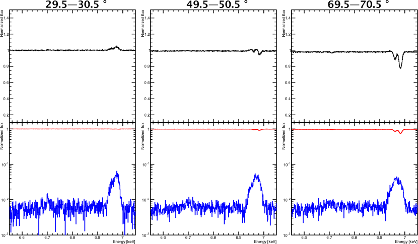
Figure 2: Spectra computed for the radial streamline model with 1 eV resolution for different lines of sight. Each panel shows the spectrum in a different inclination angle bin (the angular bin sizes are indicated the top of each panel). The total spectrum is shown in black (top), the spectrum direct photons in red and scattered/reprocessed spectrum is blue (bottom). Note that the vertical axis is plotted linearly in the top panels but logarithmically in the bottom panels. Lines are Fe XXV  (6.668 keV for $\mathrm{He\alpha}~{}y$ and 6.700 keV for $\mathrm{He\alpha}~{}w$ ) and Fe XXVI  (6.952 keV for $\mathrm{Ly\alpha_{2}}$ and 6.973 keV for $\mathrm{Ly\alpha_{1}})$. The equatorial density structure of the wind means that the absorption is much stronger at high inclination angles. The emission is more isotropic, so it can clearly be seen at low inclination angles, but is absorbed by the wind at high inclinations.

Figure 3: Left panel: EW of the absorption lines as a function of inclination angle, Fe XXV ($\mathrm{He\alpha~{}w}$, red) and Fe XXVI ($\mathrm{Ly\alpha_{2}}$, green and $\mathrm{Ly\alpha_{1}}$, blue). The EW of all absorption lines increases strongly at higher inclination, showing the assumed equatorial disc wind geometry. The Doppler wings (with width set by turbulent velocity) of the two H-like absorption lines start to merge for inclinations above $70^{\circ}$ so above this we show the total EW of the two lines. Right panel: the blue shifted absorption line velocity for each ion species. This clearly shows the assumed constant velocity structure of the radial streamline.

4 Diverging wind

In section 3, we considered a wind model with constant velocity along radial streamlines. However, the expected thermal wind geometry is instead much more like an accelerating, diverging biconical wind Waters & Proga (2012). Full streamline structures which give the density and velocity of the wind at all points can only be found by hydrodynamic calculations (but see Clarke & Alexander 2016 for some analytic approximations). Since modern calculations only exist for the singular case of GRO J1655-40, we follow D18 and use the W96 simulation results. W96 does not give full density/velocity structures, but do give total column density through the wind at three different luminosities. We use these to match to our assumed streamline and velocity structure, which is the standard biconical diverging disc wind used in a variety of systems including cataclysmic variables (Knigge et al., 1995; Long & Knigge, 2002) and Active Galaxies (Sim et al., 2010; Hagino et al., 2015).

4.1 Geometry and Parameters

The geometry can be defined by 3 parameters (Fig. 4).

1. $R_{\mathrm{in}}=0.1R_{\mathrm{IC}}$, the distance from the source to the inner edge of the wind

2. $R_{\mathrm{out}}$, the distance from the source to outer edge of the wind

3. $\alpha_{\mathrm{min}}$, the angle from z axis to the inner edge of the wind

The disc wind is fan-shaped, with a focal point offset down from the centre by a distance $d=0.1R_{\mathrm{IC}}/\tan\alpha_{\mathrm{min}}$ so that the wind fills the angles from $\alpha_{\mathrm{max}}-\alpha_{\mathrm{min}}$ down to the disc surface. We use $R$ to denote distance along the disc surface, and $r,\theta$ denote radial distance and polar angle from the origin, as before. $\alpha_{\mathrm{min}}$ (or equivalently $d$) is a free parameter, which sets the wind geometry.

Streamlines are assumed to be along lines of constant angle $\alpha$ (where $\alpha_{\mathrm{min}}<\alpha<\alpha_{\mathrm{max}}$) from the focal point. Distance along a streamline which starts on the disc at radius $R$ is $l(R)$ (see Appendix. A). Velocity along the streamline is assumed to be of the form $v(r,\theta)=f_{v}c_{ch}(r)\sqrt{\frac{l(r,\theta)}{R(r)}}$, i.e. this wind accelerates with distance along the streamline, with a terminal velocity which is related via a free parameter $f_{v}$ to the characteristic sound speed $c_{ch}$, given by the balance between heating and cooling in the time it takes the wind to reach a height $H\sim R$ (D18). The density structure is solved by the mass conservation continuity equation along streamlines (see Appendix B). We calculate the wind properties out to a distance which is twice that of the focal point of the wind to $R_{\mathrm{out}}$.

We set the free parameter values, $f_{v}$ and $\alpha_{\mathrm{min}}$, and calculate the total column along each line of sight, $N_{H}(\theta)$, to the central source for parameters matching to the three W96 simulations. These are $L/L_{\mathrm{Edd}}=0.3,0.08$ with $R_{\mathrm{out}}=5R_{\mathrm{IC}}$ and $L/L_{\mathrm{Edd}}=0.01$ with $R_{\mathrm{out}}=12R_{\mathrm{IC}}$. We adjust $f_{v}$ and $\alpha_{\mathrm{min}}$ to minimise the difference between our model and W96. We find $\alpha_{\mathrm{min}}=7^{\circ}$ and $f_{v}=0.25$ matches within a factor 2 of the results from W96. Fig. 5 shows results with these parameters (filled circles), compared to the radial wind model of Section 3 (open circles) as well as the W96 results (solid line). This more physically realistic geometry and velocity gives a similarly good match to the simulations as the D18 radial wind.

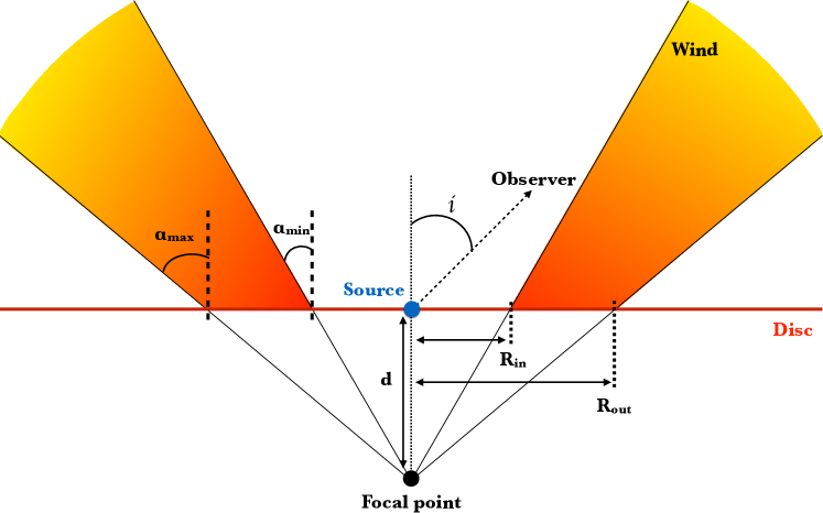
Figure 4: The geometry of the diverging biconical wind model.

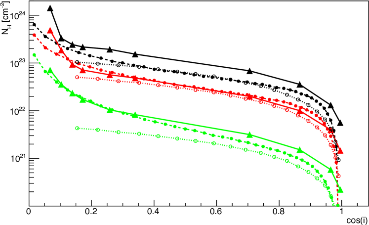
Figure 5: The solid lines show column density as a function of the cosine of the inclination angle through the wind resulting from the hydrodynamic simulations of W96 for $L/L_{\mathrm{Edd}}=$ 0.01(green), 0.08 (red), 0.3 (black). The filled circles show that resulting from the diverging biconical wind (Section 4) while the open circles show the radial streamline model of D18 (Section 3).

The resulting density structure from this different geometry and velocity are shown in the left panel of Fig. 6 for $L/L_{\mathrm{Edd}}=0.3$. Comparing this with the radial wind shows that the density is higher closer to the disc, and lower further away due to the material accelerating away from the disc rather than being at constant velocity. We run XSTAR as before, and the right panel of Fig. 6 shows that this leads to a lower mean ionisation state of Fe than before, and this is no longer constant along the radial sightline due to the different wind geometry.

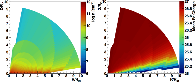
Figure 6: Distribution of density (left) and Fe ionisation state (right) for the diverging wind geometry. The accelerating flow gives higher density material close to the disc compared to the constant velocity outflow model in Fig. 1, giving lower mean ionisation state.

4.2 MONACO output

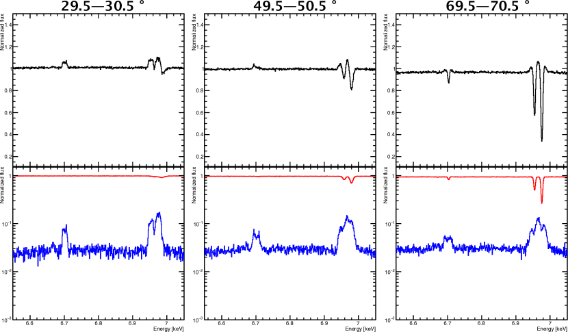
Figure 7: As in Fig 2, but for the diverging biconical wind geometry.

Figure 8: As in Fig. 3, but for the diverging wind model. The lower The lower ionisation state means that there is also a contribution from the intercombination line of Fe XXV $\mathrm{He\alpha~{}y}$ (black) at the highest inclinations.

We calculate the emission and absorption lines resulting from the different wind structure (Fig. 7). The diverging bipolar wind has higher density material closer to the source compared to the radial wind geometry, so it subtends a larger solid angle to scattering. This means that there is more emission line contribution, as well as a higher fraction of electron scattered continuum (around 2%, see the lower panel of Fig. 7). The left panel of Fig. 8 shows the emission line EW (dotted lines) for each ion species (red: Fe XXV w, green: Fe XXVI Ly$\alpha_{2}$, blue: Ly$\alpha_{1}$). These can now be of order 1eV for face on inclinations, decreasing at higher inclination as they are significantly suppressed by line absorption.

The corresponding absorption line EWs are shown as the solid lines (compare to Fig. 3). The lower mean ionisation state leads to more He-like Fe, so there is more of this ion seen in absorption than in the radial streamline model. These absorption lines increase as a function of inclination angle as before, but now the Ly$\alpha_{1}$ and Ly$\alpha_{2}$ do not merge together at the highest inclination angles due to the different velocity structure (see right panel of Fig. 8). The lines are formed preferentially in the higher density material close to the disc. The assumed acceleration law means that the typical velocities here are lower than in the constant velocity model, as the material has only just begun to accelerate. Thus the turbulence is also lower, so the Doppler width of the absorption lines is smaller. This also means that the absorption line saturates to a constant EW at lower column density, so the EW of the absorption lines does not increase so strongly as before at the highest inclination angles.

5 Comparison with GX13+1

We now use the more physically motivated diverging biconical wind geometry to compare with observational data. An ideal source would be one which is not too different from the parameters simulated in the previous sections, as here we know the total column from W96 and know that our assumed velocity/density matches to this. Of the sources listed in Díaz Trigo & Boirin (2016), the neutron star LMXB GX13+1 is the source which has most similar $L/L_{\mathrm{Edd}}$ and $T_{\mathrm{IC}}$ to that assumed here, and it also has the advantage that it is a persistent source, with relatively constant luminosity and spectral shape, and it shows similarly strong absorption lines in multiple datasets.

5.1 Observational data

GX13+1 was observed by the Chandra HighEnergy Transmission Grating (HETG) 4 times in two weeks in 2010 (Table. 2). The first order data are shown in D’Aì et al. (2014) and reveal multiple absorption features from highly ionised elements (see also Ueda et al. 2004 for similar features in an earlier observation). Higher order grating spectra give higher resolution, as demonstrated for the black hole binaries by (Miller et al., 2015). Here we show for the first time the third order Chandra data for GX13+1. We extract first- and third-order HEG spectra from these observations, using CIAO version 4.9 and corresponding calibration files. We reprocess the event files with $"\mathrm{chandra\_repro}"$, and make response files using $"\mathrm{mktgres}"$ to make the redistribution and ancillary response files. We run $"\mathrm{tgsplit}"$ to get the HEG $\pm 3$ spectra, and run $"\mathrm{combine\_grating\_spectra}"$ to combine HEG plus and minus orders for each observation to derive a single 1st order spectrum (black), and a single 3rd order spectrum (red) as shown in Fig. 9. The 1st order spectra can resolve the components of the He-like Fe triplet, with a clear dip to the low energy side at the resonance line energy of 6.7 keV, but the H-like Ly$\alpha_{1}$ and $\alpha_{2}$ are blended together. The higher resolution of the 3rd order spectra is able to clearly separate the He-like intercombination and resonance lines, and even the H-like Ly$\alpha_{1}$ and $\alpha_{2}$ (Miller et al., 2015).

OBSID	MODE	Date	Exposure (ks)
11815	TE-F	24/07/2010	28
11816	TE-F	30/07/2010	28
11814	TE-F	01/08/2010	28
11817	TE-F	03/08/2010	28

Table 2: List of the Chandra HETG observations

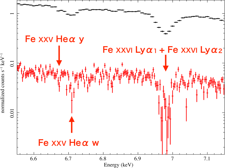
Figure 9: HEG spectra of GX 13+1 from 1st order (black) and 3rd order (red).

5.2 Model of GX 13+1

We fit the contemporaneous RXTE spectrum (ObsID 95338-01-01-05) with a model consisting of a disc, Comptonised boundary layer and its reflection. The resulting inverse Compton temperature of the continuum (disc plus Comptonisation) is $T_{\mathrm{IC}}\sim 1.2\times 10^{7}~{}\mathrm{K}$, almost identical to the simulation (see also D’Aì et al. 2014). The luminosity is $L=0.5L_{\mathrm{Edd}}$ (Díaz Trigo et al., 2014; D’Aì et al., 2014), similar to the maximum simulation value of $L=0.3L_{\mathrm{Edd}}$ in W96. The simulation also requires $R_{\mathrm{out}}$, which can be calculated from the orbital period and mass of binary stars. GX 13+1 has 24 day orbital period, and the neutron star and companion have masses of $1.4M_{\odot}$ and $5M_{\odot}$ respectively (Bandyopadhyay et al., 1999; Corbet et al., 2010). This gives a binary separation $a=4.6\times 10^{12}\mathrm{cm}$, for a Roche-lobe radius $R_{R}/a=0.27$. The disc size is then $R_{\mathrm{out}}=10R_{\mathrm{IC}}$ assuming that $R_{\mathrm{out}}=0.8R_{R}$ (Shahbaz et al., 1998), double the value assumed in the simulations. D18 shows that this increase in disc size makes the predicted column slightly larger, but the effect is fairly small (Fig. 3: D18). Fig. 10 (blue line) shows the predicted column density through the wind as a function of inclination angle. This is very similar to the column predicted for the fiducial simulations (Fig. 5)

However, D18 show that radiation pressure should make a rapidly increasing contribution to the wind as $L/L_{\mathrm{Edd}}$ increases from $0.3-0.7$. The GX13+1 luminosity is midway between these two, so radiation pressure should significantly lower the effective gravity, meaning that the wind can be launched from smaller radii. We follow D18 and estimate a radiation pressure correction to the launch radius of $\bar{R}_{\mathrm{IC}}=(1.0-0.5L_{\mathrm{Edd}}/0.71L_{\mathrm{Edd}})R_{\mathrm{IC}}=0.30R_{\mathrm{IC}}$ , hence $R_{\mathrm{out}}=33\bar{R}_{\mathrm{IC}}$, dramatically larger than assumed in the fiducial simulations. This correction predicts a density which is $11$ times larger and column along any sightline which is $3.3$ times larger assuming (as in D18) that the velocity structure is unchanged (red line, Fig. 10). This increase in $R_{\mathrm{out}}$ in terms of $R_{\mathrm{IC}}$ means that more wind is produced (as in D18), so the wind efficiency increases to 4.0 (from 2.3).

The column density goes close to $10^{24}$ cm^-2 at high inclinations, so electron scattering becomes important. This effect reduces the illuminating ionising flux by $e^{-\tau_{T}}$ from the central source along the line of sight to each wind element, and also increases the contribution of diffuse and scattered emission from the wind to the ionising continuum. We include scattering, reducing the XSTAR illumination by $e^{-\tau_{T}}$ along each line of sight, but do not include the diffuse emission as the timescale to integrate over the entire wind at each point is prohibitive.

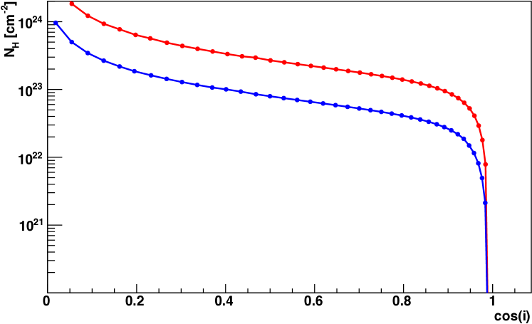
Figure 10: The column density as a function of the cosine of the inclination angle for the diverging biconical wind calculated for the system parameters of GX13+1. The blue line shows the predictions for a purely thermal wind, while the red includes a very simple treatment of radiation pressure. The source has $L/L_{\mathrm{Edd}}\sim 0.5$, so the thermal wind can be launched from closer in due to the lower effective gravity. This effect has a large impact on the predicted column, so the details of how this radiation pressure correction affects the velocity and density structure will be important in determining the line profiles.

We run MONACO on this wind structure to predict the detailed absorption line profiles for comparison to the 3rd order HEG data. Fig. 11 shows the result assuming an inclination angle of $80^{\circ}$ (Díaz Trigo et al., 2012) which gives the best fit to the data. This gives a fairly good match to the overall absorption, except for the highest velocity material seen in the data. Lower inclination angles give higher blueshift, but lower absorption line equivalent width, while higher inclination gives larger absorption line but lower blueshift (see Fig. 12). Thus it is not possible to completely reproduce the observed lines in GX13+1 with our simple radiation pressure corrected thermal wind model. This is not surprising, as radiation pressure will almost certainly change the velocity law by radiative acceleration as well as changing the launch radius. Full radiation hydrodynamic simulations are required to predict the resulting velocity and density structure. Nonetheless, our result demonstrates for the first time that hybrid thermal-radiative wind models can give a good overall match to the column and ionisation state of the wind in GX13+1, and that current data can already give constraints on the velocity and density structure of this material.

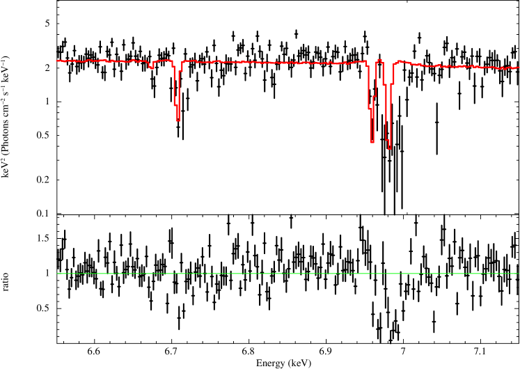
Figure 11: The model (red) and HEG 3rd order spectrum (black). The best fit inclination angle is $i=80^{\circ}$. This gives roughly the correct column of Fe XXV and XXVI at low velocity, but fails to match the observed higher velocity blue wing to the absorption features.

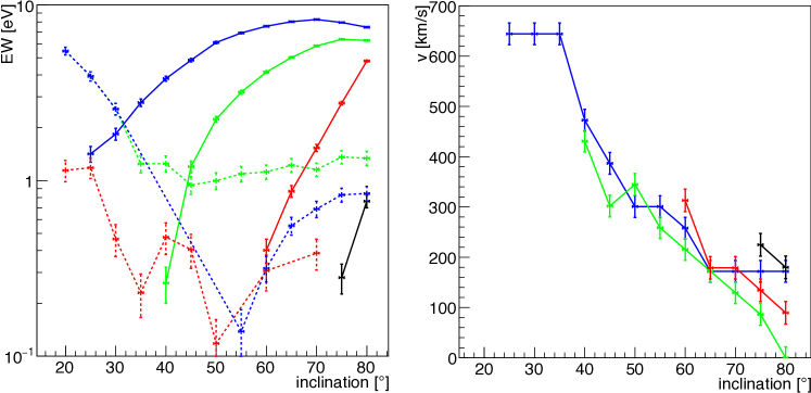
Figure 12: As in Fig. 8, but with the system parameters of GX 13+1 and the simplest radiation pressure correction to make a hybrid thermal/radiative wind.

6 Discussion and Summary

We construct a Monte-Carlo code to calculate detailed spectra from any given density and velocity distribution of highly ionised material. We use this to explore the absorption and emission lines of H and He-like Fe for the mass loss rates predicted from thermal wind models. We first use the radial streamline, constant velocity model of D18 which is able to reproduce the column derived from the hydrodynamic calculations of W96, but then extend this to a more realistic disc-wind geometry with gas accelerating along diverging streamlines, again reproducing the column from W96. The different assumed velocity and density structures for the thermal wind mass loss rates give different predictions for the overall ionisation state of the material, the resulting EW of emission and absorption lines, and their velocity shift. These show the potential of observations to test the detailed structure of the wind.

We apply the biconical disc wind model to some of the best data on winds from an LMXB. The neutron star GX13+1 shows strong and persistent absorption features in Chandra first order HETG spectra (Ueda et al., 2004; D’Aì et al., 2014), but here we show for the first time the higher resolution third order data. We find that while the source is fairly well matched to the parameters of the brightest fiducial simulation in terms of $T_{\mathrm{IC}}$, the higher luminosity ($L/L_{\mathrm{Edd}}=0.5$ compared to $0.3$ for the simulation) makes a significant impact on the predicted wind propertiesas it puts the source firmly into the regime where radiation pressure driving should become important.

We use the simple radiation pressure correction suggested by D18 and calculate the line profiles from a hybrid thermal-radiative wind. The additional radiation pressure driving means that the wind can be launched from much closer to the central source, and has higher mass loss rate. This is the first detailed test of the absorption line profiles predicted by physical wind models on any source other than the singular wind seen in GRO J1655-40 (Luketic et al., 2010). Our simulations quantitatively match many of the observed features except for the highest velocity material. This is not surprising, given the simplistic assumptions about the effect of radiation pressure. In future work we will use the wind velocity and density structure determined from full radiation hydrodynamics simulations in order to properly test the thermal-radiative wind models in GX13+1. Nonetheless, our current simulations already show that the thermal-radiative winds can potentially explain all of the wind absorption features seen in GX13+1, so that there is very little room for any additional magnetically driven winds in this source.

Appendix A The rotation velocity for radial streamlines

Here we give details of how we calculate the rotation velocity of each element of the wind for radial streamlines (Section 3). We have a linear radial grid, with 20 points from $R_{in}$ to $R_{out}$, so spaced by $dR=(R_{out}-R_{in})/20$. The inner shell has midpoint $R_{0}=R_{in}+dR/2$. We inject all the mass loss rate into this radial shell, distributed as $(1-\cos\theta)$, on a linear grid of 20 points in $\theta$. Each point on this inner shell is at a horizontal distance of $R_{0}\sin\theta$ from the black hole. We assume the material has the Keplarian velocity at this horizontal distance i.e. $v_{\phi}(R_{0},\theta)=\sqrt{GM/(R_{0}sin\theta)}$. Angular momentum conservation along each stream line (of constant $\theta$ for these radial streamlines) then gives $R_{0}\sin\theta v_{\phi}(R_{0},\theta)=R\sin\theta v_{\phi}(R,\theta)$ so $v_{\phi}(R,\theta)=(R/R_{0})v_{\phi}(R_{0},\theta)$

Appendix B Density and velocity structure for the diverging streamlines

The diverging wind streamlines originate from the focal point which is a distance $d$ below the black hole (see Fig 4). The innermost edge of the streamlines for the wind is at $\alpha_{min}=\arctan(R_{in}/d)$, and the outer edge is at $\alpha_{max}=\arctan(R_{out}/d)$. We make a linear grid so there are 40 angle elements in the wind, separated by $d\alpha=(\alpha_{max}-\alpha_{min})/40$ so that $\alpha_{i}=\alpha_{0}+id\alpha$ for $i=0\ldots 40$. We have $\alpha_{0}$ as a free parameter, set by comparison to the results of W96 (see section 4)

The maximum ’streamline’ length below the disc is from $\alpha_{max}$, where $D=\sqrt{d^{2}+R_{out}^{2}}$. We follow this for the same length above the disc. This defines the outer radius of the simulation box which is $R_{max}=2\sqrt{d^{2}+R_{out}^{2}}$. We take the inner edge at $R_{in}=0.1R_{IC}$.

We superpose a standard $\theta$ grid on this (measuring down from the z-axis to radial lines from the centre: Fig.13). We set $\theta_{0}$ to the point where the innermost streamline edge (at angle $\alpha_{0}$) reaches $R_{max}$ from the origin, and take 41 angles from this to $\pi/2$, giving $\theta_{j}(j=0,1..40)$. We make shells using the crossing points of these angles $\theta_{j}$ with the initial angles $\alpha_{i}$ (Fig.13). We also define the midpoint angles $A_{i}=(\alpha_{i}+\alpha_{i+1})/2$ and $\Theta_{j}=\frac{1}{2}(\theta_{j}+\theta_{j+1})$ .

The velocity along each stream line at a distance $l_{ij}$ from its launch point on the disc at radius $R_{i}=d\tan A_{i}$ is

$$v_{l}(R_{i},l_{ij})=f_{v}c_{ch}(R_{i})\sqrt{\frac{l_{ij}}{R_{i}}}$$ (B.1)

where

$$l_{ij}=D_{ij}-d/\cos A_{i},D_{ij}=d\frac{\sin\Theta_{j}}{\sin(\Theta_{j}-A_{i})}$$ (B.2)

for a characteristic sound speed $c_{ch}(R_{i})=\sqrt{\frac{kT_{ch}(R_{i})}{\mu m_{p}}}$ defined from the characteristic temperature

$$T_{ch}(R_{i})=\left(\frac{L}{L_{cr}}\right)^{2/3}(R_{i}/R_{IC})^{-2/3}$$ (B.3)

where the critical luminosity, $L_{cr}$ is

$$L_{cr}=\frac{1}{8}\left(\frac{m_{e}}{\mu m_{p}}\right)^{1/2}\left(\frac{m_{e}c^{2}}{kT_{IC}}\right)^{1/2}L_{Edd}$$ (B.4)

(see Done et al. 2018) and $f_{v}$ is free parameter which is determined by comparing with the results of W96.

We calculate the density of each shell $n_{ij}$ assuming mass conservation along each streamline.

$$n_{ij}=\frac{\Delta\dot{M}_{wind}(R_{i})}{m_{I}v_{l}(R_{i},l_{ij})4\pi D_{ij}^{2}(\cos\alpha_{i}-\cos\alpha_{i+1})}$$ (B.5)

where

$$\Delta\dot{M}_{wind}(R_{i})=2\pi\dot{m}(R_{i})R_{i}\Delta R_{i}\times 2=4\pi\dot{m}(R_{i})R_{i}d(\tan\alpha_{i+1}-\tan\alpha_{i})$$ (B.6)

The total mass loss rate at a given luminosity $L$ is $\dot{M}_{wind}=\sum_{i}\Delta\dot{M}_{wind}(R_{i})=2.0\times 10^{19}~{}\mathrm{g/s}~{}(L/L_{edd}=0.3),~{}8.0\times 10^{18}~{}\mathrm{g/s}~{}(L/L_{edd}=0.08),~{}2.1\times 10^{18}~{}\mathrm{g/s}~{}(L/L_{edd}=0.01)$.

Finally we, calculate the column density.

$$N_{H}(\Theta_{j})=\sum_{i}n_{ij}\Delta h_{ij}$$ (B.7)

where

$$\Delta h_{ij}=d(\frac{\sin\alpha_{i+1}}{\sin(\Theta_{j}-\alpha_{i+1})}-\frac{\sin\alpha_{i}}{\sin(\Theta_{j}-\alpha_{i})})$$ (B.8)

We assume Keplerian velocity on the disc plane ($\theta=\pi/2$ which is at $j=40$) so that

$$v_{\phi i,40}=\sqrt{\frac{GM}{D_{i,40}\sin A_{i}}}$$ (B.9)

and assume the angular momentum conversation along stream line so that

$$v_{\phi ij}=\frac{v_{\phi i,40}D_{i,40}\sin A_{i}}{D_{ij}\sin A_{i}}=\frac{v_{\phi i,40}D_{i,40}}{D_{ij}}$$ (B.10)

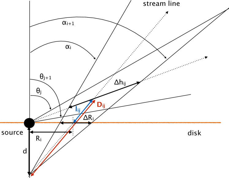
Figure 13: Details of the model geometry for the diverging wind streamlines.

References

- Agostinelli et al. (2003) Agostinelli S., et al., 2003, Nucl. Inst. Meth. Phys. Res. A, 506, 250
- Bandyopadhyay et al. (1999) Bandyopadhyay R. M., Shahbaz T., Charles P. A., Naylor T., 1999, MNRAS, 306, 417
- Begelman et al. (1983) Begelman M. C., McKee C. F., Shields G. A., 1983, ApJ, 271, 70
- Blandford & Payne (1982) Blandford R. D., Payne D. G., 1982, MNRAS, 199, 883
- Clarke & Alexander (2016) Clarke C. J., Alexander R. D., 2016, eprint arXiv:1605.04089, 3051, 3044
- Corbet et al. (2010) Corbet R. H. D., Pearlman A. B., Buxton M., Levine A. M., 2010, ApJ, 719, 979
- D’Aì et al. (2014) D’Aì A., Iaria R., Di Salvo T., Riggio A., Burderi L., Robba N. R., 2014, A&A, p. 13
- Díaz Trigo & Boirin (2016) Díaz Trigo M., Boirin L., 2016, Astronomische Nachrichten, 337, 368
- Díaz Trigo et al. (2012) Díaz Trigo M., Sidoli L., Boirin L., Parmar A., 2012, A&A, 543, A50
- Díaz Trigo et al. (2014) Díaz Trigo M., Migliari S., Guainazzi M., 2014, A&A, 76, 1
- Done et al. (2018) Done C., Tomaru R., Takahashi T., 2018, MNRAS, 473, 838
- Fukumura et al. (2014) Fukumura K., Tombesi F., Kazanas D., Shrader C., Behar E., Contopoulos I., 2014, ApJ, 780, 120
- Fukumura et al. (2017) Fukumura K., Kazanas D., Shrader C., Behar E., Tombesi F., Contopoulos I., 2017, Nature Astronomy, 1, 0062
- Hagino et al. (2015) Hagino K., Odaka H., Done C., Gandhi P., Watanabe S., Sako M., Takahashi T., 2015, MNRAS, 446, 663
- Hashizume et al. (2015) Hashizume K., Ohsuga K., Kawashima T., Tanaka M., 2015, PASJ, 67, 1
- Higginbottom & Proga (2015) Higginbottom N., Proga D., 2015, ApJ, 807, 107
- Kallman & Bautista (2001) Kallman T., Bautista M., 2001, ApJS, 133, 221
- Knigge et al. (1995) Knigge C., Woods J. A., Drew J. E., 1995, MNRAS, 273, 225
- Long & Knigge (2002) Long K. S., Knigge C., 2002, ApJ, 579, 725
- Luketic et al. (2010) Luketic S., Proga D., Kallman T. R., Raymond J. C., Miller J. M., 2010, ApJ, 719, 515
- Miller et al. (2006) Miller J. M., Raymond J., Fabian A., Steeghs D., Homan J., Reynolds C. S., van der Klis M., Wijnands R., 2006, Nature, 441, 953
- Miller et al. (2012) Miller J. M., et al., 2012, ApJ, 759, L6
- Miller et al. (2015) Miller J. M., Fabian A. C., Kaastra J., Kallman T., King A. L., Proga D., Raymond J., Reynolds C. S., 2015, ApJ, 814, 87
- Neilsen et al. (2016) Neilsen J., Rahoui F., Homan J., Buxton M., 2016, ApJ, 822, 20
- Odaka et al. (2011) Odaka H., Aharonian F., Watanabe S., Tanaka Y., Khangulyan D., Takahashi T., 2011, ApJ, 740, 103
- Odaka et al. (2016) Odaka H., Yoneda H., Takahashi T., Fabian A., 2016, MNRAS, 462, 2366
- Ponti et al. (2012) Ponti G., Fender R. P., Begelman M. C., Dunn R. J. H., Neilsen J., Coriat M., 2012, MNRAS: Letters, 422, 11
- Proga & Kallman (2002) Proga D., Kallman T. R., 2002, ApJ, 20, 455
- Shahbaz et al. (1998) Shahbaz T., Charles P. A., King A. R., 1998, MNRAS, 301, 382
- Shidatsu et al. (2016) Shidatsu M., Done C., Ueda Y., 2016, ApJ, 823, 159
- Sim et al. (2010) Sim S. a., Proga D., Miller L., Long K. S., Turner T. J., Reeves J. N., 2010, MNRAS, 408, 1369
- Ueda et al. (2004) Ueda Y., Murakami H., Yamaoka K., Dotani T., Ebisawa K., 2004, ApJ, 609, 325
- Watanabe et al. (2006) Watanabe S., et al., 2006, ApJ, 651, 421
- Waters & Proga (2012) Waters T. R., Proga D., 2012, MNRAS, 426, 2239
- Woods et al. (1996) Woods D. T., Klein R. I., Castor J. I., McKee C. F., Bell J. B., 1996, ApJ, 461, 767