Entropy Guided Spectrum Based Bug Localization Using Statistical Language Model

Abstract

Locating bugs is challenging but one of the most important activities in software development and maintenance phase because there are no certain rules to identify all types of bugs. Existing automatic bug localization tools use various heuristics based on test coverage, pre-determined buggy patterns, or textual similarity with bug report, to rank suspicious program elements. However, since these techniques rely on information from single source, they often suffer when the respective source information is inadequate. For instance, the popular spectrum based bug localization may not work well under poorly written test suite. In this paper, we propose a new approach, EnSpec, that guides spectrum based bug localization using code entropy, a metric that basically represents naturalness of code derived from a statistical language model. Our intuition is that since buggy code are high entropic, spectrum based bug localization with code entropy would be more robust in discriminating buggy lines vs. non-buggy lines. We realize our idea in a prototype, and performed an extensive evaluation on two popular publicly available benchmarks. Our results demonstrate that EnSpec outperforms a state-of-the-art spectrum based bug localization technique.

1 Introduction

Localizing bugs is an important, time consuming, and expensive process, especially for a system at-scale. Automatic bug localization can play an important role in saving developers’ time in debugging, and thus, may help developers fixing more bugs in a limited time. Using various statistical and program analysis approaches, these bug localization techniques automatically identify suspicious code elements that are highly likely to contain bugs. Developers then manually examine these suspicious code to pinpoint the bugs.

Existing bug localization techniques can be broadly classified into two categories: i) test coverage-based dynamic approaches [30, 2, 59, 14, 37, 38], and ii) pattern-based [15, 19, 18, 13] or information retrieval-based (IR) static approaches [44, 60, 48, 58]. Dynamic approaches first run all the test cases, and then analyze the program statements covered by passing and failing test cases. For example, spectrum based bug localization (${\cal S}{\cal B}{\cal B}{\cal L}$), a popular dynamic bug localization technique, prioritizes the program elements for debugging that are executed more by failing test cases than by passing test cases. In contrast, static approaches do not run any test cases. Rather, it searches for some previously known buggy patterns in source code or looks for buggy files based on bug reports.

Both of these bug localization approaches have their own set of advantages and disadvantages. For instance, static methods are often imprecise or inaccurate. On the other hand, the accuracy of dynamic approaches is highly dependent on the quality (code coverage, etc.) of the test suite. In real world projects, most of the test suite may not have enough code coverage to locate bugs efficiently. Therefore, in many cases, developers do not get the full benefit of bug localization techniques [29] and have to significantly rely on manual effort and prior experiences.

Besides static and dynamic properties of a program, it has also been observed that how developers write code is also important for code quality [25]. Real-world software that are developed by regular programmers tend to be highly repetitive and predictable [22]. Hindle et al.was the first to show that such repetitiveness can be successfully captured by a statistical language model [27]. They called this property as naturalness of code and measured it by standard information theory metric entropy. The less entropy a code snippet exhibits, the more the code is natural. Inspired by this phenomena, Ray et al. [45] investigated if there is any correlation between buggy code and entropy. They observed that buggy codes are in general less natural, i.e. they have higher entropy than non-buggy code.

In this paper, our key intuition is that, since the high entropic code tends to be buggy [45, 11, 54], code entropy can be an effective orthogonal source of information to ${\cal S}{\cal B}{\cal B}{\cal L}$ to improve the overall accuracy of bug localization. This notion seems to be plausible since from a set of suspicious code, as reported by a standard ${\cal S}{\cal B}{\cal B}{\cal L}$ technique, experienced programmers often intuitively identify the actual bugs because buggy code elements are usually a bit unnatural than rest of the corpus. If entropy can improve ${\cal S}{\cal B}{\cal B}{\cal L}$, it would be particularly useful when a test suite is not strong enough to discriminate buggy lines or when the suspicious scores of many lines are the same. Furthermore, to realize this hybrid approach, we only need source code (no other external meta-source), which is always available to the developers.

To this end, we introduce EnSpec, that automatically calculates the entropy for each program line and combines with a state-of-the-art ${\cal S}{\cal B}{\cal B}{\cal L}$ using a machine learning technique to return a ranked list of suspicious lines for investigation. Here, we studied bug localization at line granularity to ensure maximum benefit to the developers, although locating bugs in method and file-granularity is also possible. We performed an extensive evaluation of EnSpec on two popular publicly available bug-dataset: Defects4J [32] and ManyBugs [34] written in Java and C respectively. In total, we studied more than 500 bugs (3,715 buggy lines) bugs, around 4M LOC from 10 projects.

Overall, our findings corroborate our hypothesis that entropy can indeed improve bug localization capability of spectrum based bug localization technique. We further evaluate EnSpec for both C and Java projects showing that the tool is not programming language dependent. In particular, our results show that:

• Entropy score, as captured by statistical language models, can significantly improve bug localization capability of standard ${\cal S}{\cal B}{\cal B}{\cal L}$ technique.

• Entropy score also boosts ${\cal S}{\cal B}{\cal B}{\cal L}$ in cross-project bug localization settings.

In summary, we make the following contributions in this paper:

1. We introduce the notion of entropy in spectrum based bug localization.

2. We present EnSpec that effectively combine entropy score with the suspicious score of spectrum based bug localization using a machine learning technique.

3. We provide an extensive evaluation of EnSpec on two publicly available benchmarks that demonstrates the effectiveness of our approach.

2 Preliminaries

In this section, we discuss the preliminaries and backgrounds of our work.

2.1 Spectrum-based Bug Localization

Given a buggy code-base with at least one bug reproducing test case, a spectrum-based bug localization technique (${\cal S}{\cal B}{\cal B}{\cal L}$) ranks the code elements under investigation (e.g., files/classes, functions/methods, blocks, or statements) based on the execution traces of passing and failing test cases. Therefore, in this approach, first the subject program is instrumented at an appropriate granularity to collect the execution trace of each test case (test spectra). The basic intuition behind ${\cal S}{\cal B}{\cal B}{\cal L}$ is that the more a code element appears in failing traces (but not in passing traces), the more suspicious the element to be buggy.

Table 1: Spectrum based suspiciousness score of program element e

	#passed	#failed	spectrum
	test	test	score
total tests	$P$	$F$	$S=Func(e_{p},e_{f},n_{p},n_{f})$
e executed	$e_{p}$	$e_{f}$	$S_{Tarantula}=\frac{\frac{e_{f}}{F}}{\frac{e_{f}}{F}+\frac{e_{p}}{P}}$
e not executed	$n_{p}$=$P$-$e_{p}$	$n_{f}$=$F$-$e_{f}$	$S_{ochai}=\frac{e_{f}}{\sqrt{(e_{f}+e_{p})(e_{f}+n_{f})}}$

More specifically, for a given program element $e$, ${\cal S}{\cal B}{\cal B}{\cal L}$ records how many test cases execute and do not execute $e$, and computes the following four metrics: the number of (i) tests passed ($e_{p}$) and (ii) tests failed ($e_{f}$) that executed $e$, and the number of (iii) tests passed ($n_{p}$) and (iv) tests failed ($n_{f}$) that did not execute $e$. A suspiciousness score is calculated is calculated as a function of these four metric: $S=Func(e_{p},e_{f},n_{p},n_{f})$, as shown in Table 1. The table also presents two widely used suspiciousness score measure: Tarantula and Ochai. ${\cal S}{\cal B}{\cal B}{\cal L}$ ranks the program elements in a decreasing order of suspiciousness and presents to the developers for further investigation to fix the bug [57]. These scores also help to repair program automatically [35].

2.2 Language Models

Although real-world software programs are often large and complex, the program constructs (such as tokens) are repetitive, and thus provide useful predictable statistical property [26, 46, 51, 20]. These statistical properties of code resemble natural languages, and thus, natural language models can be leveraged for software engineering tasks.

Cache based N-gram Model ($gram): Hindle et al.introduced n-gram model for software code [27], which is essentially an extension of n-gram language model used in natural language processing tasks based on the Markov independence assumption [9]. If a sequence, $s$ consists of $m$ tokens ($a_{1}a_{2}a_{3}...a_{m}$), according to the Full Markov Model, the probability, $p(s)$, of that sequence is given in Equation 1

$$\small p(s)=p(a_{1})p(a_{2}|a_{1})p(a_{3}|a_{1}a_{2})...p(a_{m}|a_{1}a_{2}...a_{m-1})$$ (1)

N-gram model is a simplification of full Markov model based on the assumption that every token is dependent on previous $n-1$ token, where $n$ is a model parameter. Essentially with $n=\infty$, the model converges to the full Markov model. Since, actual probabilities are very difficult to find, researchers often use empirical probabilities to represent actual probabilities, which is highly dependent on the training data. Initially, the probability of a token or any n-gram which is not seen in the corpus will be zero resulting the total probability to be zero. To overcome this problem Hindle et al. [27] also adopted smoothing techniques from natural language processing literature.

Tu et al. [52] further improved the above model based on the observation that source code tends to be highly localized, i.e. particular token sequences may occur often within a single file or within particular classes or functions. They proposed a $gram model that introduces an additional cache—list of n-grams curated from local context and used them in addition to a global n-gram model. They also defined the entropy of a code sequence $S$ by language model $M$ by Equation 2:

$$\small H_{M}(S)=-\frac{1}{N}\log_{2}p_{M}(S)=-\frac{1}{N}\sum\limits_{i=1}^{N}\log_{2}P(t_{i}|h)$$ (2)

Language model to predict buggy code: Ray et al. [45] demonstrated that there is a strong negative correlation between code being buggy and the naturalness of code. When a simple $gram model is trained on previous versions of project source code and applied to calculate naturalness of code snippet, buggy codes are shown to exhibit higher unnaturalness than the non-buggy codes. They introduced a syntax-sensitive entropy model to measure naturalness of code. In their investigation, they found that some token types such as packages, methods, variable names are less frequent, and hence high entropic than others. They normalized the entropy score and derived a Z-score with line-type information from the program’s Abstract Syntax Tree (AST). The Z-score is defined as:

$$\small\$gram+type=\frac{entropy_{line}-\mu_{type}}{SD_{type}}$$ (3)

In Equation 3, $\mu_{type}$ is the mean $gram model entropy of a given line type, and $SD_{type}$ is the standard deviation of that line type. This Z-score gives the syntax-sensitive entropy. They reported that, buggy lines of codes are usually unnatural and highly entropic. With further investigation, they also found that, when developers fixed those buggy lines of codes, the entropy of the code decreased. In this work, we used state of the art $gram model along with syntax-sensitive entropy model.

3 Motivating Example

In this section, we present a real-world example that motivated us to incorporate the naturalness property of code (i.e. entropy based features) in ${\cal S}{\cal B}{\cal B}{\cal L}$ to overcome a key limitation of ${\cal S}{\cal B}{\cal B}{\cal L}$.

The main limitation of testing based bug localization approaches, such as ${\cal S}{\cal B}{\cal B}{\cal L}$, is that the quality of their results highly depend on the quality of test cases. If the passing test cases have low code coverage, an ${\cal S}{\cal B}{\cal B}{\cal L}$ tool may return a large number of program elements with high suspiciousness score, most of which are false positives. However, generating an adequate test suite is incredibly difficult. Therefore, in many cases ${\cal S}{\cal B}{\cal B}{\cal L}$ performs poorly.

--- /Closure/89/buggy/src/com/google/javascript/jscomp/ GlobalNamespace.java

+++ /Closure/89/fix/src/com/google/javascript/jscomp/ GlobalNamespace.java ⬇ - if (type != Type.FUNCTION && aliasingGets > 0) { //Entropy before patch 7.36 + if (aliasingGets > 0) { //Entropy after patch 1.15 return false; }

Table 2: Effectiveness of entropy based features to improve ${\cal S}{\cal B}{\cal B}{\cal L}$

Table 2 presents a patch that fixed a bug in Closure compiler (Defects4J bug ID: 89). The buggy line, marked in red, was never used in the existing corpus before. Hence, the line was unnatural to a ${\cal L}{\cal M}$ with a high entropy score of $7.36$. When developer fixed the bug (see green line), the code becomes more natural with a reduced entropy score of $1.15$. A traditional state-of-the art ${\cal S}{\cal B}{\cal B}{\cal L}$ technique placed the buggy line at 57^th position, while EnSpec using both entropy and spectrum based features, placed the line at 12^th position in the ranked list of suspicious lines. This shows that entropy of code, as derived from ${\cal L}{\cal M}$, can play an important role to improve the ranking of the actual buggy lines.

4 Proposed Approach

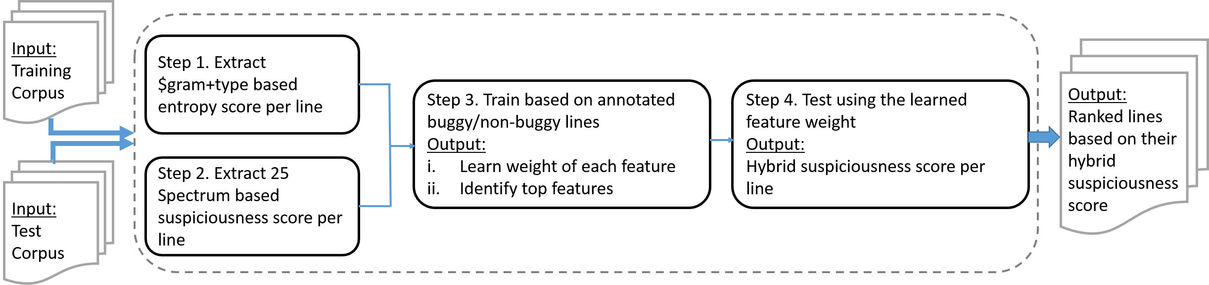
Figure 1: EnSpec Workflow

In this section, we describe our tool, EnSpec. An overview of our approach is shown in Figure 1. The goal of EnSpec is to localize bugs using a hybrid bug localization technique: a combination of dynamic spectrum based bug localization (${\cal S}{\cal B}{\cal B}{\cal L}$) and static natural language model based defect prediction (${\cal L}{\cal M}$). EnSpec takes two sets of code corpus as input—training and testing set. Next, EnSpec works in following four steps: Step-1. EnSpec collects entropy score per code element based on a language model for each input project. Step-2. For each project version in the training and test corpus, EnSpec records test coverage and collects various ${\cal S}{\cal B}{\cal B}{\cal L}$ based suspiciousness scores per code element. Step-3. In this step, EnSpec learns from the training data, how the suspiciousness scores and entropy collected in above two steps relate to buggy/non-buggy classes and learns feature weight. In Section 5.2, we describe the data collection phase in more detail: how we annotate each code element as buggy/non-buggy. Step-4. Based on the learned feature-weight, EnSpec assigns a suspiciousness score of each code element in the test corpus. The suspiciousness score depicts the probability of a code element to be buggy. Finally, the output of EnSpec is a ranked list of code elements based on their decreasing suspiciousness score.

In theory, EnSpec should work on code elements at any granularity—line, method, file, etc. In this paper, we use EnSpec to localize bugs at a line granularity. In the following section, we describe these steps in details.

Step-1: Generating entropy using ${\cal L}{\cal M}$

For generating entropy per program line, we adopted the $gram language model proposed by Tu et al. [52]. For every line in source code we calculated following three entropy values:

1. Forward Entropy $(E_{f})$: Entropy value of a token is calculated based on the probability of seeing the token given its prefix token sequences. We calculate this entropy by parsing the file from beginning to end, i.e. considering the token sequences as it is in the source file.

2. Backward Entropy $(E_{b})$: Entropy value of a token is calculated based on the probability of seeing the token given its suffix token sequences. We calculate this entropy by parsing the file in reverse order, i.e. from end to beginning.

3. Average Entropy $(E_{a})$: This entropy value is calculated as the average of $E_{f}$ and $E_{b}$.

We use these three values as our ${\cal L}{\cal M}$ based features. We further normalized these values based on their AST type, as shown in Equation 3. We refer these three normalized entropy values as entropy related features in the rest of the paper.

Table 3: 25 suspiciousness scores from literature that are used as ${\cal S}{\cal B}{\cal B}{\cal L}$ features in EnSpec

Metric	Formula	Metric	Formula	Metric	Formula	Metric	Formula
Tarantula	$\frac{\frac{e_{f}}{e_{f}+n_{f}}}{\frac{e_{f}}{e_{f}+n_{f}}+\frac{e_{p}}{e_{p}+n_{p}}}$	Ochiai	$\frac{e_{f}}{\sqrt{(e_{f}+e_{p})(e_{f}+n_{f})}}$	Jaccard	$\frac{e_{f}}{e_{f}+e_{p}+n_{f}}$	SimpleMatching	$\frac{e_{f}+n_{p}}{e_{f}+e_{p}+n_{f}+n_{p}}$
S$\phi$rcenDice	$\frac{2e_{f}}{2e_{f}+e_{p}+n_{f}}$	Kulczynskil	$\frac{e_{f}}{e_{p}+n_{f}}$	RusselRao	$\frac{e_{f}}{e_{f}+e_{p}+n_{f}+n_{p}}$	RogersTanimoto	$\frac{e_{f}+n_{p}}{e_{f}+e_{p}+2n_{f}+e_{P}}$
M1	$\frac{e_{f}+n_{p}}{e_{p}+n_{f}}$	M2	$\frac{e_{f}}{e_{f}+n_{p}+2e_{p}+2e_{f}}$	Overlap	$\frac{e_{f}}{min(e_{f},e_{p},n_{f})}$	Ochiai2	$\frac{e_{f}n_{p}}{\sqrt{(e_{f}+e_{p})(n_{f}+n_{p})(e_{f}+n_{p})(e_{p}+n_{f})}}$
Dice	$\frac{2e_{f}}{e_{f}+e_{p}+n_{f}}$	Ample	$\left|\frac{e_{f}}{e_{f}+n_{f}}-\frac{e_{p}}{e_{p}+n_{p}}\right|$	Hamann	$\frac{e_{f}+n_{p}-e_{p}-n_{f}}{e_{f}+e_{p}+n_{f}+n_{p}}$	Zoltar	$\frac{e_{f}}{e_{f}+e_{p}+n_{f}+\frac{10000n_{f}e_{p}}{e_{f}}}$
Goodman	$\frac{2e_{f}-n_{f}-e_{p}}{2e_{f}+n_{f}+e_{p}}$	Sokal	$\frac{2e_{f}+2e_{p}}{2e_{f}+2e_{p}+n_{f}+n_{p}}$	Hamming	$e_{f}+n_{p}$	Kulczynski2	$\frac{1}{2}\left(\frac{e_{f}}{e_{f}+n_{f}}+\frac{e_{f}}{e_{f}+n_{p}}\right)$
Euclid	$\sqrt{e_{f}+n_{p}}$	Anderberg	$\frac{e_{f}}{e_{f}+2e_{p}+2n_{f}}$	Wong1	$e_{f}$	Wong2	$e_{f}-e_{p}$
Wong3	$e_{f}-h,\leavevmode\nobreak\ where\leavevmode\nobreak\ h=\left\{\begin{array}[]{ll}e_{p}&\text{if}\leavevmode\nobreak\ e_{p}\leq 2\\ 2+0.1(e_{p}-2)&\text{if}\leavevmode\nobreak\ 2\leq e_{p}\leq 10\\ 2.8+0.01(e_{p}-10)&\text{if}\leavevmode\nobreak\ e_{p}\geq 10\\ \end{array}\right.$

Step-2: Extracting suspiciousness score using ${\cal S}{\cal B}{\cal B}{\cal L}$ techniques.

For all the input project versions, we first instrument the source code to record program execution traces, or coverage data. Both Defects4J and ManyBugs dataset provide APIs for collecting such coverage data. Then, to collect the execution traces, we extract the test classes and test methods from the project source code and run the test cases. We record the execution traces for each test case with its passing/failing status. These test spectra characterize the program’s behavior across executions by summarizing how frequently each source code line was executed for passing and failing tests. Now for each line we calculate 4 values $(e_{p},e_{f},n_{p},n_{f})$, as described in Section 2. Next, using these 4 values, we generate 25 suspiciousness scores, as described by Xuan et al. [57]. We use these 25 scores(see Table 3) as our ${\cal S}{\cal B}{\cal B}{\cal L}$ features.

The next two steps implement the training and testing phase of a classifier based on buggy and non-buggy program lines. We adapted Li et al.’s learning to rank algorithm for this purpose [36].

Step-3: Training Phase

Given a set of buggy and non-buggy lines, EnSpec learns the relation between ${\cal S}{\cal B}{\cal B}{\cal L}$ and entropy related features on the bugginess of program lines.

First, all lines in the training dataset were annotated with a relevance score of bugginess: $R_{b}$ for each buggy line, and $R_{g}$ for each non-buggy line, where $R_{b}>R_{g}$. Thus, each line $l$ in the training code corpus is represented as a tuple, $\langle Sp_{l},En_{l},R_{l}\rangle$, where $Sp_{l}$ is a set of ${\cal S}{\cal B}{\cal B}{\cal L}$ features, $En_{l}$ is a set of entropy related features, and $R_{l}\in\{R_{b},R_{g}\}$ is the bug-relevance score. Then, we pass the whole corpus to a machine learner, which learns the probability distribution $P(R_{l}|Sp_{l},En_{l})$ of the relevance scores given the feature values.

Step-4: Testing Phase

In testing phase, for each line $l$ in the test corpus, we compute a suspiciousness score ($susp$) based on equation  4.

$$\begin{split}susp_{l}=f(R_{b})&*P(R_{b}|Sp_{l},En_{l})\\ &+f(R_{g})*P(R_{b}|Sp_{l},En_{l})\end{split}$$ (4)

Here, $f(R_{b})$ and $f(R_{g})$ are monotonically increasing functions. To keep things simple, we used identity function, i.e., $f(R_{b})=R_{b}$ and $f(R_{g})=R_{g}$, which is monotonic as well. This transforms equation  4 into:

$$\begin{split}susp_{l}&=\sum_{R_{l}\in\{R_{b},R_{g}\}}{R_{l}*P(R_{l}|Sp_{l},En_{l})}\\ &=\mathbb{E}[R_{l}|Sp_{l},En_{l}]\end{split}$$ (5)

We use ensemble [17] of $M$ different models trained on randomly sampled subset of original dataset. Each model $M_{k}$ computes a suspiciousness score $susp_{l}^{k}$, based on the expected relevance score of equation 5. Our final hybrid suspiciousness score is calculated by equation 6:

$$HySusp_{l}=\frac{1}{M}\sum_{k=1}^{M}{susp_{l}^{k}}$$ (6)

EnSpec outputs a ranked list of source code lines based on the decreasing order of hybrid suspiciousness score (HySusp), line with highest suspiciousness tops the list.

5 Experimental Setup

In this section, we describe how we setup our experiment to evaluate EnSpec. In particular, we describe the subject systems, how we collect data, evaluation metric, and research questions to evaluate EnSpec.

Table 4: Study Subjects

Dataset	Project	KLoc	#Tests	#Bugs	#Buggy Lines	#Buggy Lines
					(original dataset)	(original + evolutionary)
	JFreechart	96	2,205	26	22	32
	Closure compiler	90	7,927	133	64	586
Defects4J [32]	Apache commons-math	85	3,602	106	38	816
(Language: Java)	Joda-Time	28	4,130	27	46	97
	Apache commons-lang	22	2,245	65	50	230
	Total	321	20,109	357	220	1761
	Libtiff	77	78	24	944	-
	Lighttpd	62	295	9	26	-
ManyBugs [34]	Php	1,099	8,471	104	503	-
(Language: C)	Python	407	355	15	93	-
	Wireshark	2,814	63	8	388	-
	Total	4,459	9,262	160	1954	-

5.1 Study Subject

We used two publicly available bug dataset: Defects4J [32] and ManyBugs [34] (see Table 4). Defects4J dataset contains $5$ open source projects with $321$K lines of code, $357$ reproducible bugs, and $20$K total number of tests. All the Defects4J projects are written in Java. We also studied $5$ projects from ManyBugs benchmark dataset [34]. These are medium to large open source C projects, with total $4459$K lines of code, $160$ reproducible bugs, and $9262$ total test cases. In both datasets, each bug is associated with a buggy and its corresponding fix program versions. There are some failing test cases that reproduce the bugs in the buggy versions, while after the fixes all the test cases pass. The dataset also provides APIs for instrumentation and recording program execution traces.

5.2 Data Collection

Here we describe how we identified the buggy program statements. We followed two techniques as described below:

I. Buggy lines retrieved from original dataset. We compared each buggy program version with its corresponding fixed version; the lines that are deleted or modified in the buggy version are annotated as buggy program statements. To get the differences between two program versions, we used Defects4J APIs for Defects4J dataset. For every snapshot, ManyBugs dataset provides diff of different files changed during the fix revision. We directly used those diff files.

We notice that some bugs are caused due to the error of omission—tests fail due to missing features/functionalities in the buggy version. Fixing these bugs do not require deleting or modifying program statements in the buggy version, but adding new lines in the fixed version. In such cases, we cannot trivially annotate any of the existing lines in the buggy version as ‘buggy.’ We filter out such bugs from further consideration, as our goal in this work to locate existing buggy lines, as opposed to detecting error of omission. Table 4 shows the total number of buggy lines per project in the original dataset.

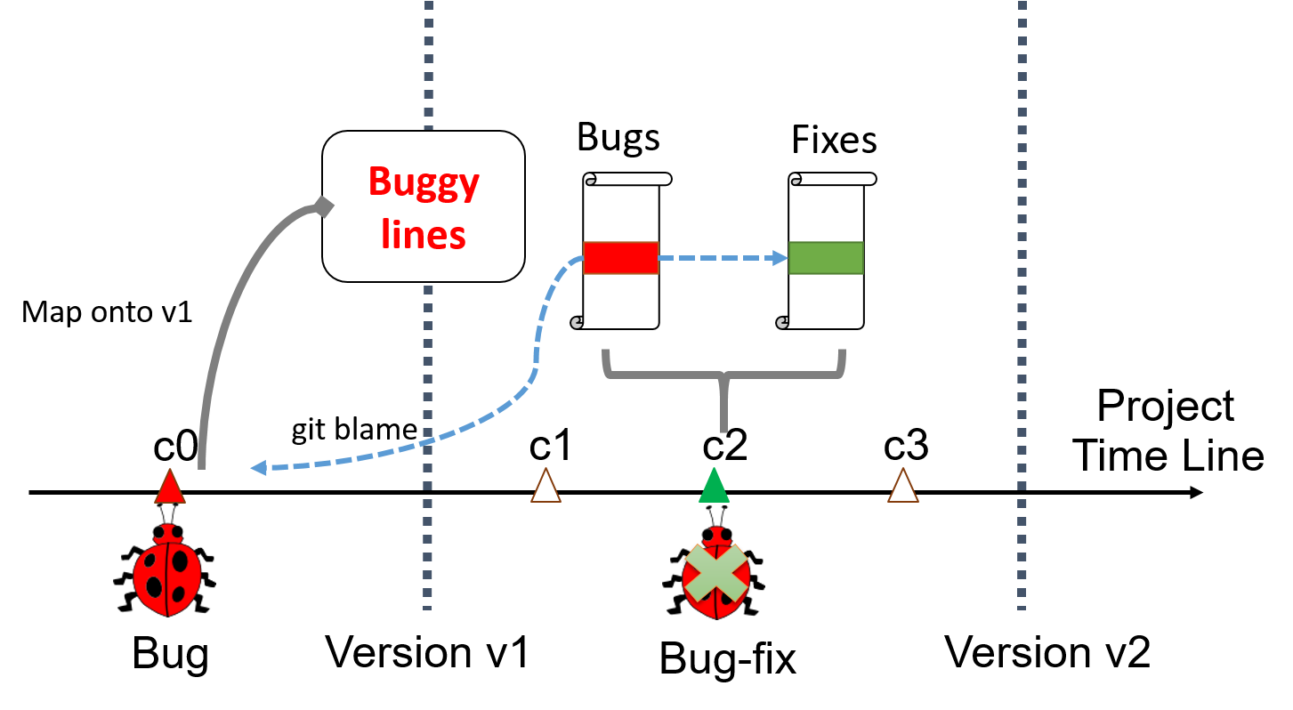
Figure 2: Evolutionary bug data retrieval: vertical dashed lines correspond to buggy project versions under investigation, each triangle represents project commit (c0$\ldots$c3). For every bug-fix commit (e.g., c2), as identified by keyword search, we first git-blame the buggy lines to identify the original bug-introducing commit (e.g., c0) and then map them to the corresponding project versions.(Adopted from Ray et al. [45])

II. Buggy lines retrieved from project evolution. As shown in Table 4, the percentage of buggy lines w.r.t. the total lines of code in Defects4J dataset is very small (0.07%). Such unbalanced data of buggy vs. non-buggy lines poses a threat to the efficiency of any classification probelm [28, 12]. To reduce such imbalance and thus increase the effectiveness of ${\cal S}{\cal B}{\cal B}{\cal L}$, previous work injects artificial bugs in the software system under tests [24, 49]. However, since the motivation of this research comes from the findings that bugs are unnatural [45], artificially introducing bugs like our predecessors may question our conclusions. To overcome this problem, we injected bugs that developers introduced in the source code in reality—we collected such bugs from project evolutionary history.

We adopted the similar strategy described in Ray et al. [45]. First, we identified bug-fix commits by searching a project’s commit logs using bug-fix related keywords: ‘error’, ‘bug’, ‘fix’, ‘issue’, ‘mistake’, ‘flaw’, and ‘defect’, following the methodology described by Mockus et al. [41]. Lines modified or deleted on those big-fix commits are marked as buggy. Then we identified the original commits that introduce these bugs using SZZ algorithm [50]. Next, we used git blame with --reverse option to locate those buggy lines in the buggy program version under investigation. Figure 2 illustrates this process.

Using this method, we found $1541$ additional buggy lines across all the versions of five Defects4J projects. Thus, in total, in this dataset, we studied $1761$ buggy lines, as shown in 4.

5.3 Evaluation Metric

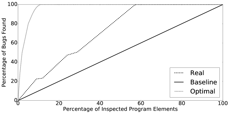
Figure 3: Example Cost Effectiveness (CE) curve for bug localization. Baseline shows CE while inspecting random program elements. At optimal CE, 100% of bugs are found when all the buggy program elemnets are inspected first. A real CE falls somewhere in between baseline and optimal.

To evaluate the bug localization capability of EnSpec, we adopted commonly used non-parametric measure from literature: Cost Effectiveness (CE) metric originally proposed by Arisholm et al. [4] to investigate defects in telecom softwares. The main assumption behind this metric is, cost behind bug localization is the inspection effort—the number of Program Element (PE) needs to be inspected before locating the bug, and the payoff is the percentage of bugs found. A Cost-Effectiveness(CE) curve shows percentage of inspected PE in x-axis and percentage of bugs found in y-axis.

If bugs are uniformly distributed in the source code, by randomly inspecting $n\%$ of source PE, one might expect to find $n\%$ bugs. The corresponding CE curve will be a straight line with $slope\leavevmode\nobreak\ \text{=}\leavevmode\nobreak\ 1$ (see Figure 3). This is our baseline. Any ranking metric assigns suspiciousness score to each PE for bug localization. Then, PEs are inspected based on the decreasing order of suspiciousness score. An optimal ranking metric would assign scores in a way that all buggy PEs are ranked prior to the non-buggy PEs. So, inspecting top PEs would cover 100% of the bugs. For any real bug localization techniques, e.g., Tarantula [30], Multric [57] etc., CE curve falls in between baseline and optimal.

AUCEC, the area of under the CE curve is a quantitative measurement describing how good a model is to find the bugs. Baseline AUCEC (random AUCEC) is 0.5. Optimal AUCEC would be very close to 1.00. This AUCEC metric is a non-parametric metric similar to the ROC curve and does not depend on bug distribution [45], thus becomes standard in bug-localization literature [16]. Higher AUCEC signifies higher prioritization of buggy lines over non-buggy lines and hence a better model. For example, for the optimal CE, 100% source program elements should not have to be inspected to find all the bugs; thus, optimal exhibits higher AUCEC than the baseline (see Figure 3). This intuition is the basis of our evaluation metric.

5.4 Implementation of EnSpec

We implemented EnSpec’s learning to rank technique as described in Step 3 & 4 of Section 4 using two approaches. First, we used RankBoost [21] algorithm. RankBoost algorithm uses boosting ensemble technique to learn model parameter for ranking training instances. At each iteration, it learns one weak ranker and then re-weights the training data. At the final stage, it combines all the weak rankers to assign scores to the test data. This algorithm is used in the past by Xuan et al. [57] for implementing ${\cal S}{\cal B}{\cal B}{\cal L}$ at method level bug localization. Though there are many competitive approaches to implement ${\cal S}{\cal B}{\cal B}{\cal L}$, Xuan et al.report the best results till date. Thus, we adapted their approach in EnSpec to locate bugs at line granularity. We used RankBoost implementation of standard RankLib [1] library for this purpose. There are two configurable parameters: $\beta$ (initial ranking metric) and $\gamma$ (number of neighbor). Following Xuan et al., we set these two parameter values to Tarantula and 10 respectively. Table 5 shows the result.

In the second approach, we used Random Forest Algorithm (RF) to implement the proposed learning to rank technique. Random Forest is an ensemble learning technique developed by Breiman [8] based on a combination of a large set of decision trees. Each tree is trained by selecting a random set of features from a random data sample selected from the training corpus. In our case, the algorithm, therefore, chooses some ${\cal S}{\cal B}{\cal B}{\cal L}$ and/or entropy related features randomly in training phase (step 3). RF then learns conditional probability distribution of the chosen features w.r.t. the bugginess of each line in the training dataset. In addition, RF learns the importances for different features for discrimination. During training, the model learns $M$ decision trees and corresponding probability distribution. In the testing phase, suspiciousness scores from each of the learned model, and calculate final suspiciousness score based on equation 6. For implementation, we used standard python scikit-learn package [10].

Table 5: Performance (AUCEC₁₀₀) comparison of two learning to rank implementations that are used to realize EnSpec. Only ${\cal S}{\cal B}{\cal B}{\cal L}$ related features are used to establish a baseline.

Project	RankBoost	Random Forest
JFreechart	0.847	0.908
Closure compiler	0.797	0.894
Apache commons-lang	0.824	0.862
Apache commons-math	0.864	0.876
Joda-Time	0.846	0.918
Libtiff	0.847	0.887
Lighttpd	0.753	0.806
Php	0.835	0.899
Python	0.788	0.807
Wireshark	0.864	0.829

We compare the performance of the above two approaches using AUCEC₁₀₀ score. For the comparison purpose, we only used ${\cal S}{\cal B}{\cal B}{\cal L}$ related features (i.e. did not include entropy scores), since we first wanted to measure how the two approaches perform in traditional ${\cal S}{\cal B}{\cal B}{\cal L}$ setting. Table 5 reports the result. For all of the studied projects, except Wireshark, Random Forest is performing better. Thus, we carried out rest of our experiments using Random Forest based implementation, since this gives the best ${\cal S}{\cal B}{\cal B}{\cal L}$ performance at line level, even when we compare against state of the art Xuan et al.’s technique.

5.5 Research Questions

To evaluate EnSpec, we investigate whether a good language model (${\cal L}{\cal M}$) that captures naturalness (hence unnaturalness) of a code element can improve spectrum based testing. Previously, Ray et al. [45] and Wang et al. [54] demonstrated that unnaturalness of code elements (measured in terms of entropy) correlate with bugginess. Thus, ${\cal L}{\cal M}$ can help in bug localization in a static setting. In contrast, ${\cal S}{\cal B}{\cal B}{\cal L}$ is a dynamic approach that relies on the fact that code elements that are covered by more negative test cases are more bug-prone. Therefore, to understand the effectiveness of EnSpec, we will investigate whether the combination of the two can improve bug-localization as a whole.

Since ${\cal L}{\cal M}$ based bug-localization approach says that more entropic code is more bug prone, and ${\cal S}{\cal B}{\cal B}{\cal L}$ says that code element covered by more negative test cases are more prone to bugs, to make the combined approach work, the difference between entropies of the buggy and non-buggy lines should be significant for the negative test spectra. Thus, to understand the potential of entropy, we start our investigation with the following research question:

RQ1. How is entropy associated with bugginess for different types of test spectra?

If the answer to the above question is affirmative for failing test spectra, entropy can be used along with ${\cal S}{\cal B}{\cal B}{\cal L}$ for bug-prediction. For every code element, ${\cal S}{\cal B}{\cal B}{\cal L}$ provides suspiciousness scores, and ${\cal L}{\cal M}$ predicts its uncertainty in terms of entropy. Thus, one may expect that among the lines with higher suspiciousness score, more entropic lines are even more likely to be buggy. We, therefore, investigate whether entropy can help improving the bug prediction capability of EnSpec over ${\cal S}{\cal B}{\cal B}{\cal L}$.

RQ2. Can entropy improve ${\cal S}{\cal B}{\cal B}{\cal L}$’s bug-localization capability?

To build a good ${\cal L}{\cal M}$ based bug localization technique, we need a large code corpus with adequate bug history; this is often challenging for smaller projects. A similar problem arises for history based defect prediction models—for newer projects enough history is usually not available to build a good model. In such case, researchers, in general, rely on the evolutionary history of other projects [62]. To mitigate the threat of using our proposed approach for smaller code base, we leverage such cross-project defect prediction strategy. We investigate, whether a language model trained on different projects can still improve ${\cal S}{\cal B}{\cal B}{\cal L}$’s performance.

RQ3. What is the effect of entropy on ${\cal S}{\cal B}{\cal B}{\cal L}$’s bug localization capability in a cross-project setting?

6 Result

In this section, we answer the research questions introduced in 5.5. Our investigation starts with whether the buggy lines in failing test spectrum are more entropic than non-buggy lines. Note that, all the buggy and non-buggy lines are annotated using the strategy described in 5.2.

RQ1. How is entropy associated with bugginess for different types of test spectra?

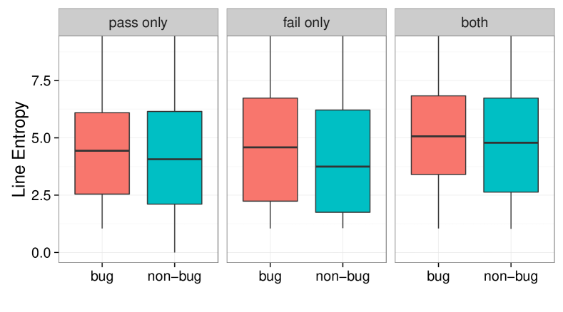
Type of	Percentage	Buggy Entropy > Non-buggy Entropy
test	buggy	Difference		Effect Size
spectra	lines	(95% conf interval)	p-value	(Cohen’s D)
Fail only	4.22	0.06 to 0.99	0.027	0.20 ( small )
Pass only	0.85	0.00 to 0.28	0.051	0.06 ( negligible )
Both	1.60	0.09 to 0.38	0.002	0.09 ( negligible )

Figure 4: For failing test spectra, buggy lines are more entropic than non-buggy lines; t-test confirms that the difference is statistically significant (p-value $<$ 0.05) with small Cohen’s D effect size. However, for other two spectra, the difference is negligible.

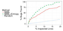
(a) Bug localization performance with an inspection budget of 20% of total lines

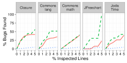
(b) Bug localization performance with an inspection budget of 5% of total lines for Defects4J dataset

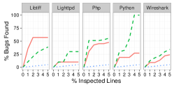
(c) Bug localization performance with an inspection budget of 5% of total lines for ManyBugs dataset

Project	AUCEC100	AUCEC100	Gain	Top Three Features
	(${\cal S}{\cal B}{\cal B}{\cal L}$)	(${\cal S}{\cal B}{\cal B}{\cal L}$ +Entropy)	(%)	Feature 1	Feature 2	Feature 3
JFreechart	0.908	0.956	5.305	Average Entropy	Ochiai	RogersTanimoto
Closure compiler	0.894	0.916	2.451	Average Entropy	Euclid	SimpleMatching
Apache commons-lang	0.862	0.943	9.368	Average Entropy	SimpleMatching	RogersTanimoto
Apache commons-math	0.876	0.883	0.708	Average Entropy	Jaccard	RogersTanimoto
Joda-Time	0.918	0.930	1.318	Average Entropy	Euclid	Hamming
Libtiff	0.887	0.904	2.004	Average Entropy	SimpleMatching	Hamming
Lighttpd	0.806	0.943	17.016	Average Entropy	Jaccard	Ochiai
Php	0.899	0.941	4.675	Average Entropy	Hamming	Euclid
Python	0.807	0.961	19.133	Average Entropy	Sokal	SimpleMatching
Wireshark	0.829	0.864	4.193	Average Entropy	Wong3	Ample
Average	0.869	0.924	6.617

Figure 5: Overall performance of EnSpec (${\cal S}{\cal B}{\cal B}{\cal L}$ + Entropy) vs. ${\cal S}{\cal B}{\cal B}{\cal L}$ for localizing buggy lines.

To answer this question, first, for each buggy version of Defects4J and ManyBugs dataset, we calculated the $gram entropy value for every line in the project’s source code. We also instrumented the source code to record the execution trace information at line level for passing and failing test cases. For Defects4J projects, we instrumented each file. Therefore, we recorded the execution traces for all files. However, ManyBugs projects were large in size (see 4); hence due to technical limitations, we only instrumented the buggy files for this data set. Note that, this is not an unreasonable assumption; one can use other human-based or automated techniques, e.g., statistical or information retrieval based defect prediction, to locate potential buggy files [43, 53, 48]. Additionally, many of our buggy files have hundreds of lines of code, which is similar to the size of the code tested in previous ${\cal S}{\cal B}{\cal B}{\cal L}$ analyses [31].

Next, we group the program lines based on the test execution traces: i) Fail Only: lines covered by only failing test cases (no passing test case exercise these lines), ii) Pass Only: lines covered by only passing test cases (no failing test cases exercised these lines), and iii) Both: lines covered by both failing and passing test cases. Note that, there is still a considerable number of program lines that are not covered by any test cases because the code coverage is not 100% for any of the studied test suite. Such non-executed program lines are out of scope for this research question. For each group, we studied the $gram entropy differences between buggy and non-buggy program lines. Figure 4 shows the result.

Buggy lines, in general, have higher entropy than non-buggy lines in all three groups, as shown in the boxplot. However, a t-test [61] (see the Table below of 4) confirms that for Fail Only spectra, the difference is statistically significant (p-value < 0.05), with a small Cohen’s D effect size. Note that, a similar effect size for overall buggy vs. non-buggy entropy was also reported by previous studies [45]. For Pass Only spectra, the difference is not statistically significant between buggy and non-buggy lines. Furthermore, although a small difference exists for Both spectra, the Cohen’s D effect size is negligible. These results are also confirmed by Wilcoxon non-parametric test [40, 61].

In summary, we conclude that entropy is associated with bugginess for lines covered by failing test cases, while for the lines not covered by the failing test cases, entropy does not show significant association. This could be due to many factors such as the complexity or nuance of bugs that are not captured adequately by the test cases, or simply because of the quality of the test suite if it does not exercise many non-buggy lines which is low entropic. Certainly, more research is needed. Nevertheless, this result is significant for our study. Since, in failing spectra, entropy can further discriminate buggy and non-buggy lines, entropy score on top of the ${\cal S}{\cal B}{\cal B}{\cal L}$ based suspiciousness score would enhance the bug localization capability. Additionally, since entropy does not differentiate between buggy and non-buggy lines in the passing spectra, it will not boost ${\cal S}{\cal B}{\cal B}{\cal L}$ suspiciousness score for them. Thus, we believe overall entropy would play an key role to improve ${\cal S}{\cal B}{\cal B}{\cal L}$ based bug localization by increasing the suspiciousness scores of the buggy lines that cause tests to fail.

Result 5.5: For failing test spectra, buggy lines, on average, are high entropic, i.e. less probable, than non-buggy lines.

So far, we have seen that entropy is associated with the bugginess of the code elements covered by failing test cases. Now, let us investigate whether EnSpec can leverage this property to localize bugs more effectively.

RQ2. Can entropy improve ${\cal S}{\cal B}{\cal B}{\cal L}$’s bug-localization capability?

To investigate this research question, we trained EnSpec’s model in two settings: i. ${\cal S}{\cal B}{\cal B}{\cal L}$ only: 25 different ${\cal S}{\cal B}{\cal B}{\cal L}$ based suspiciousness scores, as shown in Table 3 as features, and ii. ${\cal S}{\cal B}{\cal B}{\cal L}$ + Entropy: 25 different ${\cal S}{\cal B}{\cal B}{\cal L}$ based suspiciousness scores along with entropy related scores (see Section 4) as features, where entropies are generated by $gram+type language model (see equation 3). We computed AUCEC at 100% inspection budget for both the settings, $AUCEC_{sp}$ and $AUCEC_{en}$ respectively. The experiment is run 30 times per project and the final result is the average of those 30 runs. To understand relative improvements, we calculated relative percentage gain using equation 7.

$$\small gain=\frac{AUCEC_{en}-AUCEC_{sp}}{AUCEC_{sp}}$$ (7)

$$overall\_gain=\frac{\sum_{project}{AUCEC_{en}-AUCEC_{sp}}}{\sum_{project}{AUCEC_{sp}}}$$ (8)

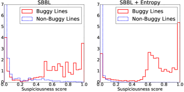
(a) Defects4J dataset

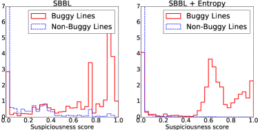
(b) ManyBugs dataset

Figure 6: Histogram of suspiciousness score per source code lines. $x$-axis shows suspiciousness score given by equation 6 and the $y$-axis is the relative frequency.

The results are shown in the bottom table of Figure 5. For all the projects we studied, AUCEC₁₀₀ increases when we incorporate entropy related features, with an overall gain of 6.617% (3.81% and 9.11% for Defects4J and ManyBugs dataset respectively). The positive gain indicates that ${\cal L}{\cal M}$ can indeed improve the performance of ${\cal S}{\cal B}{\cal B}{\cal L}$ bug localization. Top three features (sorted based on their importance learned by Random Forest algorithm in the training phase) are also reported as Feature1, Feature2 and Feature3. For all the cases, Average Entropy is the most important feature. Thus, we conclude that, entropy plays the most important role in localizing bugs for EnSpec.

Next, we check how EnSpec performs with ${\cal S}{\cal B}{\cal B}{\cal L}$ + entropy related features over ${\cal S}{\cal B}{\cal B}{\cal L}$ only features while inspecting small portion of source code lines (SLOC), as that is more realistic scenario. Figure 5(a) shows the overall effect of entropy across all the projects at an inspection budget of 20%. With ${\cal S}{\cal B}{\cal B}{\cal L}$ only features, we can detect only 80.08% of total buggy lines (AUCEC₂₀ is 0.10475). However, with ${\cal S}{\cal B}{\cal B}{\cal L}$ + entropy features, we can detect 98.63% buggy lines (AUCEC₂₀ is 0.13966). Thus we see an overall gain of 33.33% in AUCEC₂₀ with entropy.

Next, we check, at a even lower inception budget, how EnSpec performs. Figure 5(b) and Figure 5(c) shows the cost-effectiveness curve for individual projects in Defects4J and ManyBugs dataset respectively. Here, ${\cal S}{\cal B}{\cal B}{\cal L}$ + entropy yields better performance over ${\cal S}{\cal B}{\cal B}{\cal L}$ only setting for all the projects except two: for Apache commons-math both performs almost equal and for Libtiff, EnSpec performs worse.

We further investigate, why ${\cal L}{\cal M}$ is helping ${\cal S}{\cal B}{\cal B}{\cal L}$ to improve bug localization. Figure 6(a) and 6(b) show the histogram of suspiciousness scores per line from Defects4J and ManyBugs dataset in both the settings. For ${\cal S}{\cal B}{\cal B}{\cal L}$ only setting, a large proportion of actual non-buggy lines (marked in blue) lie in the higher suspiciousness score range. So, those non-buggy lines are ranked in higher position than the buggy lines (marked in red) having lower scores, lowering down the overall bug-localization performance. But, in ${\cal S}{\cal B}{\cal B}{\cal L}$ + Entropy setting, the proportion of non-buggy lines having higher hybrid suspiciousness scores decreases, improving the overall bug localization performance.

Result 5.5: Entropy, as derived by statistical language model, improved bug localization capabilities of ${\cal S}{\cal B}{\cal B}{\cal L}$.

For projects with smaller size and less number of test cases, EnSpec might not work well, since smaller projects do not have enough bug data to train EnSpec. To mitigate this threat, we now evaluate EnSpec’s performance in cross-project settings.

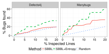
(a) Bug localization performance with an inspection budget of 20% of total lines. 75.34% and 54.5% gain in the corresponding AUCEC values for Defects4J and ManyBugs projects respectively, when we use entropy.

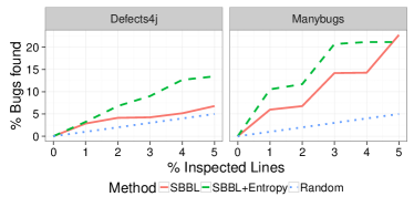
(b) Bug localization performance with an inspection budget of 5% of total lines. 94.16% and 54.18% gain in the corresponding AUCEC values for Defects4J and ManyBugs projects respectively, when we use entropy.

Dataset	Project	AUCEC100	AUCEC100	Overall Gain	Top Three Features
		(${\cal S}{\cal B}{\cal B}{\cal L}$ only)	(${\cal S}{\cal B}{\cal B}{\cal L}$ + entropy)	(%)	Feature1	Feature2	Feature3
	JFreechart	0.878	0.955	8.882	Average entropy	Hamming	Euclid
	Closure compiler	0.681	0.816	37.796	Average entropy	Ample	RusselRao
Defects4J	Apache commons-lang	0.619	0.840	36.655	Average entropy	Euclid	RogersTanimoto
	Apache commons-math	0.743	0.774	4.172	Mean entropy	Euclid	Hamming
	Joda-Time	0.662	0.794	19.939	Average entropy	Hamming	Sokal
	Average	0.717	0.836	16.59
	Libtiff	0.565	0.729	45.026	Average entropy	Wong3	RogersTanimoto
	Lighttpd	0.616	0.848	37.623	Average entropy	RogersTanimoto	SimpleMatching
ManyBugs	Php	0.508	0.541	11.299	Mean entropy	Wong3	Hamming
	Python	0.577	0.792	37.422	Average entropy	Ample	Euclid
	Wireshark	0.757	0.898	20.489	Average entropy	RogersTanimoto	Sokal
	Average	0.605	0.762	25.95

Figure 7: Overall performance of EnSpec (${\cal S}{\cal B}{\cal B}{\cal L}$ + Entropy) vs. ${\cal S}{\cal B}{\cal B}{\cal L}$ in cross project setting.

RQ3. What is the effect of entropy on ${\cal S}{\cal B}{\cal B}{\cal L}$’s bug localization capability in a cross-project setting?

To answer this research question, we first build a cross-project ${\cal L}{\cal M}$. To train the ${\cal L}{\cal M}$ for a given buggy project version, v_target, we select all the other buggy versions (v_train) from different projects with the following two constraints: (1) v_train and v_target are written in the same language, and (2) v_train are created before $v_{target}$. The first constraint ensures that the ${\cal L}{\cal M}$ is trained on the same programming language specific features and usages. Thus, for a given Java project, ${\cal L}{\cal M}$ only learns from other Java projects from Defects4J dataset. Similarly, for a C project, we choose other C projects from ManyBugs dataset for training.

The second constraint emulates the real world scenario: to train a ${\cal L}{\cal M}$ for v_target, the training set (v_train) has to be available in the first place. Hence, we organize different project versions of a dataset chronologically, based on their last commit date, as retrieved from version repository. Then, for v_target, we choose all the versions from different projects that are chronologically appeared before v_target. Thus, for both the dataset, we choose a buggy version as the target if there exists at least one previous buggy version from another project.

Next, for each v_target, we train EnSpec based on the features of v_train. Similar to our previous experiments, the features include entropy scores generated by $gram+type language model (see equation 3), and 25 ${\cal S}{\cal B}{\cal B}{\cal L}$ specific suspiciousness scores, for each program line. Based on the training, EnSpec then assigns a suspiciousness score per line in the test data, v_target, indicating the line’s likelihood of being buggy. Finally, we rank the lines with decreasing order of their suspiciousness score—line with the highest value tops the list. To evaluate the performance of EnSpec at cross-project setting, we calculate the AUCEC_n score, which basically tells us the rate and the percentages of bugs that can be found if a developer inspects n% lines in the ranked-list returned by the tool. We also repeat the experiment without entropy as a feature, i.e. with only ${\cal S}{\cal B}{\cal B}{\cal L}$ suspiciousness score. As a baseline, we report the percentage of buggy lines found at an inspection budget of n, while we randomly choose n% lines from source code. Figure 7 shows the results.

Figure 7(a) shows that if developers inspect top 20% of source code lines, following ${\cal S}{\cal B}{\cal B}{\cal L}$ +Entropy ranking scheme, 33.54% and 59.65% of the buggy lines are detected for Defects4J and ManyBugs respectively. In contrast, when we use only ${\cal S}{\cal B}{\cal B}{\cal L}$ based ranking scheme, 19.24% and 35.72% buggy lines can be detected for Defects4J and ManyBugs respectively. Thus, we see an overall gain of 75.34% and 54.5% of AUCEC₂₀, when we include entropy in the feature set. Note that, this gain even increases at a stricter inspection budget for Defects4J projects—Figure 7(b) reports an overall gain of 94.16% in AUCEC₅. For ManyBugs, we see a gain of 54.18%, which is similar to AUCEC₂₀ gain. Both ranking schemes perform better than random.

The table at bottom in Figure 7 shows AUCEC₁₀₀ values achieved by two strategies for each project at an inspection budget of 100. In both cases, developers would find 100% of buggy lines since they inspect all the lines in the ranked list. However, the rate of identifying 100% of buggy lines is higher using EnSpec than ${\cal S}{\cal B}{\cal B}{\cal L}$ only. Result shows that EnSpec has 16.59% performance gain for Defects4J data set, and 25.95% gain for ManyBugs, on average. As discussed earlier, including entropy as a feature benefits bug localization even more at lower inspection budget, which is a more realistic scenario.

We further check the relative importance of the features learned by EnSpec (last three columns of the Table in Figure 7 lists the three most important features). Interestingly, in all the cases, entropy exhibits highest importance than any ${\cal S}{\cal B}{\cal B}{\cal L}$ based features. The above results show that a good ${\cal L}{\cal M}$ can significantly improve ${\cal S}{\cal B}{\cal B}{\cal L}$ in a cross-project bug localization setting.

Result 5.5: Entropies derived from ${\cal L}{\cal M}$ significantly improves bug localization capabilities of ${\cal S}{\cal B}{\cal B}{\cal L}$ in a cross-project setting.

7 Related Work

Automatic bug localization has been an active research area over two decades. Existing techniques can be broadly classified into two broad categories: i) static and ii) dynamic approaches.

Static approaches primarily rely on program source code. There are mainly two kinds of static approaches: a) program analysis based approaches, and b) information retrieval (IR) based approaches. Program analysis based approaches detect bugs by identifying well-known buggy patterns that frequently happened in practice. Therefore, although these approaches are effective in preventing bugs by enforcing good programming practices, they generally cannot detect functional bugs. FindBugs [5] is a popular example in this category. On the other hand, IR-based approaches, given a bug report, generally rank source code files based on the textual similarity between source code and the bug report so that potential buggy files ranked high in the ranked-list. These approaches are generally fast but identify bugs at coarse grained level. BugLocator [60], BLUiR [48] are some of the examples in this category.

There is a new line of work that recently started based on statistical modeling and machine learning. Wang et al.[55] proposed a Deep Belief Network based approached to detect file level defects. Wang et al.[54] used n-gram language model to generate a list of probable bugs.

Dynamic approaches generally rely on the execution traces of test cases. ${\cal S}{\cal B}{\cal B}{\cal L}$ is a dynamic fault localization technique that leverages program spectra—program paths executed by passed and failed test cases [47] to compute a suspiciousness score of each program element. We have described ${\cal S}{\cal B}{\cal B}{\cal L}$ in detail in Section 2.1. Several metrics have been proposed in the literature to calculate the suspiciousness score. For example, Jones et al.presented Tarantula [30] based on the fact that program elements executed by failed test cases are more likely to bug than the elements not executed by them (see Table 1). Jaccard and Ochiai are some of the well known variants of this approach proposed by Abreu et al. [3]. Xie et al.proposed five ranking metrics by theoretical analysis and four other metrics based on genetic algorithms [56]. Later, Lucia et al.did a comprehensive study of the different ranking metrics and showed that no ranking metric is unanimously best [39]. ${\cal S}{\cal B}{\cal B}{\cal L}$ approaches can identify bugs at fine-grained level.

Xuan et al. [57] proposed an approach to combine multiple ranking metrics. They adopted neighborhood based strategy to reduce the imbalance ratio of buggy and non-buggy program entities. For their algorithm, they need an initial metric to define the neighborhood. They sort the data based on an initial ranking metric. The filtered $\beta$ non-faulty entities before and after a faulty entity. After that, they applied state of the art "Learning to Rank" algorithms to combine all 25 suspiciousness scores. Their dependence on an initial ranking metric might cause a bias towards that metric. In contrast, to be unbiased to any of the metric, we considered all the data and applied state of the art random under-sampling[7] technique.

Gong et al. [23] proposed a feedback based fault localization system, which uses user feedback to improve performance. Pytlik et al. [42] proposed the fault localization system using the likely invariant. Le et al.[6] also proposed an approach similar to Pytlic et al. with a larger invariant set. Unlike this work, they experimented on method level fault localization system. Sahoo et al. extended Pytlik et al’s work. Their work is on test case generation and also they adopted backward slicing to reduce the number of program element to be considered.

Multi-modal techniques generally combine two or more model of bug localization to improve the accuracy further. Le et al. [33] proposed a multi-modal technique for bug localization that basically combines the IR and spectrum based bug localization together. Their technique needs three artifacts: i) a bug report, ii) program source code, and iii) a set of test cases having at least a fault reproducing test case. Their technique first rank the source code methods based on the textual similarity between bug report and source code methods. Then using program spectra, they rank the source code lines and also identifies a list of suspicious words associated with the bug. Finally they combine these scores using a probabilistic model which is trained on a set of previously fixed bugs. Based on an empirical evaluation on 157 real bugs from four software systems, their model outperforms a state-of-the-art IR-based bug localization technique, a state-of-the-art spectrum-based bug localization technique, and three state-of-the-art multi-modal feature location methods that are adapted for bug localization.

The proposed approach in this paper is also multi-modal in nature. However, instead of combining IR-based textual similarity score,inspired by Ray et al.’s[45] finding that the buggy codes are unnatural, and thus entropy of a buggy source code is naturally high, we combine source code entropy with program spectra to improve bug localization. To our knowledge, no one leveraged the localness of code and test spectrum together to locate faults. The advantage of our approach is that we do not need any bug report which may not be available for development bugs. Therefore, our approach is complementary to Le et al’s approach.

8 Threats to Validity

Efficiency of EnSpec depends on the availabity of previous bugs on which the model will be trained. To minimize this threat, we demonstrated that EnSpec works well in cross-project setting.

EnSpec is also dependent on the adequecy of the test suite. If there are not enough failing test cases, performance of ${\cal S}{\cal B}{\cal B}{\cal L}$ may get hurt, and hence EnSpec’s performance will also be worse. However, since EnSpec is a hybrid approach, it does not solely depend on test suites. The ${\cal L}{\cal M}$ based part will still be able to locate bugs since the latter does not require anything but source code.

Further, to annotate buggy lines, we rely on the publicly available bug-dataset and some evolutionary bugs. It can be possible there are other bugs lying in the code corpus that are polluting our results. However, at any given point of time it is impossible to know the presence of all the bugs in a software.

Finally, to minimize threats due to external validity, we evaluated EnSpec on 10 projects for 2 languages: C and Java. This proves, EnSpec is not restricted to any particular programming language.

9 Conclusion

While spectrum based bug localization is an extensively studied research area, studying buggy code in association with code naturalness (thus unnaturalness) is relatively new. In this work, we introduced the notion of code entropy as captured by statistical language model in ${\cal S}{\cal B}{\cal B}{\cal L}$ to make the overall bug localization more robust, and proposed an effective way of integrating entropy with ${\cal S}{\cal B}{\cal B}{\cal L}$ suspicious scores. We implemented our concept in a prototype called EnSpec. Our experimental results with EnSpec show that code entropy is positively correlated with the buggy lines executed by the failing test cases. Our results also demonstrate that EnSpec, when configured to use both entropy and ${\cal S}{\cal B}{\cal B}{\cal L}$, outperforms the configuration that uses only various ${\cal S}{\cal B}{\cal B}{\cal L}$ as features. EnSpec can also be leveraged for detecting bugs in cross-project setting for relatively new projects, where project bug database and evolutionary history is not strong enough.

Our future direction includes leveraging EnSpec to repair buggy program line more effectively, and improving EnSpec further by incorporating language model which captures not only the syntactic structure but also code semantic structure.

References

- [1] Ranklib (https://sourceforge.net/p/lemur/wiki/RankLib/). https://sourceforge.net/p/lemur/wiki/RankLib/.
- [2] R. Abreu, P. Zoeteweij, R. Golsteijn, and A. J. Van Gemund. A practical evaluation of spectrum-based fault localization. Journal of Systems and Software, 82(11):1780–1792, 2009.
- [3] R. Abreu, P. Zoeteweij, and A. J. Van Gemund. On the accuracy of spectrum-based fault localization. In Testing: Academic and Industrial Conference Practice and Research Techniques-MUTATION, 2007. TAICPART-MUTATION 2007, pages 89–98. IEEE, 2007.
- [4] E. Arisholm, L. C. Briand, and E. B. Johannessen. A systematic and comprehensive investigation of methods to build and evaluate fault prediction models. Journal of Systems and Software, 83(1):2–17, 2010.
- [5] N. Ayewah, D. Hovemeyer, J. D. Morgenthaler, J. Penix, and W. Pugh. Using static analysis to find bugs. IEEE software, 25(5), 2008.
- [6] T.-D. B Le, D. Lo, C. Le Goues, and L. Grunske. A learning-to-rank based fault localization approach using likely invariants. In Proceedings of the 25th International Symposium on Software Testing and Analysis, pages 177–188. ACM, 2016.
- [7] G. E. Batista, R. C. Prati, and M. C. Monard. A study of the behavior of several methods for balancing machine learning training data. ACM Sigkdd Explorations Newsletter, 6(1):20–29, 2004.
- [8] L. Breiman. Random forests. Machine learning, 45(1):5–32, 2001.
- [9] P. F. Brown, P. V. Desouza, R. L. Mercer, V. J. D. Pietra, and J. C. Lai. Class-based n-gram models of natural language. Computational linguistics, 18(4):467–479, 1992.
- [10] L. Buitinck, G. Louppe, M. Blondel, F. Pedregosa, A. Mueller, O. Grisel, V. Niculae, P. Prettenhofer, A. Gramfort, J. Grobler, R. Layton, J. VanderPlas, A. Joly, B. Holt, and G. Varoquaux. API design for machine learning software: experiences from the scikit-learn project. In ECML PKDD Workshop: Languages for Data Mining and Machine Learning, pages 108–122, 2013.
- [11] J. C. Campbell, A. Hindle, and J. N. Amaral. Syntax errors just aren’t natural: improving error reporting with language models. In Proceedings of the 11th Working Conference on Mining Software Repositories, pages 252–261. ACM, 2014.
- [12] N. V. Chawla, N. Japkowicz, and A. Kotcz. Editorial: special issue on learning from imbalanced data sets. ACM Sigkdd Explorations Newsletter, 6(1):1–6, 2004.
- [13] B. Chelf, D. Engler, and S. Hallem. How to write system-specific, static checkers in metal. In Proceedings of the 2002 ACM SIGPLAN-SIGSOFT Workshop on Program Analysis for Software Tools and Engineering, PASTE ’02, pages 51–60, New York, NY, USA, 2002. ACM.
- [14] H. Cleve and A. Zeller. Locating causes of program failures. In Software Engineering, 2005. ICSE 2005. Proceedings. 27th International Conference on, pages 342–351. IEEE, 2005.
- [15] T. Copeland. PMD applied. Centennial Books San Francisco, 2005.
- [16] M. D’Ambros, M. Lanza, and R. Robbes. An extensive comparison of bug prediction approaches. In Mining Software Repositories (MSR), 2010 7th IEEE Working Conference on, pages 31–41. IEEE, 2010.
- [17] T. G. Dietterich. Ensemble learning. The handbook of brain theory and neural networks, 2:110–125, 2002.
- [18] D. Engler, D. Y. Chen, S. Hallem, A. Chou, and B. Chelf. Bugs as deviant behavior: A general approach to inferring errors in systems code. In Proceedings of the Eighteenth ACM Symposium on Operating Systems Principles, SOSP ’01, pages 57–72, New York, NY, USA, 2001. ACM.
- [19] FindBugs. http://findbugs.sourceforge.net/. Accessed 2015/03/10.
- [20] C. Franks, Z. Tu, P. Devanbu, and V. Hellendoorn. Cacheca: A cache language model based code suggestion tool. In ICSE Demonstration Track, 2015.
- [21] Y. Freund, R. Iyer, R. E. Schapire, and Y. Singer. An efficient boosting algorithm for combining preferences. Journal of machine learning research, 4(Nov):933–969, 2003.
- [22] M. Gabel and Z. Su. A study of the uniqueness of source code. In Proceedings of the eighteenth ACM SIGSOFT international symposium on Foundations of software engineering, pages 147–156. ACM, 2010.
- [23] L. Gong, D. Lo, L. Jiang, and H. Zhang. Interactive fault localization leveraging simple user feedback. In Software Maintenance (ICSM), 2012 28th IEEE International Conference on, pages 67–76. IEEE, 2012.
- [24] U. Gunneflo, J. Karlsson, and J. Torin. Evaluation of error detection schemes using fault injection by heavy-ion radiation. In Fault-Tolerant Computing, 1989. FTCS-19. Digest of Papers., Nineteenth International Symposium on, pages 340–347. IEEE, 1989.
- [25] V. J. Hellendoorn, P. T. Devanbu, and A. Bacchelli. Will they like this?: evaluating code contributions with language models. In Proceedings of the 12th Working Conference on Mining Software Repositories, pages 157–167. IEEE Press, 2015.
- [26] A. Hindle, E. Barr, M. Gabel, Z. Su, and P. Devanbu. On the naturalness of software. In ICSE, pages 837–847, 2012.
- [27] A. Hindle, E. T. Barr, Z. Su, M. Gabel, and P. Devanbu. On the naturalness of software. In 2012 34th International Conference on Software Engineering (ICSE), pages 837–847. IEEE, 2012.
- [28] N. Japkowicz and S. Stephen. The class imbalance problem: A systematic study. Intelligent data analysis, 6(5):429–449, 2002.
- [29] B. Johnson, Y. Song, E. Murphy-Hill, and R. Bowdidge. Why don’t software developers use static analysis tools to find bugs? In Software Engineering (ICSE), 2013 35th International Conference on, pages 672–681. IEEE, 2013.
- [30] J. A. Jones and M. J. Harrold. Empirical evaluation of the tarantula automatic fault-localization technique. In Proceedings of the 20th IEEE/ACM international Conference on Automated software engineering, pages 273–282. ACM, 2005.
- [31] J. A. Jones, M. J. Harrold, and J. Stasko. Visualization of test information to assist fault localization. In Proceedings of the 24th international conference on Software engineering, pages 467–477. ACM, 2002.
- [32] R. Just, D. Jalali, and M. D. Ernst. Defects4j: A database of existing faults to enable controlled testing studies for java programs. In Proceedings of the 2014 International Symposium on Software Testing and Analysis, pages 437–440. ACM, 2014.
- [33] T.-D. B. Le, R. J. Oentaryo, and D. Lo. Information retrieval and spectrum based bug localization: better together. In Proceedings of the 2015 10th Joint Meeting on Foundations of Software Engineering, pages 579–590. ACM, 2015.
- [34] C. Le Goues, N. Holtschulte, E. K. Smith, Y. Brun, P. Devanbu, S. Forrest, and W. Weimer. The manybugs and introclass benchmarks for automated repair of c programs. IEEE Transactions on Software Engineering, 41(12):1236–1256, 2015.
- [35] C. Le Goues, W. Weimer, and S. Forrest. Representations and operators for improving evolutionary software repair. In Proceedings of the 14th annual conference on Genetic and evolutionary computation, pages 959–966. ACM, 2012.
- [36] P. Li, C. J. Burges, Q. Wu, J. Platt, D. Koller, Y. Singer, and S. Roweis. Mcrank: Learning to rank using multiple classification and gradient boosting. In NIPS, volume 7, pages 845–852, 2007.
- [37] B. Liblit, M. Naik, A. X. Zheng, A. Aiken, and M. I. Jordan. Scalable statistical bug isolation. ACM SIGPLAN Notices, 40(6):15–26, 2005.
- [38] C. Liu, X. Yan, L. Fei, J. Han, and S. P. Midkiff. Sober: statistical model-based bug localization. In ACM SIGSOFT Software Engineering Notes, volume 30, pages 286–295. ACM, 2005.
- [39] L. Lucia, D. Lo, L. Jiang, F. Thung, and A. Budi. Extended comprehensive study of association measures for fault localization. Journal of Software: Evolution and Process, 26(2):172–219, 2014.
- [40] H. B. Mann and D. R. Whitney. On a test of whether one of two random variables is stochastically larger than the other. The annals of mathematical statistics, pages 50–60, 1947.
- [41] A. Mockus and L. G. Votta. Identifying reasons for software changes using historic databases. In icsm, pages 120–130, 2000.
- [42] B. Pytlik, M. Renieris, S. Krishnamurthi, and S. P. Reiss. Automated fault localization using potential invariants. arXiv preprint cs/0310040, 2003.
- [43] F. Rahman, S. Khatri, E. T. Barr, and P. Devanbu. Comparing static bug finders and statistical prediction. In Proceedings of the 36th International Conference on Software Engineering, pages 424–434. ACM, 2014.
- [44] S. Rao and A. Kak. Retrieval from software libraries for bug localization: a comparative study of generic and composite text models. In Proceedings of the 8th Working Conference on Mining Software Repositories, pages 43–52. ACM, 2011.
- [45] B. Ray, V. Hellendoorn, S. Godhane, Z. Tu, A. Bacchelli, and P. Devanbu. On the naturalness of buggy code. In Proceedings of the 38th International Conference on Software Engineering, pages 428–439. ACM, 2016.
- [46] V. Raychev, M. Vechev, and E. Yahav. Code completion with statistical language models. In PLDI, pages 419–428, 2014.
- [47] T. Reps, T. Ball, M. Das, and J. Larus. The use of program profiling for software maintenance with applications to the year 2000 problem. In Software Engineering—ESEC/FSE’97, pages 432–449. Springer, 1997.
- [48] R. K. Saha, M. Lease, S. Khurshid, and D. E. Perry. Improving bug localization using structured information retrieval. In Automated Software Engineering (ASE), 2013 IEEE/ACM 28th International Conference on, pages 345–355. IEEE, 2013.
- [49] Z. Segall, D. Vrsalovic, D. Siewiorek, D. Ysskin, J. Kownacki, J. Barton, R. Dancey, A. Robinson, and T. Lin. Fiat-fault injection based automated testing environment. In Fault-Tolerant Computing, 1995, Highlights from Twenty-Five Years., Twenty-Fifth International Symposium on, page 394. IEEE, 1995.
- [50] J. Śliwerski, T. Zimmermann, and A. Zeller. When do changes induce fixes? In ACM sigsoft software engineering notes, volume 30, pages 1–5. ACM, 2005.
- [51] Z. Tu, Z. Su, and P. Devanbu. On the localness of software. In SIGSOFT FSE, pages 269–280, 2014.
- [52] Z. Tu, Z. Su, and P. Devanbu. On the localness of software. In Proceedings of the 22nd ACM SIGSOFT International Symposium on Foundations of Software Engineering, pages 269–280. ACM, 2014.
- [53] J. Walden, J. Stuckman, and R. Scandariato. Predicting vulnerable components: Software metrics vs text mining. In Software Reliability Engineering (ISSRE), 2014 IEEE 25th International Symposium on, pages 23–33. IEEE, 2014.
- [54] S. Wang, D. Chollak, D. Movshovitz-Attias, and L. Tan. Bugram: bug detection with n-gram language models. In Proceedings of the 31st IEEE/ACM International Conference on Automated Software Engineering, pages 708–719. ACM, 2016.
- [55] S. Wang, T. Liu, and L. Tan. Automatically learning semantic features for defect prediction. In Proceedings of the 38th International Conference on Software Engineering, pages 297–308. ACM, 2016.
- [56] X. Xie, T. Y. Chen, F.-C. Kuo, and B. Xu. A theoretical analysis of the risk evaluation formulas for spectrum-based fault localization. ACM Transactions on Software Engineering and Methodology (TOSEM), 22(4):31, 2013.
- [57] J. Xuan and M. Monperrus. Learning to combine multiple ranking metrics for fault localization. In ICSME-30th International Conference on Software Maintenance and Evolution, 2014.
- [58] X. Ye, R. Bunescu, and C. Liu. Learning to rank relevant files for bug reports using domain knowledge. In Proceedings of the 22nd ACM SIGSOFT International Symposium on Foundations of Software Engineering, pages 689–699. ACM, 2014.
- [59] A. Zeller and R. Hildebrandt. Simplifying and isolating failure-inducing input. IEEE Transactions on Software Engineering, 28(2):183–200, 2002.
- [60] J. Zhou, H. Zhang, and D. Lo. Where should the bugs be fixed?-more accurate information retrieval-based bug localization based on bug reports. In Proceedings of the 34th International Conference on Software Engineering, pages 14–24. IEEE Press, 2012.
- [61] D. W. Zimmerman. Comparative power of student t test and mann-whitney u test for unequal sample sizes and variances. The Journal of Experimental Education, 55(3):171–174, 1987.
- [62] T. Zimmermann, N. Nagappan, H. Gall, E. Giger, and B. Murphy. Cross-project defect prediction: a large scale experiment on data vs. domain vs. process. In Proceedings of the the 7th joint meeting of the European software engineering conference and the ACM SIGSOFT symposium on The foundations of software engineering, pages 91–100. ACM, 2009.