Electron emission by long and short wavelength lasers: essentials for the design of plasmonic photocathodes

Abstract

Theory of electron emission by metallic photocathodes under the exposure of long wavelength lasers will be studied. Energy of photons in long wavelength lasers is less than the work function of the photocathode’s material, and can only emit electrons via tunneling through the potential barrier. The optical resonance effect (e.g. plasmonic resonances) will be studied as an improvement to the performance of photocathodes. This paper is intended to provide self-sufficient materials to design optical resonant surfaces (e.g. metasurfaces) for electron emission applications.

I Introduction

Electromagnetic interaction, one of the four known fundamental forces in the universe, was proposed by Michael Faraday in 1820’s Faraday (1834), theorized by James Clerk Maxwell in 1865 Maxwell (1881), and experimentally proved by Heinrich Hertz in 1888 Hertz (1893). Since then, developed sources of electromagnetic waves are based on moving (ideally resonating) electrons either in free space or inside a material (e.g. semiconductors). In fact, less than four decades after the discovery of electromagnetism, in 1924, Louis de Broglie suggested that moving particles such as electrons behave as waves with frequencies related to their momentums De Broglie (1923). Modern and traditional high power electromagnetic sources such as magnetrons and Klystrons (developed during WWII by the Allied and the Axis Powers, respectively) are based on extracting electrons into vacuum (electron emission), bunching them, modulating their speed, and extracting their energy to an output electromagnetic wave. In other words, although transistors were invented more than half a century ago, modern solid state microwave sources are still inferior to their electron beam-based rivals at least in terms of the power level. A solid state source is roughly limited to less than a MW peak power while an electron beam-based source can provide GW ranges Schamiloglu (2004). This seems obvious since semiconductors (and generally any material) impose their limitations such as speed, bandgap, loss, etc. to the designed device. As a matter of fact, residing electrons in vacuum, prior to their manipulation, is the extreme of relaxing most limitations of solid state devices. This signifies the importance and profundity of electron emission and its great potentials.

Traditionally, thermal emission used to be the dominant method of electron emission in engineering devices, which was followed by electric field emission, photoemission, and even emission by another electron beam (a.k.a. secondary emission). For the sake of self consistency, we review these physics and their common formulations in the next section, prior to discussing photoemission at long wavelength. The main contribution in this paper is to formulate photoemission by photons with energies lower than the photocathode’s work function (e.g. infrared (IR) laser illuminating gold photocathodes). Our motivation for this study is the potential that we see in engineered resonant surfaces (a.k.a. metasurfaces) for IR photocathode applications. Such photocathodes can be useful at least for two purposes:

a) IR photocathodes can be used to generate a cloud of free electrons for microelectronic applications in order to circumvent semiconductors limitations. For a semiconductor-free microelectronic device, IR is much preferred over the usual ultraviolet (UV) light for a photocathode, due to safety concerns. Moreover, metallic metasurfaces at IR can leverage plasmoinc resonance effects to enhance the photon-electron interaction significantly, which can reduce the light intensity requirement down into the safe range. We reported an example of such devices in Forati et al. (2016), where the continuous wave (CW) IR radiation of a mW diode laser generated observable electron emission using a properly designed plasmonic metasurface.

b) metasurfaces are, in general, designed to manipulate/control the phase front of the reflected wave from their surface Sievenpiper et al. (2003). If the metasurface itself is also the electron emitter, the correlation between the incoming photons and emitted electrons may be maintained to some extent. This may provide an opportunity to control the phase front of the emitted electron beam (considering De Broglie wave picture for electrons). Obviously, this possible application is not limited to the IR range, but the ability to leverage plasmonic resonances on noble metals makes the IR range more attractive.

Nonetheless, there are stablished theories for UV photoemission as we will review later in this paper. Photocathodes have advanced applications such as in Linear accelerators (to convert photon bunches into electron bunches), x-ray sources, high energy colliders, and free electron lasers (FELs) where short electron bunches are necessary. An FEL generates coherent light due to the interaction of a train of electron bunches and light waves. Important quantifying parameters of photocathodes are quantum efficiency (QE), survivability, emission promptness, lifetime, and emittance, among which QE is extremely important since it is accessible experimentally. QE is defined as Jensen et al. (2005)

$$QE=\frac{\hbar\omega}{q}\left(\frac{J_{\mathrm{e}}}{I_{\mathrm{\lambda}}}\right)=1.2398\frac{J_{\mathrm{e}}\left(A/cm^{2}\right)}{I_{\mathrm{\lambda}}\left(W/cm^{2}\right)\lambda\left(nm\right)},$$ (1)

in which q is the elementary charge, $\omega$ is the radial frequency, $\hbar$ is the reduced Plank’s constant, $J_{\mathrm{e}}$ and $I_{\mathrm{\lambda}}$ are electric current and optical intensity, respectively (units are given in the parenthesis). An example of a photocathode requirements for FEL application is $0.1-1\,$A current arranged in $0.1-1\,$ nC bunches in $10-50\,$ps pulses with GHz repetition rates in applied fields of $10-50\,$MV/m Jensen et al. (2006). The speed requirement rules out thermionic emitters for FELs since they cannot switch current in picosecond time scales. In general, an electron beam with a lower spatial divergence (emittance) and a higher current (brightness) can provide shorter wavelength and more powerful FELs.

Both metals and semiconductors are popular for photocathodes. Metallic photocathodes have more ruggedness, lower QE, and faster response (which makes them suitable for pulse shaping). Metallic photocathodes usually require UV light for emission, which normally is considered as a restriction because UV is usually generated by nonlinear conversion of 1064 nm Nd:YAG with low conversion efficiencies. On the other hand, semiconductor photocathodes have higher QE, but are chemically reactive and can be easily damaged by carbon dioxide or water. They also have slower response time (larger than 40 ps) compared to their metallic counterparts. Examples of semiconductor photocathodes are direct bandgap p-type semiconductors including III-V with cesium and oxidant, alkali antimonides, and alkali tellurides Jensen et al. (2006). A usual solution for combining benefits of rugged materials with high QE materials is to design dispenser photocathodes, in which a low work function material such as Barium diffuses out from a porous material with higher ruggedness (e.g. tungsten). High vacuums (on the order of 1e-9 Torr) are usually needed for metallic photocathodes, and the requirement becomes more strict for semiconductor photocathodes.

Although approaches are similar, the physics of photoemission from semiconductor and metallic photocathodes are different in their electron distribution (e.g. bandgap) and transport (e.g. scattering mechanisms). In this paper, we only consider metallic photocathodes although sum of the discussions apply to semiconductor photocathodes as well. As a result, Fermi-Dirac model for electrons distribution is used throughout this paper. The arguments in this paper are valid for both CW or pulsed laser excitations.

II Thermal and electric field emission theories

Four major identified methods of electron emission are thermal emission, electric field emission, photoemission, and emission by other high energy electrons (which is called secondary emission and is beyond the subject of this paper). A photocathode (despite its name implication) usually involves all three mechanisms. That is, usually a bias voltage is applied to the photocathode, and usually the applied laser pulse causes thermal heating of the photocathode. The canonical equations governing thermal emission, field emission, and photoemission are Richardson-Laue-Dushman, Fowler-Nordheim, and Fowler-Dubridge, respectively. In order to start reviewing the three methods, consider the potential diagram of a metal-vacuum interface as shown in Fig. 1.

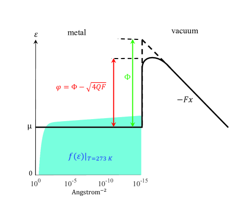
Figure 1: The potential barrier with Shottkey lowering effect. The supply function of gold with $\mu=$5.53 eV at T=273 K is also shown.

The chemical potential of electrons in the metal and the work function are identified by $\mu$ and $\Phi,$ respectively. If a static electric field $\left(E_{\mathrm{static}}\right)$ is applied on the metal surface, the work function will be reduced to Dowell and Schmerge (2009); Gadzuk and Plummer (1973)

$$\phi=\Phi-\sqrt{4QF_{\mathrm{static}}}$$ (2)

in which $F_{\mathrm{static}}=qE_{\mathrm{static}}$, and $Q=q^{2}/\left(16\pi\varepsilon_{0}\right)=0.35999$ eV nm. The parameter $\phi$ is referred to as Shottkey reduced boundary condition, and it includes the charge image effect of the metal on the potential energy outside the metal (the same well-known image theorem in electromagnetism). Since we only discuss metallic photocathodes (with free electrons which are indeed Fermions), Fermi-Dirac distribution is usually considered for electrons inside the metal and the number density of electrons is given by Jensen (2017)

$$\rho=\frac{2}{\left(2\pi\right)^{3}}\iiint\frac{dk}{1+exp\left(\beta_{\mathrm{T}}\left(\varepsilon-\mu\right)\right)},$$ (3)

where k is electron momentum and is related to its energy $\left(\varepsilon\right)$ by $\varepsilon=\hbar^{2}k^{2}/2m.$ The parameter $\beta_{\mathrm{T}}=1/k_{\mathrm{B}}T$ is sometimes called the thermal slope factor, in which $T$ is the temperature in Kelvin unit and $k_{\mathrm{B}}$ is Boltzmann’s constant. Equation (3) includes electrons with momentums in every direction, however we are only interested in electrons with momentums normal to the metal surface. It is straight forward to show that integration of (3) over parallel momentums to the metal surface leads to Jensen (2017)

$$f\left(\varepsilon\right)=\frac{m}{\pi\hbar^{2}\beta_{\mathrm{T}}}ln\left\{1+exp\left[\beta_{\mathrm{T}}\left(\mu-\varepsilon\right)\right]\right\}$$ (4)

which is called the supply function in electron emission theories. In fact, (4) is the number density of electrons with momentums normal to the surface $\left(f\left(\varepsilon_{\bot}=\hbar^{2}k_{\bot}^{2}/2m\right)\right),$ which we dropped the subscript $\bot$ for convenience throughout the rest of this paper. Figure 1 also includes the supply function of gold with $\mu=5.53\,$eV at T=273 K.

The current density normal to the metal surface can be written as Jensen (2017)

$$J=q\rho v=\frac{2q}{2\pi}\int\left(\frac{\hbar k}{m}\right)f\left(\varepsilon\right)T\left(\varepsilon\right)dk$$ (5)

$$\quad=\frac{q}{2\pi\hbar}\intop_{0}^{\infty}T\left(\varepsilon\right)f\left(\varepsilon\right)d\varepsilon,$$

in which $v=\hbar k/m$ is the speed of electrons, $T\left(\varepsilon\right)$ is the probability of an electron passing the barrier, and the factor of 2 in the numerator accounts for the spin.

In the event of a thermal emission, Richardson approximation is used, where Heaviside step function is used for $T\left(\varepsilon\right)$ as

$$T\left(\varepsilon\right)=\begin{cases}\begin{array}[]{c}1\\ 0\end{array}&\begin{array}[]{c}\varepsilon>\phi\\ \varepsilon<\phi\end{array}\end{cases}.$$ (6)

This leads to the well-known Richardson-Laue-Dushman equation for thermal emission as Jensen et al. (2006)

$$J_{\mathrm{RLD}}=A_{\mathrm{RLD}}T^{2}exp\left(-\beta_{\mathrm{T}}\phi\right),$$ (7)

where $A_{\mathrm{RLD}}$ is a constant given by $A_{\mathrm{RLD}}=qmk_{\mathrm{B}}^{2}/\left(2\pi^{2}\hbar^{3}\right)=120.17\;\mathrm{A/cm^{2}\,K^{2}}$. Richardson approximation assumes only electrons with energies higher than the work function can escape, and neglects the tunneling emission.

Note that in the absence of large applied static fields, for average laser illuminations, the thermally-driven emission is usually not significant. For example, as calculations are done in Jensen et al. (2006), for a laser intensity of 28$\,\mathrm{MW/cm^{2}}$, a field of 8$\,\mathrm{MV/m}$, a Gaussian laser pulse with a 2.7 ns time constant, and a wavelength of 800 nm, the thermal current is calculated to be 3.8 % of the photoemission current for a coated tungsten surface with the work function of 1.9$\,\mathrm{eV}.$ Nonetheless, heating has a great impact on scattering rates and emission probability of electrons, and is important to be included in models. Typically, temperatures above 1000 K are needed for considerable thermal emissions.

In the event of electric field emission, electrons do not have enough energy to travel over the barrier. Instead, $T\left(\varepsilon\right)$ in (5) should be obtained by finding the tunneling probability of electrons through the barrier. In 1928, Fowler and Nordheim published their cold field emission (CFE) paper, first based on a triangular potential barrier and then based on Shottkey reduced barrier using JWKB approximation Fowler and Nordheim (1928). In 1956, Murphy and Good derived the equation again Murphy and Good Jr (1956), and in 2006 Forbes added a very useful analytical approximation to obtain the standard FN equation as Deane and Forbes (2008); Forbes and Jensen (2001); Jensen (2003)

$$J_{\mathrm{FN}}=\frac{aF_{\mathrm{static}}^{2}}{\Phi q^{2}t^{2}}exp\left(\frac{-\nu bq\Phi^{1.5}}{F_{\mathrm{static}}}\right)$$ (8)

where $a=q^{3}/\left(8\pi h\right)$ and $b=8\pi\sqrt{2m}/\left(3qh\right)$ are first and second FN constants, respectively. Both $t$ and $\nu$ can be fount analytically using Forbe’s approximation as Forbes (2006)

$$v=\left(1-y^{2}\right)+\frac{1}{3}y^{2}ln\left(y\right),$$ (9)

$$t=1+\frac{1}{9}y^{2}\left(1-ln\left(y\right)\right),$$ (10)

both of which depend on Nordheim’s parameter as

$$y=\sqrt{\frac{q^{2}F_{\mathrm{static}}}{4\pi\varepsilon_{0}\Phi^{2}}}.$$ (11)

It is useful to compare the contribution of these emissions as a function of the applied electric field and temperature, as shown in Fig. 2. $J_{\mathrm{FN}}$ is plotted only as a function of the applied static field since it is temperature independent.

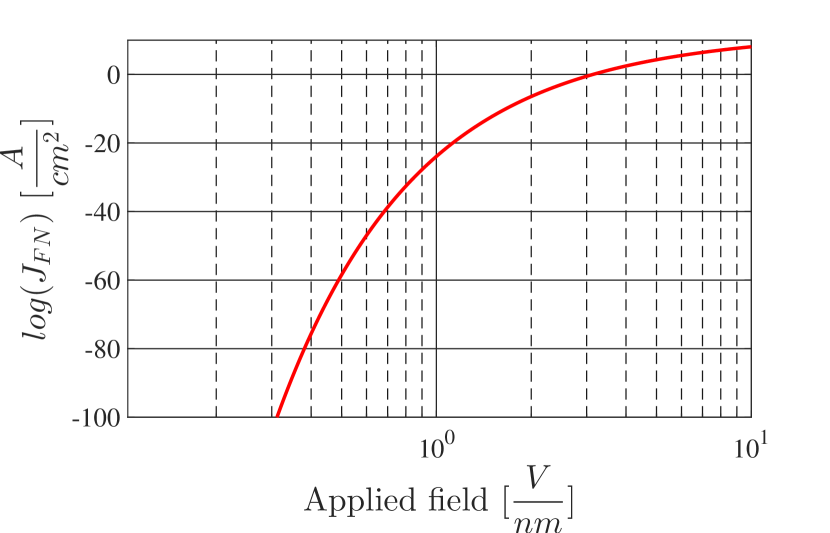
(a)

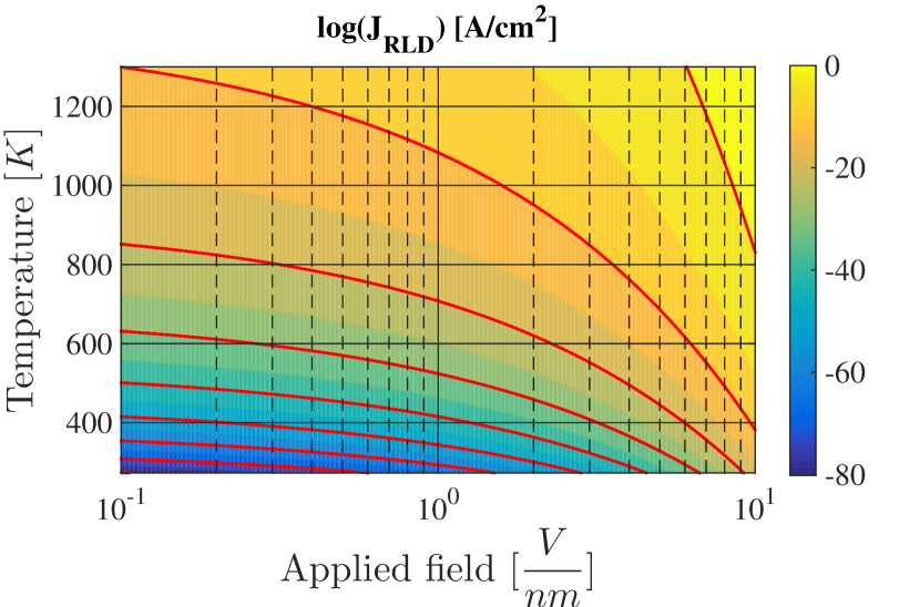
(b)

Figure 2: a) FN emission (temperature independent), b) thermal emission (red lines indicate isocurrent curves starting from 0 with steps of -10$\,\mathrm{A/cm^{2}}$). In both calculations, gold’s Fermi level of 5.53 eV and work function of 5.1 eV were used.

In calculations of tunneling probability through a barrier, it is common to define a Gamow factor, $\theta\left(\varepsilon\right),$ so that $T\left(\varepsilon\right)\propto e^{-\theta\left(\varepsilon\right)}.$ The Gamow factor carries the barrier shape information and is defined as (WKB formulation)

$$\theta\left(\varepsilon\right)=2\intop_{x_{-}}^{x_{+}}\sqrt{\frac{2m}{h^{2}}\left(V\left(x\right)-\varepsilon\right)}dx,$$ (12)

where $V\left(x_{\pm}\right)=\varepsilon.$ In fact, $\theta\left(\varepsilon\right)$ is defined as the area under the curve of the potential barrier ($V\left(x\right)$) between $x_{-}$ and $x_{+}$. A known example of defining $T\left(\varepsilon\right)$ based on the Gamow factor is given by $T\left(\varepsilon\right)=1/\left(1+e^{\theta\left(\varepsilon\right)}\right)$ Kemble (1935). There are two more parameters which are useful to review before moving to the next section. The value of $\varepsilon$ which maximizes the integrand in (5) is of special importance and is usually specified by $\varepsilon_{\mathrm{m}}.$ The field slope function, $\beta_{\mathrm{F}}$, and the slope factors ratio, n, are also defined as

$$\beta_{\mathrm{F}}=-\frac{\partial}{\partial\varepsilon}\theta\left(\varepsilon=\varepsilon_{\mathrm{m}}\right),$$ (13)

$$n=\beta_{\mathrm{T}}/\beta_{\mathrm{F}}.$$ (14)

It is also important to know the limitation of using (8) which is due to the zero temperature approximation of the supply function in finding the tunneling probability. This approximation is valid for low, including room, temperatures as the tunneling probability is dominated by the contribution of electrons around the chemical potential level.

So far we have reviewed thermal and field emissions separately. If the applied filed is negligible or the temperature is low, one can use (7) or (8), respectively. However, often these two physics are involved simultaneously which requires the use of the general thermal field (GTF) emission theory (readers can find detailed discussions about GTF in Jensen and Cahay (2006)). Based on GTF, we may consider three operating regimes for an electron emitter: thermal, field, and the transition regime where both thermal and field emissions become comparable.

In the next section, for engineering purposes and without going into equations derivings, we summarize the steps to estimate thermal/field electron emission when both the temperature and the applied filed are known.

III The general thermal-field emission model (with approximation)

Several parameters of electric field emission such as scattering rates and electrons distribution are temperature dependent. Besides, electrons departure due to the electric field emission may change the emitter’s temperature by extracting its energy. In fact, temperature is the key parameter which couples field and thermal emissions together in the general thermal-field emission theory. Details of this theory is discussed in Jensen and Cahay (2006); Jensen (2007), and is briefly summarized in the appendix. Here, we use a critical approximations which simplifies the formulation and provides an appropriate estimate of the thermal and field emitted electrons from metallic photocathodes. The approximation is based on the assumption that emitted electrons do not change the photocathode’s temperature. This is valid if either the photocathode’s operating temperature is low, or quantum yield (QY) of the photocathode is small. QY of a photocathode is the ratio of the emitted electrons to the penetrated photons (QY differs from QE by a factor of photon’s reflectivity from the photocathode’s surface). Despite the fact that metals reflectivity is very high, their QY is a small number because of their very small QE (less than 1%). To be more specific, the highest experimental QE of metals is about 0.22% and is produced by a laser excitation of 0.6$\,\mathrm{mJ/cm^{2}}$ and under a 50$\,\mathrm{MV/m}$ static field. Assuming gold as the photocathode (with the permittivity of $\varepsilon_{\mathrm{r}}=-22-1.5i$ at 785 nm), the reflection coefficient of an IR wave is around 98.62% at normal incidence. Simple calculation shows that about 15% of penetrated photons are contributing to direct electron emission. We simply disregard the cooling effect of these emitted electrons and assume that penetrated photons are entirely absorbed by phonons in the metal, leading to a temperature rise. Note that 0.6$\,\mathrm{mJ/cm^{2}}$ laser intensity is very high, and QE of usual photocathodes is considerably smaller than 0.22%. Nonetheless, there is always the choice of referring to the appendix to perform more accurate and more complex calculations.

In this low QY regime, total field-thermal emission contributions of a photocathode (or any emitter) can be obtained using the following steps (with the aid of commercially available electromagnetic solvers):

1) The first step is to obtain the photocathode’s approximate temperature using electromagnetic and heat transfer calculations. The assumption here is that electron and lattice temperatures are equal, and electron emission does not affect the temperature. A simple method is to perform a full-wave electromagnetic simulation and find the absorbed laser power by the photocathode. Then, the absorbed laser power can be considered as the heat source in the heat transfer calculations. This can be done analytically, or by a simulation solver along with the appropriate convection, conduction, or radiation boundaries. Either of the calculations should provide us the temperature distribution on the photocathode. If the computational power allows us, a better approach is to perform a coupled electromagnetic and heat transfer simulation (e.g. using Multiphysics simulation is COMSOL). As a check point, from the maximum temperature on the photocathode, we may validate the approximation (i.e., to confirm the temperature is not too high, e.g. >1000 K). We may consider the maximum calculated temperature in the structure as the operating temperature, $T_{\mathrm{o}}.$ Note that the maximum temperature obtained by this method is always larger than the actual temperature since a fraction of the absorbed photons contribute to direct photoemission.

2) The second step is to determine the dominant operating regime of the photocathode, which can be thermal, field, or the transition regime (where thermal and field contributions are comparable). After finding Shottkey reduced work function ($\phi$), and Fowler parameter ($y$), thermal coefficients

$$B_{\mathrm{q}}=\frac{\pi}{\hbar}\phi\sqrt{2m}\left(\frac{Q}{F_{\mathrm{static}}^{3}}\right)^{1/4};\qquad C_{\mathrm{q}}=-\frac{B_{\mathrm{q}}}{\phi},$$ (15)

and Fowler-Nordheim coefficients

$$C_{\mathrm{FN}}=-\frac{2}{\hbar F}\sqrt{2m\Phi}t\left(y\right);\qquad B_{\mathrm{FN}}=\frac{4}{3\hbar F}\sqrt{2m\Phi^{3}}v\left(y\right),$$ (16)

$$C_{\mathrm{n}}=-\frac{3B_{\mathrm{FN}}+\left(2C_{\mathrm{FN}}+C_{\mathrm{q}}\right)\phi}{\phi^{2}};\qquad D_{\mathrm{n}}=\frac{2B_{\mathrm{FN}}+\left(C_{\mathrm{FN}}+C_{\mathrm{q}}\right)\phi}{\phi^{3}}$$ (17)

should be found, in which Forbes approximation are applicable to find $v$ and $t$ as given by (9) and (10). Then, the two threshold temperatures $T_{\mathrm{min}}$ and $T_{\mathrm{max}}$

$$T_{\mathrm{min}}=-\frac{1}{k_{\mathrm{B}}C_{\mathrm{FN}}};\qquad T_{\mathrm{max}}=-\frac{1}{k_{\mathrm{B}}C_{\mathrm{q}}}$$ (18)

determine the operating regime of the photocathode. Thermal and field regimes are identified by $T_{\mathrm{o}}>T_{\mathrm{max}}$ and $T_{\mathrm{o}}<T_{\mathrm{min}}$, respectively. The transition regime is identified by $T_{\mathrm{min}}<T_{\mathrm{o}}<T_{\mathrm{max}}.$ Detailed explanations regarding these regimes and how the formulations are derived are explained in Jensen (2007).

4) The total current due to the thermal-field emission can be obtained from Jensen (2017)

$$J_{\mathrm{GTF}}=A_{\mathrm{RLD}}\left(k_{\mathrm{B}}\beta_{\mathrm{T}}\right)^{-2}N\left(n,s\right),$$ (19)

$$N\left(n,s\right)=s_{\mathrm{ng}}+s_{\mathrm{n}}e^{\mathrm{-ns}}+n^{2}s_{\mathrm{d}}e^{\mathrm{-s}}.$$ (20)

$$s_{\mathrm{d}}=-n^{-2}\left(0.10593434n^{-2}+0.35506593\right)-1,$$ (21)

$$s_{\mathrm{n}}=-n^{2}\left(0.10593434n^{2}+0.35506593\right)-1,$$ (22)

$$s_{\mathrm{ng}}=\begin{cases}\begin{array}[]{c}-2\left[e^{\mathrm{-ns}}-n^{4}e^{\mathrm{-s}}\right]\left[n^{2}-1\right]^{-1}\\ e^{\mathrm{-s}}\left[24s^{3}\left(s+4\right)-z^{3}\left(s^{4}-24\right)+4sz^{2}\left(s^{3}+24\right)-12s^{2}z\left(s^{2}-12\right)\right]\left[12s^{2}\left(2s+z\right)\right]^{-1}\end{array}&\begin{array}[]{c}\left|z\right|>0.1\\ \left|z\right|<0.1\end{array},\end{cases}$$ (23)

where $z=s\left(n-1\right),$ and parameters n and s depend on the operating regime (identified by $T_{\mathrm{o}}$), and are given in Table I.

Table 1: s and n for different operating regimes.

	s	n
Thermal $\left(n<1\right)$	$B_{\mathrm{q}}$	$\phi\beta_{\mathrm{T}}/B_{\mathrm{q}}$
Field $\left(n>1\right)$	$B_{\mathrm{FN}}$	$-\beta_{\mathrm{T}}/C_{\mathrm{FN}}$
Transition $n=1$	Eq. ((24))	$1$

In Table I, for the transition regime $\left(n=1\right)$,

$$s=B_{\mathrm{FN}}-C_{\mathrm{n}}\left(\varepsilon_{\mathrm{m}}-\mu\right)^{2}-2D_{\mathrm{n}}\left(\varepsilon_{\mathrm{m}}-\mu\right)^{3},$$ (24)

$$\varepsilon_{\mathrm{m}}=\mu-\frac{C_{\mathrm{n}}}{3D_{\mathrm{n}}}+0.5\sqrt{\left(\frac{2C_{\mathrm{n}}}{3D_{\mathrm{n}}}\right)^{2}-4\frac{\beta_{\mathrm{T}}+C_{\mathrm{FN}}}{3D_{\mathrm{n}}}}.$$ (25)

Before adding the photo-emitted contribution, it is useful to compare different regimes as a function of the applied static field and the temperature. Figure 3 shows $J_{\mathrm{GTF}}$ of a gold cathode. By comparing $J_{\mathrm{GTF}}$, $J_{\mathrm{FN}}$, and $J_{\mathrm{RLD}}$ in Fig. 3(b), we can distinguish different operating regimes. The transition regime is where $0.5\mathrm{\frac{V}{nm}}<F_{\mathrm{static}}<2\mathrm{\frac{V}{nm}}$.

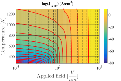
(a)

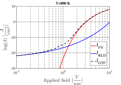
(b)

Figure 3: a) $J_{\mathrm{GTF}}$ as a function of the temperature and the applied field (red lines indicate isocurrent curves starting from 5$\,\mathrm{A/cm^{2}}$ with steps of -5$\,\mathrm{A/cm^{2}}$), b) comparison among $J_{\mathrm{FN}}$, $J_{\mathrm{RLD}}$, and $J_{\mathrm{GTF}}$ at T=800 K. In all calculations, gold’s Fermi level of 5.53 eV and work function of 5.1 eV were used.

IV Photoemission by short wavelength lasers

One of the most known models of photoemission is the three step model of Spicer and Perrera-Gomez, developed in 1958 (a review of this model is given in the appendix) Spicer and Herrera-Gomez (1993). The three steps in this model are a) optical absorption by the material, b) electron transport inside the material, and c) electron emission (escape) from the material surface. These three steps can be seen in Fowler-Dubridge equation as

$$J_{\mathrm{\lambda}}=I_{\mathrm{\lambda}}\left(\frac{q}{\hbar\omega}\right)\left(1-R\right)f_{\mathrm{\lambda}}P,$$ (26)

in which R is the reflection from the photocathode surface, $f_{\mathrm{\lambda}}$ is the probability of an excited electron to reach the surface without experiencing any collision, and P is the probability of emission from the metal surface.

Having proper electromagnetic model of the photocathode’s material (e.g. permittivity model), it is fairly easy to calculate the photocathode reflectivity (which leads to the photon absorption). In a one dimensional geometry with normal laser incidence, reflectivity can be found from

$$R=\left|\frac{1-\sqrt{\epsilon_{\mathrm{r}}}}{1+\sqrt{\epsilon_{\mathrm{r}}}}\right|,$$ (27)

where $\epsilon_{\mathrm{r}}$ is the relative permittivity of the metal at $\lambda.$ A more general equation for the reflectivity under oblique incidence is given in the appendix. For complex geometries, numerical Maxwell equation solvers can easily calculate the reflectivity or the absorption of the photocathode.

The second step is electrons travel to the surface, which usually initiates by an applied static field drifting electrons to the surface. On their path, these electrons experience electron-electron and electron-phonon scatterings, as well as change of momentum directions. In most photoemission models, the assumption is that a single collision extracts most of the electron’s energy and prevents it from contributing to direct photoemission. Often, the scattering rate is replaced by the mean free path of an electron, which is the collision-free travel range of an electron in the metal. In metals, electron-electron scattering is dominant and electrons mean free path can be obtained from Dowell et al. (2006)

$$\lambda_{\mathrm{e-e}}=\frac{2\lambda_{\mathrm{m}}\varepsilon_{\mathrm{m}}^{3/2}}{\hbar\omega\sqrt{\phi}\left(1+\sqrt{\frac{\phi}{\hbar\omega}}\right)},$$ (28)

where $\lambda_{\mathrm{m}}$ and $\varepsilon_{\mathrm{m}}$ are experimentally measured energy and mean free path values which are available in Dowell et al. (2006). $\delta$ is the skin depth which depends on the imaginary part of the permittivity, $k$, as $\delta=\frac{\lambda}{4\pi k}$. Then,

$$f_{\mathrm{\lambda}}=\intop_{0}^{\infty}\frac{1}{\delta}e^{-x\left(1/\delta+1/\lambda_{\mathrm{e-e}}\right)}dx=\left(1+\frac{\delta\left(\omega\right)}{\lambda_{\mathrm{e-e}}\left(\omega\right)}\right)^{-1}$$ (29)

A more accurate equation for $f_{\mathrm{\lambda}}$ is to use (67) in the appendix, however a good approximation, which we will use throughout this paper is

$$f_{\mathrm{\lambda}}=0.5G\left(\frac{\delta m}{\hbar k_{\mathrm{v}}\tau}\right),$$ (30)

$$G\left(x\right)=\left\{\begin{array}[]{cc}1-\frac{2cos^{-1}\left(1/x\right)}{\pi sin\left(cos^{-1}\left(1/x\right)\right)}&x>1\\ 1-\frac{1}{\pi}cot\left(cos^{-1}\left(x\right)\right)ln\left[\frac{1+sin\left(cos^{-1}\left(x\right)\right)}{1-sin\left(cos^{-1}\left(x\right)\right)}\right]&x<1\end{array},\right.$$ (31)

tin which $\hbar k_{\mathrm{v}}=\sqrt{2m\left(\mu+\phi\right)}$, $\tau$ is the scattering rate (its value for gold at 537 K is 11.85 fs), and $\delta$ is the skin depth.

The third step is the emission of electrons from the metal surface. The important effects in this step are Schottky effect, the abrupt change in the electron angle across the metal-vacuum transition, and the scattering (reflection) from the surface. In many models including Fowler-Dubridge model, quantum effects such as tunneling and multiphoton absorption are neglected, and only electron transport over the potential barrier is considered. This is sometimes called the thermionic approximation, and it should not be confused with the emission due to the thermal effect. Based on Fowler-Dubridge mode, excited electrons can emit only if their energy is higher than the work function. Therefore, the probability of electron emission at the surface is

$$P=\frac{\intop_{\mu+\phi-\hbar\omega}^{\infty}f\left(E\right)dE}{\intop_{0}^{\infty}f\left(E\right)dE}.$$ (32)

Considering Fermi-Dirac distribution for electrons leads to

$$P=\frac{U\left[\frac{1}{k_{\mathrm{B}}T}\left(\hbar\omega-\phi\right)\right]}{U\left(\frac{1}{k_{\mathrm{B}}T}\mu\right)},$$ (33)

where $U$ is the Fowler function defined as

$$U\left(x\right)=\intop_{-\infty}^{\mathrm{x}}ln\left(1+e^{\mathrm{y}}\right)dy.$$ (34)

There are several approximations for (34) such as Jensen et al. (2005)

$$U\left(x\right)=\begin{cases}\begin{array}[]{c}e^{\mathrm{x}}\left(1-0.17753e^{0.72843x}\right)\\ \frac{x^{2}}{2}+\frac{\pi^{2}}{6}-e^{\mathrm{-x}}\left(1-0.17753e^{\mathrm{-0.72843x}}\right)\end{array}&\begin{array}[]{c}x<0\\ x\geqslant 0\end{array}\end{cases}.$$ (35)

There are also several approximations reported for (33) such as the simple approximation Dowell et al. (2006)

$$P=\frac{\left(\mu+\hbar\omega\right)}{2\hbar\omega}\left[1+\frac{\mu+\phi}{\mu+\hbar\omega}-2\sqrt{\frac{\mu+\phi}{\mu+\hbar\omega}}\right],$$ (36)

and the more accurate equation Jensen et al. (2007)

$$P=\left\{\frac{3\left(\hbar\omega-\phi\right)^{2}+\beta^{2}\pi^{2}\left[1+n^{2}\right]}{6\hbar\omega\left(2\mu-\hbar\omega\right)}\right\},$$ (37)

in which

$$n=\frac{1}{\pi k_{\mathrm{B}}T}\sqrt{\frac{\hbar^{2}}{2m}}\left(\frac{F_{\mathrm{static}}^{3}}{Q}\right)^{1/4}.$$ (38)

A crucial point in all of these equations is the assumption that $\hbar\omega$ is larger than $\phi$, which is true in most photocathode designs (e.g. UV photocathodes). However, (33) does not apply to long wavelength photocathodes (e.g. IR) where there are potential applications as discussed in the introduction.

Note that $J_{\mathrm{\lambda}}$ is the emission by direct photo-excitation, and is different from the emission stimulated by the laser heating. For example, as calculated in Jensen et al. (2006), for a laser intensity of 28$\,\mathrm{MW/cm^{2}}$ with a Gaussian pulse with 2.7 ns time constant and a wavelength of 800 nm, along with a static field of 8$\,\mathrm{MV/m}$ at room temperature, the thermal illumination-induced current is 3.8% of the total photoemission current for a coated tungsten surface with work function of 1.9 eV.

V Photoemission by long wavelength lasers

The three step model (i.e. using (26)) applies to photoemission by long wavelength lasers as well. However, since excited electrons do not have enough energy to overpass the barrier, (32) needs to be generalized to include tunneling through the barrier. In general, P as the emission probability of an electron (consecutive to a photon absorption) at the photocathode’s surface can be written as

$$P=\frac{\intop_{0}^{\infty}T\left(\varepsilon+\hbar\omega\right)f\left(\varepsilon\right)d\varepsilon}{\intop_{0}^{\infty}f\left(\varepsilon\right)d\varepsilon}.$$ (39)

Equation (39) can be decomposed into the transmission over the barrier (i.e. $E+\hbar\omega>\mu+\phi$) and tunneling through the barrier as

$$P=P_{\mathrm{over}}+P_{\mathrm{tunnel}},$$ (40)

$$P_{\mathrm{over}}=\frac{\intop_{\mu+\phi-\hbar\omega}^{\infty}T\left(\varepsilon+\hbar\omega\right)f\left(\varepsilon\right)d\varepsilon}{\intop_{0}^{\infty}f\left(\varepsilon\right)d\varepsilon}$$ (41)

$$P_{\mathrm{tunnel}}=\frac{\intop_{0}^{\mu+\phi-\hbar\omega}T\left(\varepsilon+\hbar\omega\right)f\left(\varepsilon\right)d\varepsilon}{\intop_{0}^{\infty}f\left(\varepsilon\right)d\varepsilon}.$$ (42)

An acceptable approximation for (41) is to use the step function as $T\left(E+\hbar\omega\right)$, as in Fowler-Dubridge model, which leads to (32) and (33). More accurate expressions can be found quantum mechanically which provides a negligible improvement.

For electrons with energies such that $E+\hbar\omega<\mu+\phi$, the transmission function can be found using the Gamow factor technique. However, similar to Fowler-Nordheim formulation, we may use zero temperature approximation for $f\left(E\right)$ and adjust the upper integral limit as $\left(\mu+\phi-\hbar\omega\right)\rightarrow\mu$ (because there is no electron above $\mu,$ and electrons near $\mu$ have the highest probability of tunneling). Then, considering the numerator of (42) and (4), it is straightforward to show that

$$\intop_{0}^{\mathrm{\mu}}T\left(\varepsilon+\hbar\omega\right)f\left(\varepsilon\right)d\varepsilon=\frac{2\pi\hbar}{q}J_{\mathrm{FN}}\left(\Phi\rightarrow\Phi-\hbar\omega\right)$$ (43)

in which $J_{\mathrm{FN}}\left(\Phi\rightarrow\Phi-\hbar\omega\right)$ is (8) after the replacement $\Phi\rightarrow\Phi-\hbar\omega.$ Therefore, the final expression for $P$ is

$$P=\frac{\intop_{\mu+\phi-\hbar\omega}^{\infty}f\left(\varepsilon\right)d\varepsilon+\frac{2\pi\hbar}{q}J_{\mathrm{FN}}\left(\Phi\rightarrow\Phi-\hbar\omega\right)}{\intop_{0}^{\infty}f\left(\varepsilon\right)d\varepsilon}$$ (44)

Equation (44) can be organized as

$$P=\frac{U\left[\beta_{\mathrm{T}}\left(\hbar\omega-\phi\right)\right]}{U\left(\beta_{\mathrm{T}}\mu\right)}\Theta\left(\hbar\omega-\phi\right)+\frac{\pi\hbar^{2}\beta_{\mathrm{T}}^{2}F_{\mathrm{static}}^{2}}{qm\left(\Phi-\hbar\omega\right)4t^{2}U\left(\beta_{\mathrm{T}}\mu\right)}exp\left[\frac{-\nu 8\pi\sqrt{2m}\left(\Phi-\hbar\omega\right)^{1.5}}{3hF}\right],$$ (45)

where $\Theta$ is the Heaviside step function, and indicates that the first term should be applied only if $\hbar\omega>\phi.$ Equation (45), as the generalized photoemission probability, enables us to estimate the photoemission contribution when the illuminating laser has a photon energy lower than the lowered work function of the cathode. Figure 4(a) shows (44) as a function of the applied field for a gold photocathode at $\lambda=785\,nm$ and T=273 K. The photoemitted current, $J_{\mathrm{\lambda}}$, as a function of the laser wavelength and the applied field is shown in Figure 4(b). The laser intensity is assumed to be 5$\,\mathrm{W/cm^{2}}$.

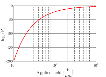
(a)

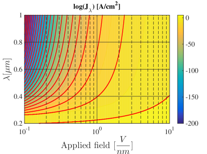
(b)

Figure 4: a) Equation (44) as a function of the temperature and the applied field, b) $J_{\mathrm{\lambda}}$ at T=273 K (red lines indicate isocurrent curves starting from 0 with the separation of -10$\,\mathrm{A/cm^{2}}$)). In all calculations, gold’s Fermi level of 5.53 eV and work function of 5.1 eV were used.

VI Photoemission by resonant photocathodes

If resonance effect is included in the photocathode design, it can impact/improve all three steps of the photoemission process. An example of such photocathodes are metallic IR photocathodes with plasmonic resonant field enhancement Putnam et al. (2017). It is common to approach resonant effects with their quality factor, Q. However, for our purpose, it is more conveient to consider their equivalent electric field enhancement factor which is defined as the ratio of the electric field on the cavity surface ($F_{\mathrm{cavity}}$) to the incident electric field $\left(F_{\mathrm{laser}}\right)$

$$\alpha_{\mathrm{enhance}}=\frac{F_{\mathrm{cavity}}}{F_{\mathrm{laser}}}=\frac{F_{\mathrm{cavity}}}{q\sqrt{240\pi I_{\mathrm{\lambda}}}}.$$ (46)

Note that $F_{\mathrm{cavity}}$ for metals is normal to the cavity surface, and it’s value can be related to Q as discussed in Li et al. (2017, 2016). Typical values of $\alpha_{\mathrm{enhance}}$ are in the range $10\sim 100$ for noble metals at IR wavelengths. Since the electric field on the cavity surface is enhanced by $\alpha_{\mathrm{enhance}}$, it is a good approximation to assume that penetrated photons inside the cavity are enhanced by a factor of $\alpha_{\mathrm{enhance}}^{2}$. The resonance effect also changes the scattering rate inside the cavity, and the assumptions for obtaining (30) is no longer valid (e.g. there is not a plane wave traveling inside the metal anymore). However, extracting a new $f_{\mathrm{\lambda}}$ for different cavity shapes is beyond the scope of this paper, and we keep using (30) as an approximation. Moreover, if $\alpha_{\mathrm{enhance}}F_{\mathrm{laser}}$ becomes comparable with the applied static field, it can contribute in the barrier reduction and the replacement $F\rightarrow\left(F_{\mathrm{static}}+F_{\mathrm{cavity}}\right)$ should be made in (2) leading to

$$\phi_{\mathrm{cavity}}==\Phi-\sqrt{4Q\left(F_{\mathrm{static}}+\alpha_{\mathrm{enhance}}q\sqrt{240\pi I_{\mathrm{\lambda}}}\right)},$$ (47)

where $F_{\mathrm{static}}$ is the applied static field to the photocathode. The final photoemission equation is then

$$J_{\mathrm{\lambda}}=I_{\mathrm{\lambda}}\left(\frac{q}{\hbar\omega}\right)\alpha_{\mathrm{enhance}}^{2}f_{\mathrm{\lambda}}P_{\mathrm{cavity}},$$ (48)

where

$$P_{\mathrm{cavity}}=\frac{U\left[\beta_{\mathrm{T}}\left(\hbar\omega-\phi_{\mathrm{cavity}}\right)\right]}{U\left(\beta_{\mathrm{T}}\mu\right)}\Theta\left(\hbar\omega-\phi_{\mathrm{cavity}}\right)+$$

$$\qquad\qquad\frac{\beta_{\mathrm{T}}}{U\left(\beta_{\mathrm{T}}\mu\right)}\frac{\left(F_{\mathrm{static}}+\alpha_{\mathrm{enhance}}q\sqrt{240\pi I_{\mathrm{\lambda}}}\right)^{2}}{\left(\Phi-\hbar\omega\right)8\pi t^{2}}exp\left[\frac{-\nu 8\pi\sqrt{2m}\left(\Phi-\hbar\omega\right)^{1.5}}{3h\left(F_{\mathrm{static}}+\alpha_{\mathrm{enhance}}q\sqrt{240\pi I_{\mathrm{\lambda}}}\right)}\right],$$ (49)

At last, adding the thermal-field emission to the photoemission gives the total current of the photocathode as

$$J=J_{\mathrm{GTF}}+J_{\mathrm{\lambda}}.$$ (50)

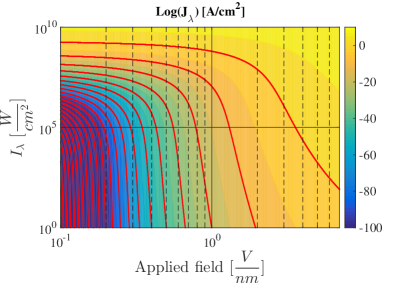
(a)

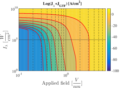
(b)

Figure 5: a) $J_{\mathrm{\lambda}}$ and b) $J_{\mathrm{\lambda}}+J_{\mathrm{GTF}}$ of a resonant photocathode with $\alpha_{\mathrm{enhance}}=20$ at T=273 K (red lines indicate isocurrent curves starting from 0 with the separation of -10$\,\mathrm{A/cm^{2}}$)). In all calculations, gold’s Fermi level of 5.53 eV and work function of 5.1 eV were used.

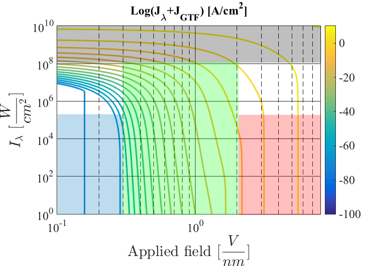
Figure 6: Different emission regions of the total current (explanation in the text). Parameters are the same as Fig. 5.

Figure 5 shows the photo-emitted current component, $J_{\mathrm{\lambda}}$, and the total current, $J_{\mathrm{\lambda}}+J_{\mathrm{GTF}}$, as a function of the irradiance power and the applied field. The optical enhancement factor of 20 is assumed for the photocathode, the wavelength is fixed at 785 nm, and gold parameters are used for the photocathode. Four important regions of the total current are specified in Fig. 6. The blue region is where both field emission and photoemission currents are negligible, and only thermal emission at 273 K (a small number) exists. In the red region, field emission is dominant and changing the laser intensity does not have much effect on the total current. Inversely, in the gray region, photoemission current dominates the total current and the applied static field does not have a comparable effect. The green region is where both field emission and photoemission are comparable, and is useful for designing microelectronic devices with both voltage and optical controls. This region is identified by $0.2<F_{\mathrm{static}}[\mathrm{\frac{V}{nm}}]<2$ and $I_{\mathrm{\lambda}}<100\,\mathrm{\frac{MW}{cm^{2}}}$ for gold photocathode at $\lambda=785\,$nm, and can be obtained for different materials in a similar fashion. As the final note on this section, a very useful list of experimental parameters for different metals are given in Table I of Jensen et al. (2006).

(a)

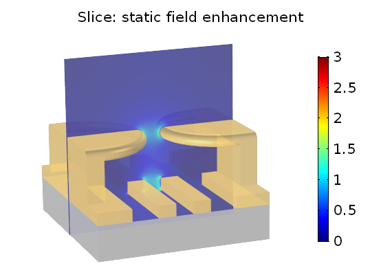
(b)

Figure 7: a) unit cell of the resonant photocathode (array of 12 by 12 elements), b) simulated static electric field enhancement of the photocathode. The smallest gap size is 100 nm, and the metal is gold (see Forati et al. (2016); Forati and Sievenpiper (2016)).

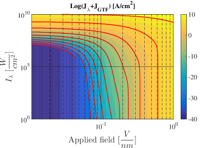
Figure 8: Total current ($J_{\mathrm{\lambda}}+J_{\mathrm{GTF}}$) of the photocathode at T=550 K with the optical and static enhancement factors of 37.2 and 9, respectively. Red lines indicate isocurrent curves starting from 10 with steps of -5$\,\mathrm{A/cm^{2}}$. Gold’s Fermi level of 5.53 eV and work function of 5.1 eV were used.

VII Example

Figure 7(a) shows the unit cell of the IR photocathode studied in Forati et al. (2016), experimentally. The photocathode is fabricated using gold on Si substrate with a $200\,$nm $SiO_{2}$ in between as isolation. The surface area of the photocathode is around 450 $\mu\,$m (22 by 22 unit cells with the area of about 1 by 1 micron), and the minimum gap size is $100\,$nm. As reported in Forati et al. (2016), full wave simulated (using COMSOL) and measured optical electric field enhancement of the photocathode were 12 and 37, respectively. The factor of 3 difference was due to the surface roughness of the fabricated device, which was not considered in the simulations. Solving Poisson’s equation on the same unit cell in COMSOL leads to the static electric field enhancement of $2.5\sim 3$, as Fig. 7(b) shows. Using the additional factor of 3 due the surface roughness, we perform our calculations with the static electric filed enhancement of 9. Figure 8 shows the total current emission of the photocathode as a function of the applied static field and the laser intensity. The wavelength is 875 nm, the temperature is assumed to be 550 K (which seems to be a reasonable guess). Complex permittivity values of $\epsilon_{\mathrm{Si}}=13.734-0.054952i$ and $\epsilon_{\mathrm{SiO_{2}}}=2.1502-0i$ were used for silicon and $SiO_{2},$ respectively https://refractiveindex.info/?shelf=main&book=SiO2&page=Lemarchand .

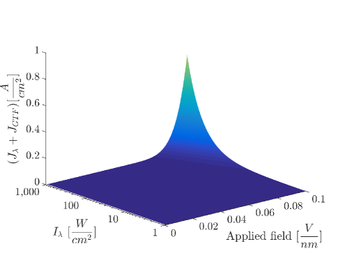
Figure 9: Total current ($J_{\mathrm{\lambda}}+J_{\mathrm{GTF}}$) of the resonant photocathode at T=550 K with the optical and static enhancement factors of 300 and 10, respectively. Gold’s Fermi level of 5.53 eV and work function of 5.1 eV were used.

Comparing the the experimental values reported in Forati et al. (2016) with Fig. 8, either a higher field enhancement factor (for the static or the laser field) should be considered, or the thermal effect is considerable. Note that our suggested theory for long wavelength photoemission, including (49), was based on a low temperature assumption. The approximations in our formulations may not be valid if the laser intensity can change the photocathode temperature considerably. With the available experimental data reported in Forati et al. (2016), we cannot confirm if the temperature of the photocathode rises significantly. But, plasmoinc resonance effects are claimed to be capable of providing laser field enhancements on the order of 1000 Ward et al. (2010). An important conclusion can be made if draw Fig. 8 on a linear scale, as shown in Fig. 9 (note that field enhancements are changed to 10 and 1000 for the static and laser fields, respectively). Figure 8 shows that, above a certain threshold, simultaneous application of both laser and static fields can cause significant electron emission. In contrast, neither static nor optical field alone generates nearly as much current as both fields combined. This result is also consistent with the results in Piltan and Sievenpiper (2017) which are based on the analytical solution for Schrodinger equation with a triangular work function Zhang and Lau (2016). The analytical solution in Zhang and Lau (2016) is general and considers the multiphoton absorption/emission effect. However, the results in this paper are only based on single photon absorption, hence their accuracy becomes questionable at strong laser fields (intensities above 1e10 ${\mathrm{(W/cm^{2}}}$). Note that the results in Zhang and Lau (2016) unnecessarily disregards the charge image effect (Schottkey effect) in most of the generated results (which is significant for the applied static field range). Moreover, the solution in Zhang and Lau (2016) only assumes electrons at the Fermi level while the results in this paper includes the supply function of the metal.

VIII Conclusion

Electron emission theories were reviewed and a formulation was extracted for the electron emission by photocathodes under exposure of long wavelength lasers. With the summarized formulations in this paper, an optimal range for the applied static field and laser illumination was obtained for gold photocathodes so that both $J_{\mathrm{\lambda}}$ and $J_{\mathrm{F}}$ are comparable. This condition is needed for the design of nano-electronic devices with both optical and voltage controls. The effect of optical resonance was also shown to be significant in the performance of photocathodes. This can include generation of electron beams with strong correlation with the incoming photons.

IX Acknowledgement

The authors would like to thank Dr. Kevin Jensen for his generous help to better understand his theories and results.

X Appendix

X.1 The three step model of Spicer and Perrera-Gomez Spicer and Herrera-Gomez (1993)

The three steps of the model are a) optical absorption by the material, b) electron transport inside the material, and c) electron emission (escape) from the material surface. The laser intensity inside the material can be written as

$$S\left(x,\lambda\right)=S_{0}\left(1-R\right)e^{-\alpha x}$$ (51)

where $S_{0}$ is the incident laser intensity, $R$ is the reflection from the material surface which depends on the wavelength, $\alpha$ is the laser attenuation inside the material both due to absorption by electrons and phonons, and $x$ is the 1D coordinate with the material boundary at $x=0$. Note that both $R$ and $\alpha$ are wavelength dependent.

The light absorption is the rate of the light intensity decrease as

$$dS\left(x,\lambda\right)=\alpha S_{0}\left(1-R\right)e^{\mathrm{-\alpha x}}dx.$$ (52)

Consider a slab between $x$ and $x+dx$. Only a portion of the absorbed photons in this slab can lead to electron liberation from the material surface. The contribution of these photons into the emitted current can be written as

$$di\left(x\right)=P_{o\alpha}\left(\lambda,x,dx\right)P_{\mathrm{T}}\left(\lambda,x\right)P_{\mathrm{E}}\left(\lambda\right)$$ (53)

where $P_{o\alpha}$ is the probability of exciting electrons above the vacuum level (VL) by photons absorbed in the slab between x and x+dx, $P_{\mathrm{T}}$ is the probability that electrons will reach the surface without losing their sufficient energy, and $P_{\mathrm{E}}$ is the probability of escape from the surface. Let us define $\alpha_{\mathrm{PE}}$ as the probability of exciting an electron above the VL by a photon so that

$$P_{o\alpha}\left(x,dx\right)=\alpha_{\mathrm{PE}}I_{x}dx=\alpha_{\mathrm{PE}}I_{0}\left(1-R\right)e^{\mathrm{-\alpha x}}dx,$$ (54)

and define the escape length, $L$, so that

$$P_{\mathrm{T}}=exp\left(-\frac{x}{L}\right).$$ (55)

Then, (53) can be written as

$$di\left(x\right)=\alpha_{\mathrm{PE}}I_{0}\left(1-R\right)e^{\mathrm{-\alpha x}}e^{\mathrm{-x/L}}P_{\mathrm{E}}dx.$$ (56)

This gives us QE as

$$QE=\frac{1}{I_{0}}\intop_{0}^{\infty}di\left(x\right)dx=\left(1-R\right)e^{\mathrm{-\alpha x}}\frac{\alpha_{\mathrm{PE}}P_{\mathrm{E}}}{\alpha+1/L}.$$ (57)

It is usual to define an absorption length as $l_{\mathrm{\alpha}}=1/\alpha$ and re-write 57 as

$$QE=\left(1-R\right)e^{\mathrm{-\alpha x}}\frac{\frac{\alpha_{\mathrm{PE}}}{\alpha}P_{\mathrm{E}}}{1+l_{\mathrm{\alpha}}/L}.$$ (58)

Parameters $L,$ $P_{\mathrm{E}},$ and $\alpha_{\mathrm{PE}}$ are measured experimentally and reported for different photocathodes. Also, from Maxwell’s equations, $R$ and $\alpha$ can be calculated knowing the permittivity of the photocathode material.

The ratio $\alpha_{\mathrm{PE}}/\alpha$ is the fraction of electrons excited above the VL. This ratio is maximized by lowering the vacuum level to be close to the conduction band minimum (CBM). This ratio for effective emitters is usually between 0.1 and 1. Emitters with negative electron affinity have this ratio at around unity. The negative affinity cathodes were the first “significantly engineered” photocathodes introduced in 1965. The parameter $\alpha_{\mathrm{PE}}$ usually increases with the photon energy.

By examining the ratio $l_{\mathrm{a}}/L$, it is clear that faster absorption of the light leads to a higher QE. In other words, high energy photons are disadvantageous in this regard since they can travel far into the metal. The parameter $P_{\mathrm{E}}$ is usually less than 0.1 for metals, and it usually increases monolithically with the incident photon energy.

X.2 The general field-thermal model with temperature coupling (short wavelength)

This section is a summary of the model presented in Jensen (2007), which is the most comprehensive field-thermal emission model so far. This model calculates the electron and lattice temperatures using coupled differential equations which relates temperature to the laser power. Then, using thermal conductivity and optical parameters of materials, scattering and reflection of electrons and photons are calculated. The key point in this model is to find temperatures of electrons and lattice due to laser illumination. The following steps should be considered based on this model:

1) Find the absorbed laser power from

$$G\left(z,t\right)=I_{\mathrm{\lambda}}\left(t\right)\left(1-R\right)\frac{e^{\mathrm{-z/\delta}}}{\delta}\left\{1-P\left(\hbar\omega\right)\right\}$$ (59)

in which $R$ is the reflection from the material and $\delta=\frac{\lambda}{4\pi k}$ is the skin depth (note that $n+ik$ is known for the emitter material). For a two dimensional material, this parameter can be extracted from Snell’s law (for parallel and transverse polarizations), leading to

$$R=0.5\left(R_{\mathrm{s}}+R_{\mathrm{p}}\right),$$ (60)

$$R_{\mathrm{s}}=\frac{a^{2}+b^{2}-2acos\theta+cos^{2}\theta}{a^{2}+b^{2}+2acos\theta+cos^{2}\theta},$$ (61)

$$R_{\mathrm{p}}=R_{\mathrm{s}}\frac{a^{2}+b^{2}-2asin\theta tan\theta+sin^{2}\theta tan^{2}\theta}{a^{2}+b^{2}+2asin\theta tan\theta+sin^{2}\theta tan^{2}\theta},$$ (62)

$$2a^{2}=\left[\left(n^{2}-k^{2}-sin^{2}\theta\right)^{2}+\left(2nk\right)^{2}\right]^{0.5}+\left(n^{2}-k^{2}-sin^{2}\theta\right),$$ (63)

$$2b^{2}=\left[\left(n^{2}-k^{2}-sin^{2}\theta\right)^{2}+\left(2nk\right)^{2}\right]^{0.5}-\left(n^{2}-k^{2}-sin^{2}\theta\right).$$ (64)

$\theta$ is the incidence angle.

2) Find electron and lattice specific heat parameters as

$$C_{\mathrm{e}}\left(T_{\mathrm{e}}\right)=\frac{\gamma T_{\mathrm{e}}}{1+7/40\left(\pi/\beta_{\mathrm{e}}\mu\right)^{2}}$$ (65)

$$C_{\mathrm{i}}\left(T_{\mathrm{i}}\right)=\frac{3Nk_{\mathrm{B}}}{1+1/20\left(T_{\mathrm{D}}/T_{\mathrm{i}}\right)^{2}}$$ (66)

where $\beta_{\mathrm{e}}=1/k_{\mathrm{B}}T_{\mathrm{e}}$, and $N\left(\#/cm^{3}\right)$ is the number density of the crystal. Deby temperature and $\gamma$ are given in table I of Jensen (2007).

3) Find the scattering factor $f_{\mathrm{\lambda}}$ which accounts for the probability of an electron traveling to the surface of a metal, without scattering, with a kinetic energy component normal to the surface, sufficient for emission. The scattering factor can be found from

$$f_{\mathrm{\lambda}}=0.5G\left(z_{0}\right)+0.5z_{0}G^{\prime}\left(z_{0}\right)\left[\frac{3k_{\mathrm{v}}P-\left(k_{\mathrm{F}}-k_{o}\right)^{2}\left(2k_{\mathrm{F}}+k_{0}\right)}{3\left(2k_{\mathrm{F}}+k_{0}\right)\left(k_{\mathrm{F}}-k_{0}\right)^{2}}\right]$$ (67)

$$P=0.5\left(k_{\mathrm{\lambda}}^{2}+2k_{\mathrm{F}}^{2}\right)ln\left(\frac{k_{\mathrm{F}}+k_{\mathrm{u}}}{k_{0}+k_{\mathrm{v}}}\right)-0.5\left(k_{\mathrm{F}}k_{\mathrm{u}}-k_{0}k_{\mathrm{v}}\right)$$ (68)

$$z_{0}=\frac{\delta m}{\hbar k_{\mathrm{v}}\tau}$$ (69)

$$\left(\hbar k_{\mathrm{u}}\right)^{2}=2m\left(\mu+\hbar\omega\right)$$ (70)

$$\left(\hbar k_{\mathrm{v}}\right)^{2}=2m\left(\mu+\phi\right)$$ (71)

$$\left(\hbar k_{0}\right)^{2}=2m\left(\mu+\phi-\hbar\omega\right)$$ (72)

$$\left(\hbar k_{\mathrm{F}}\right)^{2}=2m\mu$$ (73)

$$G\left(x\right)=1-\frac{2arccos\left(1/x\right)}{\pi sin\left(arccos\left(1/x\right)\right)}$$ (74)

Note that $\tau$ is temperature dependent. Also, a good approximation is

$$f_{\mathrm{\lambda}}=0.5G\left(z_{0}\right)$$ (75)

4- Find thermal conductivity

$$\kappa\left(T_{\mathrm{e}},T_{i}\right)=\frac{2\mu}{3m}\tau\left(T_{\mathrm{e}},T_{\mathrm{i}}\right)C_{\mathrm{e}}\left(T_{\mathrm{e}}\right)$$ (76)

where $\tau$ is the relaxation time as

$$\frac{1}{\tau}=\frac{1}{\tau_{\mathrm{ee}}\left(T_{\mathrm{e}}\right)}+\frac{1}{\tau_{\mathrm{ep}}\left(T_{\mathrm{i}}\right)}$$ (77)

$$\tau_{\mathrm{ee}}\left(T_{\mathrm{e}}\right)=\frac{\hbar\mu}{A_{0}}\left(\frac{1}{k_{\mathrm{B}}T_{\mathrm{e}}}\right)^{2}=\frac{A_{\mathrm{ee}}}{T_{\mathrm{e}}^{2}}$$ (78)

$$\tau_{\mathrm{ep}}\left(T_{\mathrm{i}}\right)=\frac{\hbar}{2\pi\lambda_{0}}\left(\frac{1}{k_{\mathrm{B}}T_{\mathrm{i}}}\right)=\frac{B_{\mathrm{ep}}}{T_{\mathrm{i}}}$$ (79)

Parameters $\lambda_{0}$ and $A_{0}$ should be extracted from Fig. 4 of Jensen (2007)

5- Use the obtained $\lambda_{0}$ to find the g parameter as

$$g=\frac{\pi\lambda_{0}}{9\hbar}k_{\mathrm{B}}k_{\mathrm{F}}^{3}m\nu_{\mathrm{s}}^{2}$$ (80)

which governs the transfer of energy from electron to the lattice.

Note that at steady state, $T_{\mathrm{e}}=T_{\mathrm{i}}$. For pulse widths longer than nanoseconds, since the scattering rates are much smaller, this steady state approximation is valid and we may use

$$T_{\mathrm{e}}\left(z\right)=T_{0}+\left(T_{\mathrm{e}}-T_{0}\right)exp\left(-\frac{zm}{n\hbar k_{\mathrm{F}}\tau}\right)$$ (81)

where the factor n is on the order of the square root of the ratio of the pulse time to the scattering time: $n=\left(1ns/0.1ps\right)^{0.5}.$

6- Find the temperature distribution by solving coupled differential equations Papadogiannis et al. (1997); Papadogiannis and Moustaizis (2001)

$$C_{\mathrm{e}}\left(T_{\mathrm{e}}\right)\frac{\partial}{\partial t}T_{\mathrm{e}}=\frac{\partial}{\partial z}\left[\kappa\left(T_{\mathrm{e}},T_{\mathrm{i}}\right)\frac{\partial}{\partial z}T_{\mathrm{e}}\right]-g\times\left(T_{\mathrm{e}}-T_{\mathrm{i}}\right)+G\left(z,t\right)$$ (82)

$$C_{\mathrm{i}}\left(T_{\mathrm{i}}\right)\frac{\partial}{\partial t}T_{\mathrm{i}}=g\times\left(T_{\mathrm{e}}-T_{\mathrm{i}}\right)$$ (83)

Note that the surface is located at z=0 and negative z indicates inside of the metal.

Solution of the above coupled differential equations also provides the required parameters for calculating QE accurately (considering the heat effect).

As a final point, note that electrons can be excited to energies above the potential barrier inside the metal. However, a static field is always needed to bring them to the surface. This cannot be done by the laser electric field because of its small penetration depth, and it’s small wavelength inside the metal (which only can cause electrons oscillations, with zero net displacement).

References

- Faraday (1834) M. Faraday, Experimental Researches in Electricity: 6 Series (Magikeria, 1834).
- Maxwell (1881) J. C. Maxwell, A treatise on electricity and magnetism, Vol. 1 (Clarendon press, 1881).
- Hertz (1893) H. Hertz, Electric waves: being researches on the propagation of electric action with finite velocity through space (Dover Publications, 1893).
- De Broglie (1923) L. De Broglie, Nature 112, 540 (1923).
- Schamiloglu (2004) E. Schamiloglu, in Microwave Symposium Digest, 2004 IEEE MTT-S International, Vol. 2 (IEEE, 2004) pp. 1001–1004.
- Forati et al. (2016) E. Forati, T. J. Dill, A. R. Tao, and D. Sievenpiper, Nature communications 7, 13399 (2016).
- Sievenpiper et al. (2003) D. F. Sievenpiper, J. H. Schaffner, H. J. Song, R. Y. Loo, and G. Tangonan, IEEE Transactions on antennas and propagation 51, 2713 (2003).
- Jensen et al. (2005) K. L. Jensen, D. W. Feldman, and P. G. O’Shea, Journal of Vacuum Science & Technology B: Microelectronics and Nanometer Structures Processing, Measurement, and Phenomena 23, 621 (2005).
- Jensen et al. (2006) K. L. Jensen, D. W. Feldman, N. A. Moody, and P. G. O’Shea, Journal of applied physics 99, 124905 (2006).
- Dowell and Schmerge (2009) D. H. Dowell and J. F. Schmerge, Physical Review Special Topics-Accelerators and Beams 12, 074201 (2009).
- Gadzuk and Plummer (1973) J. W. Gadzuk and E. Plummer, Reviews of Modern Physics 45, 487 (1973).
- Jensen (2017) K. L. Jensen, Introduction to the Physics of Electron Emission (John Wiley & Sons, 2017).
- Fowler and Nordheim (1928) R. H. Fowler and L. Nordheim, Proceedings of the Royal Society of London. Series A, Containing Papers of a Mathematical and Physical Character 119, 173 (1928).
- Murphy and Good Jr (1956) E. L. Murphy and R. Good Jr, Physical review 102, 1464 (1956).
- Deane and Forbes (2008) J. H. Deane and R. G. Forbes, Journal of Physics A: Mathematical and Theoretical 41, 395301 (2008).
- Forbes and Jensen (2001) R. G. Forbes and K. L. Jensen, Ultramicroscopy 89, 17 (2001).
- Jensen (2003) K. L. Jensen, Journal of Vacuum Science & Technology B: Microelectronics and Nanometer Structures Processing, Measurement, and Phenomena 21, 1528 (2003).
- Forbes (2006) R. G. Forbes, Applied physics letters 89, 113122 (2006).
- Kemble (1935) E. C. Kemble, Physical Review 48, 549 (1935).
- Jensen and Cahay (2006) K. L. Jensen and M. Cahay, Applied physics letters 88, 154105 (2006).
- Jensen (2007) K. L. Jensen, Journal of Applied Physics 102, 024911 (2007).
- Spicer and Herrera-Gomez (1993) W. E. Spicer and A. Herrera-Gomez, in Proc. SPIE Int. Soc. Opt. Eng., Vol. 2022 (1993) pp. 18–33.
- Dowell et al. (2006) D. Dowell, F. King, R. Kirby, J. Schmerge, and J. Smedley, Physical Review Special Topics-Accelerators and Beams 9, 063502 (2006).
- Jensen et al. (2007) K. L. Jensen, N. A. Moody, D. W. Feldman, E. J. Montgomery, and P. G. O’Shea, Journal of Applied Physics 102, 074902 (2007).
- Putnam et al. (2017) W. P. Putnam, R. G. Hobbs, P. D. Keathley, K. K. Berggren, and F. X. Kärtner, Nature Physics 13, 335 (2017).
- Li et al. (2017) A. Li, E. Forati, and D. Sievenpiper, Journal of Optics 19, 125104 (2017).
- Li et al. (2016) A. Li, E. Forati, and D. Sievenpiper, in Antennas and Propagation (APSURSI), 2016 IEEE International Symposium on (IEEE, 2016) pp. 105–106.
- (28) https://refractiveindex.info/?shelf=main&book=SiO2&page=Lemarchand, .
- Ward et al. (2010) D. R. Ward, F. Hüser, F. Pauly, J. C. Cuevas, and D. Natelson, Nature nanotechnology 5, 732 (2010).
- Piltan and Sievenpiper (2017) S. Piltan and D. Sievenpiper, arXiv preprint arXiv:1712.04618 (2017).
- Zhang and Lau (2016) P. Zhang and Y. Lau, Scientific reports 6, 19894 (2016).
- Forati and Sievenpiper (2016) E. Forati and D. Sievenpiper, JOSA B 33, A61 (2016).
- Papadogiannis et al. (1997) N. Papadogiannis, S. Moustaïzis, and J. Girardeau-Montaut, Journal of Physics D: Applied Physics 30, 2389 (1997).
- Papadogiannis and Moustaizis (2001) N. Papadogiannis and S. Moustaizis, Journal of Physics D: Applied Physics 34, 499 (2001).