Method Class	Iteration Complexity	Inexact Hessian	Inexact Gradient	Knowable Parameters and/or Practically Implementable
TR [10]	$\operatorname{\mathcal{O}}(\epsilon^{-2.5})$	✓	✗	✓
TR [50]	$\operatorname{\mathcal{O}}(\epsilon^{-2.5})$	✓	✗	✓
TR (Algorithm 1)	$\operatorname{\mathcal{O}}(\epsilon^{-2.5})$	✓	✓	✓
CR [10]	$\operatorname{\mathcal{O}}(\epsilon^{-1.5})$	✓	✗	✓
CR [50]	$\operatorname{\mathcal{O}}(\epsilon^{-1.5})$	✓	✗	✓
CR [47]	$\operatorname{\mathcal{O}}(\epsilon^{-1.5})$	✓	✓	✗
CR (Algorithm 2)	$\operatorname{\mathcal{O}}(\epsilon^{-1.5})$	✓	✓	✓

1.1 Contributions

Here, we further these ideas by analyzing inexact variants of TR and ARC algorithms, which, to increase efficiency, incorporate approximations of

• gradient and Hessian information,

• solutions of the underlying sub-problems.

Our algorithms are motivated by the works of [10, 50], which analyzed the variants of TR and ARC where the Hessian is approximated but accurate gradient information is required. We will show that, under mild conditions on approximations of the gradient, Hessian, as well as subproblem solves, our proposed inexact TR and ARC algorithms can retain the same optimal worst-case convergence guarantees as the exact counterparts [12, 10]. More specifically, to achieve $(\epsilon_{g},\epsilon_{H})$-Optimality (cf. Definition 1), we show the following.

• Inexact TR (Algorithm 1), under 1 on the gradient and Hessian approximation, and 2 on approximate sub-problem solves, requires the optimal iteration complexity of $\operatorname{\mathcal{O}}(\max\{\epsilon_{g}^{-2}\epsilon_{H}^{-1},\epsilon_{H}^{-3}\})$. Please see Section 3.1 for more details.

• Inexact ARC (Algorithm 2), under 3 on the gradient and Hessian approximation, and 4 on approximate sub-problem solves, requires less than $\operatorname{\mathcal{O}}(\max\{\epsilon_{g}^{-2},\epsilon_{H}^{-3}\})$, which is sub-optimal. These two conditions are given below in Section 3.2.1. However, under respectively stronger Conditions 5 and 6, the optimal iteration complexity of $\operatorname{\mathcal{O}}(\max\{\epsilon_{g}^{-3/2},\epsilon_{H}^{-3}\})$ is recovered. The details are shown in Section 3.2.2

An important aspect of our contribution is that our proposed algorithms, and their respective analysis, do not assume knowledge of any unknowable problem-related quantities, e.g., Lipschitz continuity constants of the gradient and the Hessian, which cannot be obtained in practice. Making such assumptions often helps with carrying out the theoretical analysis, but it has the unwanted practical consequence that the resulting algorithms are practically hard to implement, if possible at all. For example, one solution to parameterizing algorithms in terms of unknowable quantities is to introduce hyper-parameters and then resort to expensive/exhaustive hyper-parameter tuning in order to achieve desirable performance. On the contrary, as part of our contributions, we propose theoretically optimal algorithms whose implementations require no knowledge of unknowable and/or problem-related quantities.

In addition to our theoretical contributions, we empirically demonstrate the advantages of our methods on several real datasets; see Section 4 for more details. In addition to showing good performance, e.g., in terms of efficiency, we also highlight some additional features of our algorithms such as robustness to hyper-parameter tuning. This is a great practical advantage. In particular, in Fig. 2, we show our Inexact ARC (Algorithm 2) is insensitive w.r.t. the cubic regularization parameter. However, for a related algorithm based on unknowable problem-related quantities, the performance is highly dependent on the choice of its hyper-parameter.

A snapshot of comparison among our proposed methods and other similar algorithms is given in Table LABEL:tab:table1.

1.2 Related work

Due to the resurgence of deep learning, recently, there has been a rise of interest in efficient non-convex optimization algorithms. For non-convex problems, where saddle points have been shown to give understandable generalization performance, several first-order methods, especially variants of stochastic gradient descent(SGD), have been devised that promise to efficiently escape saddle points and, instead, converge to second-order stationary point [20, 26, 31].

As for second-order methods, there have been a few empirical studies of the application of inexact curvature information for, mostly, deep-learning applications, e.g., see the pioneering work of [32] and follow-ups [49, 48, 24, 27]. However, the theoretical understanding of these inexact methods remains largely under-studied. Among a few related theoretical prior works, most notably are the ones which study derivative-free and probabilistic models in general, and Hessian approximation in particular for trust-region methods [16, 14, 4, 1, 29, 44, 21].

For cubic regularization, the seminal works of [8, 9] are the first to study Hessian approximation and the resulting algorithm is an adaptive variant of the cubic regularization, referred to as ARC. In [10], similar Hessian inexactness is also extended to trust region methods. However, to guarantee optimal complexity, they require not only exact gradient information but also progressively accurate Hessian information which can be difficulty to satisfy. For minimization of a finite-sum (LABEL:eqn:finite_sum_problem), a sub-sampled variant of ARC was proposed in [28], which directly rely on the analysis of [8, 9]. More recently, [47] proposed a stochastic variant of cubic regularization, henceforth referred to as SCR, in which, in order to guarantee optimal performance, only stochastic gradient and Hessian is required. However their algorithm and analysis rely on assuming, rather unknowable, problem related constants, e.g, Lipschitz continuity of the gradient and Hessian.

In the context of both TR and ARC, under milder Hessian approximation conditions than prior works, [50] recently analyzed optimal complexity of variants in which the Hessian is approximated, but the exact gradient is used. Our approach here builds upon the ideas in [50].

2 Notation and Assumptions

Unlike convex problems, where tracking the first-order condition, i.e., norm of the gradient, is sufficient to evaluate (approximate) optimality, in non-convex settings, the situation is much more involved, e.g., see examples of [33, 25]. In this light, one typically sets out to design algorithms that can guarantee convergence to approximate second-order optimality.

Definition 1 ($(\epsilon_{g},\epsilon_{H})$-Optimality).

Given $0<\epsilon_{g},\epsilon_{H}<1$, $\mathbf{x}$ is an $(\epsilon_{g},\epsilon_{H})$-Optimal solution of (LABEL:eqn:basic_problem), if

$$\|\nabla F(\mathbf{x})\|\leq\epsilon_{g},\quad\text{and}\quad\lambda_{\min}(\nabla^{2}F(\mathbf{x}))\geq-\epsilon_{H}.$$ (3)

For our analysis throughout the paper, we make the following standard assumptions on the smoothness of objective function $F$. Note that, for our algorithms we do not require the actual knowledge of the following constants.

Assumption 1 (Hessian Regularity).

$F(\mathbf{x})$ is twice differentiable. Furthermore, there are some constants $0<L_{F},K_{F}<\infty$ such that for any $\mathbf{x}=\mathbf{x}_{t}+\tau\mathbf{s}_{t},\;\tau\in[0,1]$, we have

$${\left\|\nabla^{2}F(\mathbf{x})-\nabla^{2}F(\mathbf{x}_{t})\right\|}\leq L_{F}{\left\|\mathbf{x}-\mathbf{x}_{t}\right\|},\;$$ (4a)

$${\left\|\nabla^{2}F(\mathbf{x}_{t})\right\|}\leq K_{F},$$ (4b)

where $\mathbf{x}_{t}$ and $\mathbf{s}_{t}$ are, respectively, the iterate and update direction at step $t$.

For our inexact algorithms, we require that the approximate gradient, $\mathbf{g}_{t}$, and the inexact Hessian, $\mathbf{H}_{t}$, at each iteration $t$, satisfy the following, rather mild, conditions.

Assumption 2 (Gradient and Hessian Approximation Error).

For some $0<\delta_{g},\delta_{H}<1$, the approximations of the gradient and Hessian at step $t$ satisfy,

$$\|\mathbf{g}_{t}-\nabla F(\mathbf{x}_{t})\| \leq\delta_{g},$$

$$\|\mathbf{H}_{t}-\nabla^{2}F(\mathbf{x}_{t})\| \leq\delta_{H}.$$

Note that Assumptions 1 and 2 imply that ${\left\|\mathbf{H}_{t}\right\|}\leq K_{H}$, where $K_{H}\leq K_{F}+\delta_{H}$.

3 Main Results

In this section we will present our main algorithms as well as their respective analysis, i.e., inexact variants of TR (Algorithm 1) and ARC (Algorithm 2) where the gradient, Hessian and the solution to sub-problems are all approximated. All the proofs are relegated to the supplementary materials.

As it can be seen from Algorithms 1 and 2, compared with the standard classical counterparts, the main differences in iterations lie in using the approximations of the gradient, the Hessian, and the solution to the corresponding sub-problem (5) and (8). Another notable difference is when the gradient estimate is small, i.e., ${\left\|\mathbf{g}_{t}\right\|}\leq\epsilon_{g}$, in which case our algorithm completely ignores the gradient; see Step 8 of Algorithms 1 and 2. This turns out to be crucial in obtaining the optimal iteration complexity for Algorithms 1 and 2; see the supplementary materials. However, in our experiments, we never needed to enforce this step and opted to retain the gradient term even when it was small.

Remark 1 (Bird’s-eye View of the Challenges in the Theoretical Analysis).

Gradient and Hessian approximation coupled with not employing any problem related-constants in our algorithms indeed further complicates the analysis. For example, approximating the gradient and Hessian introduces error terms throughout the analysis that are of different orders of magnitude. Controlling such drastically different error growths involves additional complications. Furthermore, by not incorporating unknowable problem-related constants, e.g. $L_{F},K_{F}$, in our algorithms, many relations in our analysis, e.g., discrepancy between the decrease suggested by the sub-problems, i.e., (5) and (8), and what is actually obtained in the objective, i.e., $\mathbf{F}(\mathbf{x}_{t}+\mathbf{s})-\mathbf{F}(\mathbf{x}_{t})$, had to be established indirectly. (Assuming knowledge of these constants makes the theory much easier, but it has the serious drawback of introducing additional hyper-parameters, the values of which must be determined.) Details are given in the supplementary materials.

Algorithm 1 Inexact TR

1:  Input:

• Starting point: $\mathbf{x}_{0}$

• Initial trust-region radius: $0<\Delta_{0}<\infty$

• Other Parameters: $\epsilon_{g},\epsilon_{H}$, $0<\eta\leq 1,\gamma>1$.

2:  for $t=0,1,\ldots$ do

3:     Set the approximate gradient $\mathbf{g}_{t}$ and Hessian $\mathbf{H}_{t}$,

4:     if ${\left\|\mathbf{g}_{t}\right\|}\leq\epsilon_{g},~{}\lambda_{\min}(\mathbf{H}_{t})\geq-\epsilon_{H}\;$ then

5:        Return $\mathbf{x}_{t}$

6:     end if

7:     if $\|\mathbf{g}_{t}\|\leq\epsilon_{g}$ then

8:        $\mathbf{g}_{t}=0$

9:     end if

10:     $\mathbf{s}_{t}\approx\mathop{\rm argmin}_{\|\mathbf{s}\|\leq\Delta_{t}}\;\langle\mathbf{g}_{t},\mathbf{s}\rangle+\frac{1}{2}\langle\mathbf{s},\mathbf{H}_{t}\mathbf{s}\rangle$

11:     Set $\rho_{t}\triangleq\dfrac{F(\mathbf{x}_{t})-F(\mathbf{x}_{t}+\mathbf{s}_{t})}{-m_{t}(\mathbf{s}_{t})}$

12:     if $\rho_{t}\geq\eta$ then

13:        $\mathbf{x}_{t+1}=\mathbf{x}_{t}+\mathbf{s}_{t}$  and  $\Delta_{t+1}=\gamma\Delta_{t}$

14:     else

15:        $\mathbf{x}_{t+1}=\mathbf{x}_{t}$  and  $\Delta_{t+1}=\Delta_{t}/\gamma$

16:     end if

17:  end for

18:  Output: $\mathbf{x}_{t}$

Algorithm 2 Inexact ARC

1:  Input:

• Starting point: $\mathbf{x}_{0}$

• Initial regularization parameter: $0<\sigma_{0}<\infty$

• Other Parameters: $\epsilon_{g},\epsilon_{H}$, $0<\eta\leq 1,\gamma>1$.

2:  for $t=0,1,\ldots$ do

3:     Set the approximate gradient $\mathbf{g}_{t}$ and Hessian $\mathbf{H}_{t}$,

4:     if ${\left\|\mathbf{g}_{t}\right\|}\leq\epsilon_{g},~{}\lambda_{\min}(\mathbf{H}_{t})\geq-\epsilon_{H}\;$ then

5:        Return $\mathbf{x}_{t}$

6:     end if

7:     if $\|\mathbf{g}_{t}\|\leq\epsilon_{g}$ then

8:        $\mathbf{g}_{t}=0$

9:     end if

10:     $\mathbf{s}_{t}\approx\mathop{\rm argmin}_{\mathbf{s}\in\mathbb{R}^{d}}\;\langle\mathbf{g}_{t},\mathbf{s}\rangle+\frac{1}{2}\langle\mathbf{s},\mathbf{H}_{t}\mathbf{s}\rangle+\frac{\sigma_{t}}{3}\|\mathbf{s}\|^{3}$

11:     Set $\rho_{t}\triangleq\dfrac{F(\mathbf{x}_{t})-F(\mathbf{x}_{t}+\mathbf{s}_{t})}{-m_{t}(\mathbf{s}_{t})}$

12:     if $\rho_{t}\geq\eta$ then

13:        $\mathbf{x}_{t+1}=\mathbf{x}_{t}+\mathbf{s}_{t}$  and  $\sigma_{t+1}=\sigma_{t}/\gamma$

14:     else

15:        $\mathbf{x}_{t+1}=\mathbf{x}_{t}$  and  $\sigma_{t+1}=\gamma\sigma_{t}$

16:     end if

17:  end for

18:  Output: $\mathbf{x}_{t}$

3.1 Inexact Trust Region: Algorithm 1

The inexact TR algorithm is depicted in Algorithm 1. Every iteration of Algorithm 1 involves approximate solution to a sub-problem of the form

$$\mathbf{s}_{t}\approx\mathop{\rm argmin}_{\|\mathbf{s}\|\leq\Delta_{t}}m_{t}(\mathbf{s}),$$ (5a)

where

$$m_{t}(\mathbf{s})=\begin{cases}\langle\mathbf{g}_{t},\mathbf{s}\rangle+\frac{1}{2}\langle\mathbf{s},\mathbf{H}_{t}\mathbf{s}\rangle,&\|\mathbf{g}_{t}\|\geq\epsilon_{g}\\ \langle\mathbf{s},\mathbf{H}_{t}\mathbf{s}\rangle,&\text{Otherwise}\end{cases}.$$ (5b)

Classically, the analysis of TR method involves obtaining a minimum descent along two important directions, namely negative gradient and (approximate) negative curvature. Updating the current point using these directions gives, respectively, what are known as Cauchy Point and Eigen Point [17]. In other words, Cauchy Point and Eigen Point, respectively, correspond to the optimal solution of (5) along the negative gradient and the negative curvature direction (if it exists).

Definition 2 (Cauchy Point for Algorithm 1).

When ${\left\|\mathbf{g}_{t}\right\|}\geq\epsilon_{g}$, Cauchy Point for Algorithm 1 is obtained from (5) as

$$\mathbf{s}_{t}^{C}=-\alpha^{C}\frac{\mathbf{g}_{t}}{{\left\|\mathbf{g}_{t}\right\|}},~{}~{}\alpha^{C}=\mathop{\rm argmin}_{0\leq\alpha\leq\Delta_{t}}m_{t}(-\alpha\frac{\mathbf{g}_{t}}{{\left\|\mathbf{g}_{t}\right\|}}).$$ (6a)

Definition 3 (Eigen Point for Algorithm 1).

When $\lambda_{\min}(\mathbf{H}_{t})\leq-\epsilon_{H}$, Eigen Point for Algorithm 1 is obtained from (5) as

$$\mathbf{s}_{t}^{E}=\alpha^{E}\mathbf{u}_{t},~{}~{}\alpha^{E}=\mathop{\rm argmin}_{|\alpha|\leq\Delta_{t}}m_{t}(\alpha\mathbf{u}_{t}),$$ (6b)

where $\mathbf{u}_{t}$ is an approximation to the corresponding negative curvature direction, i.e., for some $0<\nu<1$,

$$\langle\mathbf{u}_{t},\mathbf{H}_{t}\mathbf{u}_{t}\rangle\leq\nu\lambda_{\min}(\mathbf{H}_{t})\;\text{ and }\;{\left\|\mathbf{u}_{t}\right\|}=1.$$

The properties of Cauchy and Eigen Points have been studied in [8, 9, 50], and are also stated in Lemmas 7 and 8 in the supplementary materials.

We are now ready to give the convergence guarantee of Algorithm 1. For this, we first present sufficient conditions (1) on the degree of inexactness of the gradient and Hessian. In other words, we now give conditions on $\delta_{g},\delta_{H}$ in 2 which ensure convergence.

Condition 1 (Gradient and Hessian Approximation for Algorithm 1).

Given the termination criteria $\epsilon_{g},\epsilon_{H}$ in Algorithm 1, we require the inexact gradient and Hessian to satisfy

$$\delta_{g}\leq\frac{(1-\eta)\epsilon_{g}}{4}\quad\text{and}\quad\delta_{H}\leq\min\left\{\frac{(1-\eta)\nu\epsilon_{H}}{2},1\right\}.$$ (7)

1 imposes approximation requirements on the inexact gradient and Hessian. More specifically, (7) implies that we must seek to have $\delta_{g}\in\operatorname{\mathcal{O}}(\epsilon_{g}),\delta_{H}\in\operatorname{\mathcal{O}}(\epsilon_{H})$. These bounds are indeed the minimum requirements for the gradient and Hessian approximations to achieve $(\epsilon_{g},\epsilon_{H})$-Optimality; see the termination step for Algorithm 1.

In Algorithm 1, sub-problem (5) need only be solved approximately. Indeed, in large-scale settings, obtaining the exact solution of the sub-problem (5) is computationally prohibitive. For this, as it has been classically done, we require that an approximate solution of the sub-problem satisfies what are known as Cauchy and Eigen Conditions [17, 11, 50]. In other words, we require that an approximate solution to (5) is at least as good as Cauchy and Eigen points in Definitions 2 and 3, respectively. 2 makes this explicit.

Condition 2 (Approximate solution of (5) for Algorithm 1).

We require to solve the sub-problem (5) approximately to find $\mathbf{s}_{t}$ such that

$$m_{t}(\mathbf{s}_{t})\leq m_{t}(\mathbf{s}_{t}^{C}),~{}~{}m_{t}(\mathbf{s}_{t})\leq m_{t}(\mathbf{s}_{t}^{E}),$$

where $\mathbf{s}_{t}^{C}$ and $\mathbf{s}_{t}^{E}$ are Cauchy and Eigen points, as in Definitions 2 and 3, respectively.

It is not hard to see that if (5) is solved restricted to any sub-space containing $\text{Span}\{\mathbf{s}_{t}^{C},\mathbf{s}_{t}^{E}\}$, the corresponding optimal solution satisfies 2.

Under Assumptions 1 and 2 , as well as Conditions 1 and 2, we are now ready to give the optimal iteration complexity of Algorithm 1 as stated in Theorem 2.

Theorem 2 (Optimal Complexity of Algorithm 1).

Let 1 hold and suppose that $\mathbf{g}_{t}$ and $\mathbf{H}_{t}$ satisfy 2 with $\delta_{g}$ and $\delta_{H}$ under 1. If the approximate solution to the sub-problem (5) satisfies 2, then Algorithm 1 terminates after at most

$$T\in\mathcal{O}\left(\max\left\{\epsilon_{g}^{-2}\epsilon_{H}^{-1},\epsilon_{H}^{-3}\right\}\right),$$

iterations.

The worst iteration complexity of Theorem 2 matches the bound obtained in [17, 10, 50], which is known to be optimal in worst-case sense [10]. Further, it follows immediately that the terminating points of Algorithm 1 satisfies $\|\mathbf{g}_{T}\|\leq\epsilon_{g}+\delta_{g}$ and $\lambda_{\min}(\mathbf{H}_{T})\geq-\epsilon_{H}-\delta_{h}$, i.e. $\mathbf{x}_{T}$ is a $(\epsilon_{g}+\delta_{g},\epsilon_{H}+\delta_{h})$-optimal solution of (LABEL:eqn:basic_problem).

3.2 Inexact ARC: Algorithm 2

The inexact ARC algorithm is given in Algorithm 2. Every iteration of Algorithm 2 involves an approximate solution to the following sub-problem:

$$\mathbf{s}_{t}\approx\mathop{\rm argmin}_{\mathbf{s}\in\mathbb{R}^{d}}m_{t}(\mathbf{s}),$$ (8a)

where

$$m_{t}(\mathbf{s})=\begin{cases}\langle\mathbf{g}_{t},\mathbf{s}\rangle+\frac{1}{2}\langle\mathbf{s},\mathbf{H}_{t}\mathbf{s}\rangle+\frac{\sigma_{t}}{3}\|\mathbf{s}\|^{3},&\|\mathbf{g}_{t}\|\geq\epsilon_{g}\\ \langle\mathbf{s},\mathbf{H}_{t}\mathbf{s}\rangle+\frac{2\sigma_{t}}{3}\|\mathbf{s}\|^{3},&\text{Otherwise}\end{cases}.$$ (8b)

Similar to Section 3.1, our analysis for inexact ARC also involves Cauchy and Eigen points obtained from (8) as follows.

Definition 4 (Cauchy Point for Algorithm 2).

When ${\left\|\mathbf{g}_{t}\right\|}\geq\epsilon_{g}$, Cauchy Point for Algorithm 2 is obtained from (8) as

$$\mathbf{s}_{t}^{C}=-\alpha^{C}\mathbf{g}_{t},~{}~{}\alpha^{C}=\mathop{\rm argmin}_{\alpha\geq 0}m_{t}(-\alpha\mathbf{g}_{t}).$$ (9a)

Definition 5 (Eigen Point for Algorithm 2).

When $\lambda_{\min}(\mathbf{H}_{t})\leq-\epsilon_{H}$, Eigen Point for Algorithm 2 is obtained from (8) as

$$\mathbf{s}_{t}^{E}=\alpha^{E}\mathbf{u}_{t},~{}~{}\alpha^{E}=\mathop{\rm argmin}_{\alpha\in\mathbb{R}}m_{t}(\alpha\mathbf{u}_{t}),$$ (9b)

where $\mathbf{u}_{t}$ is an approximation to the corresponding negative curvature direction, i.e., for some $0<\nu<1$,

$$\langle\mathbf{u}_{t},\mathbf{H}_{t}\mathbf{u}_{t}\rangle\leq\nu\lambda_{\min}(\mathbf{H}_{t})\;\text{ and }\;{\left\|\mathbf{u}_{t}\right\|}=1.$$

The properties of Cauchy Point and Eigen Point for the cubic problem can be found in Lemma 15 and LABEL:lemma:arc_eigen_lemma in Section A.2 in the supplementary materials.

As we shall show, the worst-case iteration complexity of inexact ARC depends on how accurately we approximate the gradient and Hessian, as well as the problem solves. In Section 3.2.1, we show that under nearly minimum requirement of the gradient and Hessian approximation (3), the inexact ARC can achieve sub-optimal complexity $\operatorname{\mathcal{O}}(\max\{\epsilon_{g}^{-2},\epsilon_{H}^{-3}\})$. In Section 3.2.2, we then show that under more restrict approximation condition (5), the optimal worst-case complexity $\operatorname{\mathcal{O}}(\max\{\epsilon_{g}^{-1.5},\epsilon_{H}^{-3}\})$ can be recovered.

3.2.1 Sub-optimal Complexity for Algorithm 2

In this section, we provide sufficient conditions on approximating the gradient and Hessian, as well as the subproblem solves for inexact ARC to achieve the sub-optimal complexity $\operatorname{\mathcal{O}}(\max\{\epsilon_{g}^{-2},\epsilon_{H}^{-3}\})$.

First, similar to Section 3.1, we require that the estimates of the gradient and the Hessian satisfy the following condition.

Condition 3 (Gradient and Hessian Approximation for Algorithm 2).

Given the termination criteria $\epsilon_{g},\epsilon_{H}$ in Algorithm 2, we require the inexact gradient and Hessian to satisfy

$$\delta_{g}\leq\frac{1-\eta}{12}\epsilon_{g},~{}~{}\delta_{H}\leq\frac{1-\eta}{6}\min\{\nu\epsilon_{H},\sqrt{2L_{F}\epsilon_{g}}\}.$$ (10)

It is easy to see that $\delta_{g}\in\operatorname{\mathcal{O}}(\epsilon_{g}),\;\delta_{H}\in\operatorname{\mathcal{O}}\left(\min\left\{\sqrt{\epsilon_{g}},\epsilon_{H}\right\}\right)$. Similar constraints on $\delta_{H}$ have appeared in several previous works, e.g. [47, 50]. These are nearly minimum requirement for the approximation. In the case when $\epsilon_{H}=\operatorname{\mathcal{O}}(\sqrt{\epsilon_{g}})$, 3 is indeed the minimum requirement.

As for solving the subproblem, we require the following.

Condition 4 (Approximate solution of (8) for Algorithm 2).

We require to solve the sub-problem (8) approximately such that

• If ${\left\|\mathbf{g}_{t}\right\|}\geq\epsilon_{g}$, then we take the Cauchy Point, i.e. $\mathbf{s}_{t}=\mathbf{s}_{t}^{C}$.

• Otherwise, take any $\mathbf{s}_{t}$ s.t.

  $$m_{t}(\mathbf{s}_{t})\leq m_{t}(\mathbf{s}_{t}^{E}),$$

  $$\langle\mathbf{g}_{t},\mathbf{s}_{t}\rangle+\langle\mathbf{s}_{t},\mathbf{H}_{t}\mathbf{s}_{t}\rangle+\sigma_{t}{\left\|\mathbf{s}_{t}\right\|}^{3}=0,\quad\langle\mathbf{g}_{t},\mathbf{s}_{t}\rangle\leq 0,$$

where $\mathbf{s}_{t}^{C}$ and $\mathbf{s}_{t}^{E}$ are Cauchy and Eigen points, as in Definitions 4 and 5, respectively.

4 implies that when the gradient is large-enough, we take the Cauchy step. Otherwise, we update along a step which is at least, as good as the Eigen Point.

Under Assumptions 1 and 2 , as well as Conditions 3 and 4, we now present the sub-optimal complexity of Algorithm 2 as stated in Theorem 3.

Theorem 3 (Complexity of Algorithm 2).

Let 1 hold and consider any $0<\epsilon_{g},\epsilon_{H}<1$. Further, suppose that $\mathbf{g}_{t}$ and $\mathbf{H}_{t}$ satisfy 2 with $\delta_{g}$ and $\delta_{H}$ under 3. If the approximate solution to the sub-problem (8) satisfies 4, then Algorithm 2 terminates after at most

$$T\in\mathcal{O}\left(\max\left\{\epsilon_{g}^{-2},\epsilon_{H}^{-3}\right\}\right),$$

iterations.

Remark 4.

To obtain similar sub-optimal iteration complexity, the sufficient condition on approximating the Hessian in [50] requires that $\delta_{H}\in\operatorname{\mathcal{O}}\left(\min\left\{\epsilon_{g},\epsilon_{H}\right\}\right)$, which is stronger than 3.

3.2.2 Optimal Complexity for Algorithm 2

In this section, we show that by better approximation of the gradient, Hessian as well as the sub-problem (8), Algorithm 2 indeed enjoys the optimal iteration complexity.

First we require the following condition on approximating the gradient and Hessian:

Condition 5 (Gradient and Hessian Approximation for Algorithm 2).

Given the termination criteria $\epsilon_{g},\epsilon_{H}$ in Algorithm 2, we require the inexact gradient and Hessian to satisfy

$$\delta_{g} \leq\frac{(1-\eta)}{192L_{F}}\left(\sqrt{K_{H}^{2}+8L_{F}\epsilon_{g}}-K_{H}\right)^{2},$$ (11a)

$$\delta_{H} \leq\frac{(1-\eta)}{6}\min\left\{\frac{1}{4}\left(\sqrt{K_{H}^{2}+8L_{F}\epsilon_{g}}-K_{H}\right),\nu\epsilon_{H}\right\},$$ (11b)

$$\delta_{g} \leq\delta_{H}\leq\frac{1}{5}\epsilon_{g}.$$ (11c)

5 implies $\delta_{g}=\operatorname{\mathcal{O}}(\epsilon_{g}^{2})$ and $\delta_{H}=\operatorname{\mathcal{O}}(\min\{\epsilon_{g},\epsilon_{H}\})$, which is strictly stronger than 3 in Section 3.2.1. Admittedly, although 5 allows one to obtain optimal iteration complexity of Algorithm 2, it also implies more computations, e.g., for finite-sum problems of Section 3.3, this translates to larger sampling complexities. We suspect that, instead of being an inherent property of Algorithm 2, this is merely a by-product of our analysis. In this light, we conjecture that the same requirement as (10) should also be sufficient for Algorithm 2; investigating this conjecture is left for future work.

Now we provide a sufficient condition on approximating the solution of the sub-problem (8). Here we require that the sub-problem (8) is solved more accurately than in 4. To obtain optimal complexity, similar conditions have been considered in several previous works [11, 50]. Specifically we require the solution is, not only, as good as Cauchy and Eigen points, but also it satisfies an extra requirement, (12c), which accelerates the convergence to first-order critical points.

Condition 6 (Approximate solution of (8) for Algorithm 2).

Assume that we solve the sub-problem (8) with $\|\mathbf{g}_{t}\|\geq\epsilon_{g}$ approximately to find $\mathbf{s}_{t}$, such that

$$m_{t}(\mathbf{s}_{t})\leq m_{t}(\mathbf{s}_{t}^{C}),m_{t}(\mathbf{s}_{t})\leq m_{t}(\mathbf{s}_{t}^{E}),$$ (12a)

$$\langle\mathbf{g}_{t},\mathbf{s}_{t}\rangle+\langle\mathbf{s}_{t},\mathbf{H}_{t}\mathbf{s}_{t}\rangle+\sigma_{t}{\left\|\mathbf{s}_{t}\right\|}^{3}=0,\quad\langle\mathbf{g}_{t},\mathbf{s}_{t}\rangle\leq 0,$$ (12b)

$$\|\nabla m(\mathbf{s}_{t})\|\leq\theta_{t}\|\mathbf{g}_{t}\|,~{}~{}~{}~{}\theta_{t}\leq\min\{1,\|\mathbf{s}_{t}\|\}/5,$$ (12c)

where $\mathbf{s}_{t}^{C}$ and $\mathbf{s}_{t}^{E}$ are Cauchy and Eigen points, as in Definitions 4 and 5, respectively.

Under Assumptions 1 and 2 , as well as Conditions 5 and 6, we now present the optimal complexity of Algorithm 2 as stated in Theorem 5.

Theorem 5 (Optimal Complexity of Algorithm 2).

Let 1 hold and consider any $0<\epsilon_{g},\epsilon_{H}<1$. Further, suppose that $\mathbf{g}_{t}$ and $\mathbf{H}_{t}$ satisfy 2 with $\delta_{g}$ and $\delta_{H}$ under 5. If the approximate solution to the sub-problem (8) satisfies 6, then Algorithm 2 terminates after at most

$$T\in\mathcal{O}(\max\{\epsilon_{g}^{-1.5},\epsilon_{H}^{-3}\}),$$

iterations.

3.3 Finite-Sum Problems

As a special class of (LABEL:eqn:basic_problem), we now consider non-convex finite-sum minimization of (LABEL:eqn:finite_sum_problem), where each $f_{i}:\mathbb{R}^{d}\to\mathbb{R}$ is smooth and non-convex. In big-data regimes where $n\gg 1$, one can consider sub-sampling schemes to speed up various aspects of many Newton-type methods, e.g., see [41, 42, 52, 5] for such techniques in the context of convex optimization. More specifically, we consider the sub-sampled gradient and Hessian as

$$\mathbf{g}\triangleq\frac{1}{\left|\mathcal{S}_{g}\right|}\sum_{i\in\mathcal{S}_{g}}\nabla f_{i}(\mathbf{x})\;\;\text{and}\;\;\mathbf{H}\triangleq\frac{1}{\left|\mathcal{S}_{H}\right|}\sum_{i\in\mathcal{S}_{H}}\nabla^{2}f_{i}(\mathbf{x}),$$ (13)

where $\mathcal{S}_{g},\mathcal{S}_{H}\subset\{1,\cdots,n\}$ are the sub-sample batches for the estimates of the gradient and Hessian, respectively. In this setting, a relevant question is that of “how large sample sizes $\mathcal{S}_{g}$ and $\mathcal{S}_{H}$ should be to guarantee, at least with high probability, that $\mathbf{g}$ and $\mathbf{H}$ in (13) satisfy 2”.

If sampling is done uniformly at random, we have the following sampling complexity bounds, whose proofs can be found in [41, 50]. For more sophisticated sampling/sketching schemes, see [39, 52, 50].

Lemma 6 (Sampling Complexity [41, 50]).

For any $0<\delta_{g},\delta_{H},\delta<1$, let $\mathbf{g}$ and $\mathbf{H}$ be as in (13) with

$$\left|\mathcal{S}_{g}\right|\geq\frac{16K_{g}^{2}}{\delta_{g}^{2}}\log\frac{1}{\delta}\quad\text{and}\quad\left|\mathcal{S}_{H}\right|\geq\frac{16K_{H}^{2}}{\delta_{H}^{2}}\log\frac{2d}{\delta},$$

where $0<K_{g},K_{H}<\infty$ are such that ${\left\|\nabla f_{i}(\mathbf{x})\right\|}\leq K_{g}$ and ${\left\|\nabla^{2}f_{i}(\mathbf{x})\right\|}\leq K_{H}$. Then, with probability at least $1-\delta$, 2 holds with the corresponding $\delta_{g}$ and $\delta_{H}$.

Combining Lemma 6 with the sufficient conditions presented earlier, i.e., 1 for Algorithm 1 and Conditions 3 or 5 for Algorithm 2, we can immediately obtain, similar, but probabilistic, iteration complexities as in Sections 3.1 and 3.2; hence we omit the details.

4 Experiments

In this section, we provide empirical results evaluating the performance of Algorithms 1 and 2. We aim to demonstrate two things: (a) that approximate gradient, approximate Hessian and approximate sub-problem solves indeed help improve the computational efficiency; and (b) that our algorithms are easy to implement and do not require expensive hyper-parameter tuning. We do this in the context of simple, yet illustrative, nonlinear least squares arising from the task of binary classification with squared loss. Specifically, given training data $\{\mathbf{x}_{i},y_{i}\}_{i=1}^{n}$, where $\mathbf{x}_{i}\in\mathbb{R}^{d},y_{i}\in\{0,1\}$, consider the following empirical risk minimization problem

$$\min_{\mathbf{w}\mathbb{R}^{d}}\frac{1}{n}\sum_{i=1}^{n}(y_{i}-\phi(\langle\mathbf{x}_{i},\mathbf{w}\rangle))^{2},$$

where $\phi(z)$ is the sigmoid function, i.e. $\phi(z)=\frac{1}{1+e^{-z}}$. Datasets are taken from LIBSVM library [13]; see Table 2.

Table 2: Datasets for Binary Classification.

Data	Training Size ($n$)	# Features ($d$)
covertype	$464,810$	$54$
ijcnn1	$49,990$	$22$

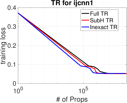
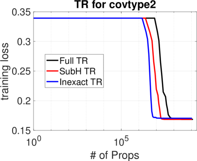
(a) Comparison between variants of TR algorithms

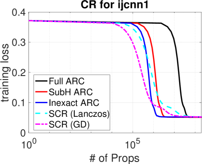
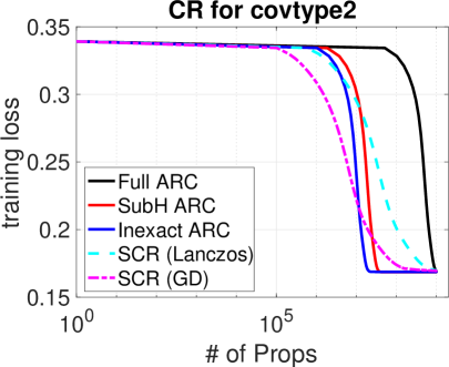
(b) Comparison between variants of CR algorithms

Figure 1: Performance of various methods on ijcnn1 and covertype for binary linear classification. The x-axis is drawn on the logarithmic scale.

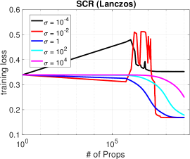
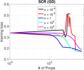
Figure 2: Robustness of Algorithm 2 and sensitivity of SCR w.r.t. the cubic regularization parameter on covertype dataset. For Algorithm 2, this parameter, initially set to $\sigma_{0}$, adaptively changes across iterations; while for SCR, it is kept fixed at a certain $\sigma$ for all iterations. (a) Robustness of Algorithm 2 to the choice of $\sigma_{0}$, where $\sigma_{0}$ varies over several orders of magnitude. (b)–(c) Sensitivity of SCR with two different sub-problem solvers (Lanczos and GD) and several choices of the fixed cubic regularization $\sigma$. For SCR (GD), the step size of GD for solving the sub-problem is hand-tuned to obtain the best performance (which can be extremely expensive).

The performance of the following methods are compared:

• Full TR/ARC: Standard TR and ARC algorithms with exact gradient and Hessian.

• SubH TR/ARC [50]: TR and ARC with exact gradient and sub-sampled Hessian.

• SCR (GD) [47]: CR with sub-sampled gradient and Hessian. The sub-problems are solved by gradient descent (GD) [7].

• SCR (Lanczos): CR which is similar to SCR (GD) [47] but the sub-problems are solved by generalized Lanczos method [8].

• Inexact TR/ARC (this work): TR and ARC with sub-sampled gradient and Hessian as described in Algorithms 1 and 2. The sub-problems of Algorithms 1 and 2 are solved, respectively, by CG-Steihaug [45], and by generalized Lanczos method [8].

Similar to [51], the performance of all the algorithms in our experiments is measured by tallying total number of propagations, i.e., number of oracle calls of function, gradient and Hessian-vector products. For all TR and ARC algorithms, we use the same setup in [51]. For all experiments, the gradient and Hessian sampling ratios are $10\%$ and $1\%$ of the entire dataset, respectively.

Computational Efficiency (Fig. 1):

First, we compare these Newton-type methods in terms of running time, as measured by the training loss versus total number of propagations; Fig. 1 depicts the results. For all variants of SCR, we hand-tuned the algorithm by performing an exhaustive grid-search over the involving hyper-parameters, and we show the best results. For all variants of TR and ARC, we choose the same initial parameters, i.e. trust region radius for TR and $\sigma_{0}$ for ARC.

We can observe that all methods achieve similar training errors, while Algorithms 1 and 2 do so with much fewer number of propagation calls, as compared with other members of their method class. For example, Inexact TR appears 3-5 times faster than SubH TR and 5-10 times faster than Full TR. Also, all variants of TR perform similarly, or better, than all variants of CR. This is an empirical evidence that the “optimal” worst-case analysis of CR, while theoretically interesting, might not translate to many practical applications of interest.

Robustness to Hyper-parameters (Fig. 2):

Next, we highlight the practical challenges arising with algorithms that heavily rely on the knowledge of hard-to-estimate parameters, and how this problem is solved by our methods since our algorithms are formulated so as not to need unknowable problem-related quantities. In particular, we aim here to demonstrate that an algorithm whose performance is greatly affected by different settings of parameters that cannot be easily estimated, lacks the versatility needed in many practical applications. To do so, we perform one such demonstration by focusing on sensitivity/robustness of Algorithm 2 and SCR [47] to the cubic regularization parameter $\sigma$.

Recall that a significant difference between Algorithm 2 and SCR is that, unlike the former, the latter requires many hyper-parameter tuning and knowledge of several quantities, e.g., regularization parameter $\sigma$ (which is kept fixed across iterations), Lipschitz constants of gradient and Hessian. The result is shown in Fig. 2. One can see that the performance of SCR is highly dependent the choice of its main hyper-parameter, i.e., $\sigma$. Indeed, if $\sigma$ is not chosen appropriately, SCR either converges very slowly or does not converge at all. To determine the appropriate value of $\sigma$ requires an expensive (in human time or CPU time) hyper-parameter search. This is in sharp contrast with Algorithm 2 which shows great robustness to the choice of $\sigma_{0}$ and works more-or-less “out of the box.”

5 Conclusions

In this paper, we considered inexact variants of trust region and adaptive cubic regularization in which, to increase efficiency, the gradient and Hessian, as well as the solution to the underlying sub-problems are all suitably approximated. Our algorithms, and their analysis, do not require knowledge of any unknowable parameter and hence, are easily implementable in practice. We showed that under mild conditions on all these approximation, to coverage to second-order criticality, the inexact variants achieve the same optimal iteration complexity as the exact counterparts. The advantages of our algorithms were also numerically demonstrated.

Acknowledgments.

MM gratefully acknowledges the support of DARPA, ONR, and the NSF. FR gratefully acknowledges the support of DARPA, the Australian Research Council through a Discovery Early Career Researcher Award (DE180100923) and the Australian Research Council Centre of Excellence for Mathematical and Statistical Frontiers (ACEMS).

Appendix A Proofs of the Main Theorems

Our proof techniques follow similar line of reasoning as in [34, 17, 8, 9, 50]. However, as alluded to in 1, the mild requirement on the gradient and Hessian approximations as in Condition 2 introduces many challenges. In the remainder of this section, we give the proof details of main results for Algorithms 1 and 2, respectively, in Section A.1 and LABEL:subsec:arc_opt1-A.2.

A.1 Proofs of TR results

The proof mainly follows [50, 17]. To bound the total iteration numbers, we need to show that the trust region radius never gets too small, i.e. $\Delta_{t}\geq\Delta_{lower}>0$ for all $t$; we do that in Lemma 12. For that we require some preliminary lemmas. Lemmas 7 and 8 gives the sufficient descent obtained with Cauchy and Eigen points. Lemma 9 shows the approximation error of $m_{t}(\mathbf{s}_{t})$ as predictor for $F(\mathbf{x}_{t}+\mathbf{s}_{t})-F(\mathbf{x}_{t})$. Using these lemmas, we then establish the upper bound on the total number of iterations, as in Lemma 13.

We now turn to more details. The following two lemmas could be found in [17], which establish 2.

Lemma 7 (Cauchy Points).

Suppose that $\mathbf{s}_{t}^{C}=\arg\min_{\|\alpha\mathbf{g}_{k}\|\leq\Delta_{t}}m_{t}(-\alpha\mathbf{g}_{t})$. Then we have

$$-m_{t}(\mathbf{s}_{t}^{C})\geq\frac{1}{2}\|\mathbf{g}_{t}\|\min\{\frac{\|\mathbf{g}_{t}\|}{1+\|\mathbf{H}_{t}\|},\Delta_{t}\}.$$ (14)

Lemma 8 (Eigen points).

When $\lambda_{\min}(\mathbf{H}_{t})$ is negative, suppose $\mathbf{u}_{t}$ satisfied

$$\langle\mathbf{g}_{t},\mathbf{u}_{t}\rangle\leq 0,~{}~{}~{}~{}and~{}~{}~{}~{}~{}\langle\mathbf{u}_{t},\mathbf{H}_{t}\mathbf{u}_{t}\rangle\leq-\nu|\lambda_{\min}(\mathbf{H}_{t})|\|\mathbf{u}_{t}\|^{2}.$$ (15)

Let $\mathbf{s}_{t}=\arg\min_{\|\mathbf{s}_{t}\|\leq\Delta_{t}}m_{t}(\alpha\mathbf{u}_{t})$, we have

$$-m_{t}(\mathbf{s}_{t})\geq\frac{\nu}{2}|\lambda_{\min}(\mathbf{H}_{t})|\|\mathbf{u}_{t}\|^{2}.$$ (16)

The above two lemmas show the descent that can be obtained by Cauchy and Eigen Points. The following lemma bounds the difference between the actual descent, i.e., $F(\mathbf{x}_{t}+\mathbf{s}_{t})-F(\mathbf{x}_{t})$, and the one predicted by $m(\mathbf{s}_{t})$.

Lemma 9.

Under Assumptions 1, we have

$$F(\mathbf{x}_{t}+\mathbf{s}_{t})-F(\mathbf{x}_{t})-m_{t}(\mathbf{x}_{t})\leq\langle\mathbf{s}_{t},\nabla F(\mathbf{x}_{t})-\mathbf{g}_{t}\rangle+\frac{1}{2}\delta_{H}\|\mathbf{s}_{t}\|^{2}+\frac{1}{2}L_{F}\|\mathbf{s}_{t}\|^{3}.$$ (17)

Proof.

Using taylor expansion of $F(\mathbf{x}_{t})$ at point $\mathbf{x}_{t}$,

$$F(\mathbf{x}_{t}+\mathbf{s}_{t})-F(\mathbf{x}_{t})-m_{t}(\mathbf{x}_{t}) =\langle\mathbf{s}_{t},\nabla F(\mathbf{x}_{t})-\mathbf{g}_{t})\rangle+\frac{1}{2}\langle\mathbf{s}_{t},(\nabla^{2}F(\mathbf{x}_{t}+\tau\mathbf{s}_{t})-\mathbf{H}_{t})\mathbf{s}_{t}\rangle$$

$$\leq\langle\mathbf{s}_{t},\nabla F(\mathbf{x}_{t})-\mathbf{g}_{t}\rangle+|\frac{1}{2}\langle\mathbf{s}_{t},(\mathbf{H}_{t}-\nabla^{2}\mathbf{F}(\mathbf{x}_{t}+\tau\mathbf{s}_{t}))\mathbf{s}_{t}\rangle|$$

$$\leq\langle\mathbf{s}_{t},\nabla F(\mathbf{x}_{t})-\mathbf{g}_{t}\rangle+|\frac{1}{2}\langle\mathbf{s}_{t},(\mathbf{H}_{t}-\nabla^{2}F(\mathbf{x}_{t}))\mathbf{s}_{t}\rangle|$$

$$~{}~{}~{}~{}~{}~{}~{}~{}~{}~{}~{}~{}~{}~{}~{}~{}~{}~{}~{}~{}~{}+|\frac{1}{2}\langle\mathbf{s}_{t},(\nabla^{2}F(\mathbf{x}_{t}+\tau\mathbf{s}_{t})-\nabla^{2}F(\mathbf{x}_{t}))\mathbf{s}_{t}\rangle|$$

$$\leq\langle\mathbf{s}_{t},\nabla F(\mathbf{x}_{t})-\mathbf{g}_{t}\rangle+\frac{1}{2}\delta_{H}\|\mathbf{s}_{t}\|^{2}+\frac{1}{2}L_{F}\|\mathbf{s}_{t}\|^{3},$$

where $\tau\in[0,1]$. When $\|\mathbf{g}_{t}\|>\epsilon_{g}$, we can get a loose bound for (17)

$$|F(\mathbf{x}_{t}+\mathbf{s}_{t})-F(\mathbf{x}_{t})-m_{t}(\mathbf{x}_{t})|\leq\delta_{g}\Delta_{t}+\frac{1}{2}\delta_{H}\Delta_{t}^{2}+\frac{1}{2}L_{F}\Delta_{t}^{3}.$$ (18)

∎

By combining Lemmas 9 and 18, Lemma 10 guarantees that, in case $\|\mathbf{g}_{t}\|\geq\epsilon_{g}$, the iteration is successful and the update is accepted.

Lemma 10.

Given Assumption 1 and 2, and Condition 1 and 2, suppose at iteration $t$, $\|\mathbf{g}_{t}\|\geq\epsilon_{g}$ and δ_g ¡ 1-η4ϵ_g,  Δ_t≤min{ϵg1 + KH, (1-η)ϵg12LH, (1-η)ϵg3}, then the iteration t is successful, i.e. $\Delta_{t+1}=\gamma\Delta_{t}$.

Proof.

First, by Condition 2, Lemma 7 and $\|\mathbf{g}_{t}\|\geq\epsilon_{g}$, we have,

$$-m_{t}(\mathbf{s}_{t}) \geq\frac{1}{2}\|\mathbf{g}_{t}\|\min\{\frac{\|\mathbf{g}_{t}\|}{1+\|\mathbf{H}_{t}\|},\Delta_{t}\}$$

$$\geq\frac{1}{2}\|\mathbf{g}_{t}\|\min\{\frac{\epsilon_{g}}{1+\|\mathbf{H}_{t}\|},\Delta_{t}\}$$

$$=\frac{1}{2}\epsilon_{g}\Delta_{t}.$$

Now according to Lemma 9, we have

$$1-\rho_{t} =\frac{F(\mathbf{x}_{t}+\mathbf{s}_{t})-F(\mathbf{x}_{t})-m_{t}(\mathbf{s}_{t})}{-m_{t}(\mathbf{s}_{t})}$$

$$\leq\frac{\delta_{g}\Delta_{t}+\frac{1}{2}\delta_{H}\Delta_{t}^{2}+\frac{1}{2}L_{F}\Delta_{t}^{3}}{\frac{1}{2}\epsilon_{g}\Delta_{t}}$$

$$=2\frac{\delta_{g}}{\epsilon_{g}}+\frac{\delta_{h}}{\epsilon_{g}}\Delta_{t}+\frac{L_{F}}{\epsilon_{g}}\Delta_{t}^{2}$$

$$\leq\frac{1-\eta}{2}+\frac{\delta_{H}}{\epsilon_{g}}\Delta_{t}+\frac{L_{F}}{\epsilon_{g}}\Delta_{t}^{2}.$$

Since $\delta_{H}<1$, it follows -δH+δH2+2LH(1-η)ϵg2LH ≥-1+1+2LH(1-η)ϵg2LH. Now, we consider two cases. If $2L_{H}(1-\eta)\epsilon_{g}\leq 1$, it is not hard to show that -1+1+2L_H(1-η)ϵ_g ≥2LH(1-η)ϵg3. Otherwise, if $2L_{H}(1-\eta)\epsilon_{g}>1$, then it can be shown that -1+1+2L_H(1-η)ϵ_g ≥LH(1-η)ϵg3. By assumption $\Delta_{t}\leq\min\{\sqrt{\frac{(1-\eta)\epsilon_{g}}{12L_{H}}},\frac{(1-\eta)\epsilon_{g}}{3}\}$, it follows, 1 - ρ_t ≤1-η2 + δHϵg Δ_t+ LFϵg Δ_t^2 ≤1 - η, which implies that the iteration $t$ is successful. ∎

Dealing with the first order term in Eq. 17 is particularly challenging when $\|\mathbf{g}_{t}\|<\epsilon_{g}$. If we simply substitute the result of Lemma 11, i.e. $-m_{t}(\mathbf{s}_{t}^{E})=\operatorname{\mathcal{O}}(\lambda_{\min}(\mathbf{H}_{t}))$ in $1-\rho_{t}$, it is not hard to see we need to bound a term as $c{\epsilon_{g}}/{\epsilon_{H}}$, which indicates $\epsilon_{H}\gg\epsilon_{g}$. That is unacceptable. Therefore, after getting Eigen Points $\mathbf{s}_{t}^{E}$, we can use either of $\mathbf{s}_{t}=\mathbf{s}_{t}^{E}$ or $\mathbf{s}_{t}=-\mathbf{s}_{t}^{E}$, which gives larger descent. By this simple trick, we could drop $\langle\mathbf{s}_{t},\nabla F(\mathbf{x}_{t})\rangle$ in our proof; see following lemma for more details.

Lemma 11.

Given Assumption 1 and 2, and Condition 1 and 2, suppose at iteration $t$, $\|\mathbf{g}_{t}\|<\epsilon_{g}$ and $\lambda_{\min}(H_{t})<-\epsilon_{H}$. Then according to (5) m_t(s) = 12 ⟨s,H_ts⟩, and according to (16), $\mathbf{s}_{t}$ satisfies, -m_t(s_t) ≥-m_t(s_t^E) ≥ν2—λ_min(H_t)—Δ_t^2. If $\delta_{H}<\dfrac{1-\eta}{2}\nu\epsilon_{H},\Delta_{t}\leq(1-\eta)\dfrac{\nu\epsilon_{H}}{L_{F}}$, then the iteration $t$ is successful, i.e. $\Delta_{t+1}=\gamma\Delta_{t}$.

Proof.

First, review (17),

$$F(\mathbf{x}_{t}+\mathbf{s}_{t})-F(\mathbf{x}_{t})-m_{t}(\mathbf{x}_{t}) \leq\langle\mathbf{s}_{t},\nabla F(\mathbf{x}_{t})\rangle+\frac{1}{2}\delta_{H}\|\mathbf{s}_{t}\|^{2}+\frac{1}{2}L_{F}\|\mathbf{s}_{t}\|^{3}.$$

Since either $\mathbf{s}_{t}$ or $-\mathbf{s}_{t}$ could be a searching direction, at least one of ⟨s_t, ∇F(x_t)⟩ ≤0      or      ⟨-s_t, ∇F(x_t)⟩ ≤0 is true. W.l.o.g, assume $\langle\mathbf{s}_{t},\nabla F(\mathbf{x}_{t})\rangle\leq 0$. Then

$$F(\mathbf{x}_{t}+\mathbf{s}_{t})-F(\mathbf{x}_{t})-m_{t}(\mathbf{x}_{t}) \leq\frac{1}{2}\delta_{H}\|\mathbf{s}_{t}\|^{2}+\frac{1}{2}L_{F}\|\mathbf{s}_{t}\|^{3}$$

Therefore,

$$1-\rho_{t} =\frac{F(\mathbf{x}_{t}+\mathbf{s}_{t})-F(\mathbf{x}_{t})-m_{t}(\mathbf{s}_{t})}{-m_{t}(\mathbf{s}_{t})}$$

$$\leq\frac{\frac{1}{2}\delta_{H}\|\mathbf{s}_{t}\|^{2}+\frac{1}{2}L_{F}\|\mathbf{s}_{t}\|^{3}}{\frac{\nu}{2}|\lambda_{\min}(\mathbf{H}_{t})|\Delta_{t}^{2}}$$

$$\leq\frac{\frac{1}{2}\delta_{H}\|\mathbf{s}_{t}\|^{2}+\frac{1}{2}L_{F}\|\mathbf{s}_{t}\|^{3}}{\frac{\nu}{2}\epsilon_{H}\Delta_{t}^{2}}$$

$$\leq\frac{\frac{1}{2}\delta_{H}\Delta_{t}^{2}+\frac{1}{2}L_{F}\Delta_{t}^{3}}{\frac{\nu}{2}\epsilon_{H}\Delta_{t}^{2}}$$

$$=\frac{\delta_{H}}{\nu\epsilon_{H}}+\frac{L_{F}\Delta_{t}}{\nu\epsilon_{H}}$$

$$<(1-\eta)/2+(1-\eta)/2$$

$$<1-\eta,$$

where the last second inequality uses the condition of $\delta_{H}$ and $\Delta_{t}$. Therefore, $\rho_{t}\geq\eta$ and the iteration is successful. ∎

Based on Lemmas 11 and 10, the following lemma helps to get the lower bound of $\Delta_{t}$, whose proof could be found in [50].

Lemma 12.

Under Assumption 1 and A.2, Condition C.1, and δ_g ¡ 1-η4ϵ_g,     δ_H ¡min{ 1-η2νϵ_H,1}. for Algorithm we have for all t, Δ_t≥1γ min{ϵg1 + KH, (1-η)ϵg12LH, (1-η)ϵg3, νϵHLF}

As a consequence, we now can give the upper bound of successful iterations.

Lemma 13 (Successful iterations).

Given Assumption 1 and 2, and Condition 1 and 2, let $\mathscr{T}_{\text{succ}}$ denote the set of all the successful iterations before Algorithm stops. The the number of successful iterations is upper bounded by —T_succ— ≤F(x0) - F(x*)CϵHmin{ϵg2, ϵH2}, where $C$ is a constant depending on $L_{F},K_{H},\delta_{g},\delta_{H},\eta,\nu$.

Proof.

Suppose Algorithm 1 doesn’t terminate at iteration $t$. Then either $\|\mathbf{g}_{t}\|\geq\epsilon_{g}$ or $\lambda_{\min}(\mathbf{H}_{t})\leq-\epsilon_{H}$. If $\|\mathbf{g}_{t}\|\geq\epsilon_{g}$, according to (14), we have

$$-m_{t}(\mathbf{s}_{t}) \geq\frac{1}{2}\|\mathbf{g}_{t}\|\min\{\frac{\|\mathbf{g}_{t}\|}{1+\|\mathbf{H}_{t}\|},\Delta_{t}\}$$

$$\geq\frac{1}{2}\epsilon_{g}\min\{\frac{\epsilon_{g}}{1+K_{H}},C_{0}\epsilon_{g},C_{1}\epsilon_{H}\}$$

$$\geq C_{2}\epsilon_{g}\min\{\epsilon_{g},\epsilon_{H}\}$$

Similialy, in the second case $\lambda_{\min}(\mathbf{H}_{t})\leq-\epsilon_{H}$, from (16), -m_t(s_t) ≥12ν∥λ_min(H_t)∥Δ_t^2≥C_3ϵ_Hmin{ϵ_g^2, ϵ_H^2}. Since $F(\mathbf{x})$ is monotonically decreasing, we have

$$F(\mathbf{x}_{0})-F(\mathbf{x}^{*}) \geq\sum_{t=0}^{\infty}F(\mathbf{x}_{t})-F(\mathbf{x}_{t+1})$$

$$\geq\sum_{t\in\mathscr{T}_{\text{succ}}}F(\mathbf{x}_{t})-F(\mathbf{x}_{t+1})$$

$$\geq\eta\sum_{t\in\mathscr{T}_{\text{succ}}}C_{3}\epsilon_{H}\min\{\epsilon_{g}^{2},\epsilon_{H}^{2}\}$$

$$\geq\left|\mathscr{T}_{\text{succ}}\right|C_{3}\epsilon_{H}\min\{\epsilon_{g}^{2},\epsilon_{H}^{2}\}.$$

Since one of the aboves cases must happen for a successful iteration, it follows, —T_succ— ≤F(x0) - F(x*)C3ϵHmin{ϵg2, ϵH2}. ∎

Using the above lemma, the proof of following theorem could be found in [50]. See 2

A.2 Proof for Inexact ARC

In this section, we will prove Theorem 3. The goal is to bound the total number of iterations of Algorithm 2 before it terminates. First let’s denote $\mathscr{T}_{\text{succ}}$ as the set of all the successful iteration and $\mathscr{T}_{\text{fail}}$ as the set of all the failure iterations. Now we will upper bound the iteration complexity $T:=\left|\mathscr{T}_{\text{succ}}\right|+\left|\mathscr{T}_{\text{fail}}\right|$.

First we present the following lemma that gives an upper bound of $\left|\mathscr{T}_{\text{fail}}\right|$.

Lemma 14.

In Algorithm 2, suppose we have $\sigma_{t}\leq C$, where $C$ is some constant, for all the iteration $t$ before it stops. Then we have $\left|\mathscr{T}_{\text{fail}}\right|\leq\left|\mathscr{T}_{\text{succ}}\right|+\operatorname{\mathcal{O}}(1)$.

Proof.

Since $\sigma_{t}\leq C$, then $\sigma_{T}=\sigma_{0}\gamma^{\left|\mathscr{T}_{\text{succ}}\right|-\left|\mathscr{T}_{\text{fail}}\right|}\leq C$. Then immediately we obtain —T_fail— ≤log(C/σ_0)/logγ+ —T_fail— = —T_fail— + O(1). ∎

Now the remaining analysis is first to show indeed there is a uniform upper bound for all $\sigma_{t}$ and second to bound number of all the successful iterations.

Following [50], we have a similar Lemma  15 as [50, Lemma 15 ].

Lemma 15 (Cauchy Point).

When $\|\mathbf{g}_{t}\|\geq\epsilon_{g}$, let s_t^C = argmin_α≥0 m_t(-αg_t). Then we have

$$\|\mathbf{s}_{t}^{C}\| =\frac{1}{2\sigma_{t}}(\sqrt{K_{t}^{2}+4\sigma_{t}\|\mathbf{g}_{t}\|}-K_{t}).$$ (19a)

$$-m_{t}(\mathbf{s}_{t}^{C}) \geq\max\left\{\frac{1}{12}\|\mathbf{s}_{t}^{C}\|^{2}(\sqrt{K_{t}^{2}+4\sigma_{t}\|\mathbf{g}_{t}\|}-K_{t}),\frac{\|\mathbf{g}_{t}\|}{2\sqrt{3}}\min\{\frac{\|\mathbf{g}_{t}\|}{|K_{t}|},\frac{\|\mathbf{g}_{t}\|}{\sqrt{\sigma_{t}\|\mathbf{g}_{t}\|}}\}\right\},$$ (19b)

where $K_{t}=\frac{\langle\mathbf{H}_{t}\mathbf{g}_{t},\mathbf{g}_{t}\rangle}{\|\mathbf{g}_{t}\|^{2}}$.

Proof.

First, we have ⟨g_t,s_t^C⟩ + ⟨s_t^C, H_ts_t^C⟩ + σ_t∥s_t^C∥^3=0. Since $\mathbf{s}_{t}^{C}=-\alpha\mathbf{g}_{t}$ for some $\alpha>0$, -α∥g_t∥^2 + α^2 ⟨g_t, H_tg_t⟩ + σ_tα^3∥g_t∥^3=0. We can find explicit formula for such $\alpha$ by finding the roots of the quadratic function r(α) = -∥g_t∥^2 + α⟨g_t, H_tg_t⟩ + σ_tα^2∥g_t∥^3. We have α= ⟨gt, Htgt⟩ + ⟨gt, Htgt⟩2+ 4σt∥gt∥52σt∥gt∥3, and 2ασ_t∥g_t∥ = (K_t^2 + 4σ_t∥g_t∥ - K_t. Hence, it follows that

$$\|\mathbf{s}_{t}^{C}\|=\alpha\|\mathbf{g}_{t}\|=\frac{1}{2\sigma_{t}}(\sqrt{K_{t}^{2}+4\sigma_{t}\|\mathbf{g}_{t}\|}-K_{t}).$$

Now, from [10, Lemma 2.1 ], we get -m

References

• [1] Afonso S Bandeira, Katya Scheinberg and Luís N Vicente “Convergence of trust-region methods based on probabilistic models” In SIAM Journal on Optimization 24.3 SIAM, 2014, pp. 1238–1264
• [2] Albert S Berahas, Raghu Bollapragada and Jorge Nocedal “An Investigation of Newton-Sketch and Subsampled Newton Methods” In arXiv preprint arXiv:1705.06211, 2017
• [3] Dimitri P. Bertsekas “Nonlinear programming” Athena scientific, 1999
• [4] Jose Blanchet, Coralia Cartis, Matt Menickelly and Katya Scheinberg “Convergence rate analysis of a stochastic trust region method for nonconvex optimization” In arXiv preprint arXiv:1609.07428, 2016
• [5] Raghu Bollapragada, Richard Byrd and Jorge Nocedal “Exact and Inexact Subsampled Newton Methods for Optimization” In arXiv preprint arXiv:1609.08502, 2016
• [6] Stephen Boyd and Lieven Vandenberghe “Convex optimization” Cambridge university press, 2004
• [7] Yair Carmon and John C Duchi “Gradient Descent Efficiently Finds the Cubic-Regularized Non-Convex Newton Step” In arXiv preprint arXiv:1612.00547, 2016
• [8] Coralia Cartis, Nicholas IM Gould and Philippe L Toint “Adaptive cubic regularisation methods for unconstrained optimization. Part I: motivation, convergence and numerical results” In Mathematical Programming 127.2 Springer, 2011, pp. 245–295
• [9] Coralia Cartis, Nicholas IM Gould and Philippe L Toint “Adaptive cubic regularisation methods for unconstrained optimization. Part II: worst-case function-and derivative-evaluation complexity” In Mathematical programming 130.2 Springer, 2011, pp. 295–319
• [10] Coralia Cartis, Nicholas IM Gould and Philippe L Toint “Complexity bounds for second-order optimality in unconstrained optimization” In Journal of Complexity 28.1 Elsevier, 2012, pp. 93–108
• [11] Coralia Cartis, Nicholas IM Gould and Philippe L Toint “On the complexity of steepest descent, Newton’s and regularized Newton’s methods for nonconvex unconstrained optimization problems” In Siam journal on optimization 20.6 SIAM, 2010, pp. 2833–2852
• [12] Coralia Cartis, Nicholas IM Gould and Philippe L Toint “Optimal Newton-type methods for nonconvex smooth optimization problems”, 2011
• [13] Chih-Chung Chang and Chih-Jen Lin “LIBSVM: A library for support vector machines” Software available at http://www.csie.ntu.edu.tw/~cjlin/libsvm In ACM Transactions on Intelligent Systems and Technology 2, 2011, pp. 27:1–27:27
• [14] Ruobing Chen, Matt Menickelly and Katya Scheinberg “Stochastic optimization using a trust-region method and random models” In arXiv preprint arXiv:1504.04231, 2015
• [15] Anna Choromanska, Mikael Henaff, Michael Mathieu, Gérard Ben Arous and Yann LeCun “The loss surfaces of multilayer networks” In Artificial Intelligence and Statistics, 2015, pp. 192–204
• [16] Andrew R Conn, Katya Scheinberg and Luís N Vicente “Global convergence of general derivative-free trust-region algorithms to first-and second-order critical points” In SIAM Journal on Optimization 20.1 SIAM, 2009, pp. 387–415
• [17] Andrew R Conn, Nicholas IM Gould and Philippe L Toint “Trust region methods” SIAM, 2000
• [18] Yann N Dauphin, Razvan Pascanu, Caglar Gulcehre, Kyunghyun Cho, Surya Ganguli and Yoshua Bengio “Identifying and attacking the saddle point problem in high-dimensional non-convex optimization” In Advances in neural information processing systems, 2014, pp. 2933–2941
• [19] Kenji Fukumizu and Shun-ichi Amari “Local minima and plateaus in hierarchical structures of multilayer perceptrons” In Neural Networks 13.3 Elsevier, 2000, pp. 317–327
• [20] Rong Ge, Furong Huang, Chi Jin and Yang Yuan “Escaping From Saddle Points-Online Stochastic Gradient for Tensor Decomposition.” In COLT, 2015, pp. 797–842
• [21] S Gratton, CW Royer, LN Vicente and Z Zhang “Complexity and global rates of trust-region methods based on probabilistic models”, 2017
• [22] Andreas Griewank “Some bounds on the complexity of gradients, Jacobians, and Hessians” In Complexity in numerical optimization World Scientific, 1993, pp. 128–162
• [23] Kaiming He, Xiangyu Zhang, Shaoqing Ren and Jian Sun “Deep residual learning for image recognition” In Proceedings of the IEEE Conference on Computer Vision and Pattern Recognition, 2016, pp. 770–778
• [24] Xi He, Dheevatsa Mudigere, Mikhail Smelyanskiy and Martin Takác “Large scale distributed hessian-free optimization for deep neural network” In arXiv preprint arXiv:1606.00511, 2016
• [25] Christopher J Hillar and Lek-Heng Lim “Most tensor problems are NP-hard” In Journal of the ACM (JACM) 60.6 ACM, 2013, pp. 45
• [26] Chi Jin, Rong Ge, Praneeth Netrapalli, Sham M Kakade and Michael I Jordan “How to Escape Saddle Points Efficiently” In arXiv preprint arXiv:1703.00887, 2017
• [27] Ryan Kiros “Training neural networks with stochastic Hessian-free optimization” In arXiv preprint arXiv:1301.3641, 2013
• [28] Jonas Moritz Kohler and Aurelien Lucchi “Sub-sampled Cubic Regularization for Non-convex Optimization” In arXiv preprint arXiv:1705.05933, 2017
• [29] Jeffrey Larson and Stephen C Billups “Stochastic derivative-free optimization using a trust region framework” In Computational Optimization and Applications 64.3 Springer, 2016, pp. 619–645
• [30] Yann A LeCun, Léon Bottou, Genevieve B Orr and Klaus-Robert Müller “Efficient backprop” In Neural networks: Tricks of the trade Springer, 2012, pp. 9–48
• [31] Kfir Y Levy “The Power of Normalization: Faster Evasion of Saddle Points” In arXiv preprint arXiv:1611.04831, 2016
• [32] James Martens “Deep learning via Hessian-free optimization” In International Conference on Machine Learning (ICML), 2010
• [33] Katta G Murty and Santosh N Kabadi “Some NP-complete problems in quadratic and nonlinear programming” In Mathematical programming 39.2 Springer, 1987, pp. 117–129
• [34] Yurii Nesterov “Cubic regularization of Newton’s method for convex problems with constraints”, 2006
• [35] Yurii Nesterov “Introductory lectures on convex optimization” Springer Science & Business Media, 2004
• [36] Yurii Nesterov and Boris T Polyak “Cubic regularization of Newton method and its global performance” In Mathematical Programming 108.1 Springer, 2006, pp. 177–205
• [37] Jorge Nocedal and Stephen Wright “Numerical optimization” Springer Science & Business Media, 2006
• [38] Barak A Pearlmutter “Fast exact multiplication by the Hessian” In Neural computation 6.1 MIT Press, 1994, pp. 147–160
• [39] Mert Pilanci and Martin J. Wainwright “Newton Sketch: a linear-time optimization algorithm with linear-quadratic convergence” In arXiv preprint arXiv:1505.02250, 2015
• [40] Jeffrey Regier, Michael I Jordan and Jon McAuliffe “Fast Black-box Variational Inference through Stochastic Trust-Region Optimization” In arXiv preprint arXiv:1706.02375, 2017
• [41] Farbod Roosta-Khorasani and Michael W. Mahoney “Sub-sampled Newton methods I: globally convergent algorithms” In arXiv preprint arXiv:1601.04737, 2016
• [42] Farbod Roosta-Khorasani and Michael W Mahoney “Sub-sampled Newton methods II: local convergence rates” In arXiv preprint arXiv:1601.04738, 2016
• [43] Andrew M Saxe, James L McClelland and Surya Ganguli “Exact solutions to the nonlinear dynamics of learning in deep linear neural networks” In arXiv preprint arXiv:1312.6120, 2013
• [44] Sara Shashaani, Fatemeh Hashemi and Raghu Pasupathy “ASTRO-DF: A Class of Adaptive Sampling Trust-Region Algorithms for Derivative-Free Stochastic Optimization” In arXiv preprint arXiv:1610.06506, 2016
• [45] Trond Steihaug “The conjugate gradient method and trust regions in large scale optimization” In SIAM Journal on Numerical Analysis 20.3 SIAM, 1983, pp. 626–637
• [46] Grzegorz Swirszcz, Wojciech Marian Czarnecki and Razvan Pascanu “Local minima in training of deep networks” In arXiv preprint arXiv:1611.06310, 2016
• [47] Nilesh Tripuraneni, Mitchell Stern, Chi Jin, Jeffrey Regier and Michael I Jordan “Stochastic Cubic Regularization for Fast Nonconvex Optimization” In arXiv preprint arXiv:1711.02838, 2017
• [48] Oriol Vinyals and Daniel Povey “Krylov Subspace Descent for Deep Learning” In AISTATS, 2012, pp. 1261–1268
• [49] Simon Wiesler, Jinyu Li and Jian Xue “Investigations on Hessian-free optimization for cross-entropy training of deep neural networks” In INTERSPEECH, 2013, pp. 3317–3321
• [50] Peng Xu, Farbod Roosta-Khorasani and Michael W. Mahoney “Newton-Type Methods for Non-Convex Optimization Under Inexact Hessian Information” In arXiv preprint arXiv:1708.07164, 2017
• [51] Peng Xu, Farbod Roosta-Khorasani and Michael W. Mahoney “Second-Order Optimization for Non-Convex Machine Learning: An Empirical Study” In arXiv preprint arXiv:1708.07827, 2017
• [52] Peng Xu, Jiyan Yang, Farbod Roosta-Khorasani, Christopher Ré and Michael W Mahoney “Sub-sampled newton methods with non-uniform sampling” In Advances in Neural Information Processing Systems, 2016, pp. 3000–3008