Perturbative unitarity and higher-order Lorentz symmetry breaking

Abstract

We study perturbative unitarity in the scalar sector of the Myers-Pospelov model. The model introduces a preferred four-vector $n$ which breaks Lorentz symmetry and couples to a five-dimension operator. When the preferred four-vector is chosen in the pure timelike or lightlike direction, the model becomes a higher time derivative theory, leading to a cubic dispersion relation. Two of the poles are shown to be perturbatively connected to the standard ones, while a third pole, which we call the Lee-Wick-like pole, is associated to a negative metric, in Hilbert space, threatening the preservation of unitarity. The pure spacelike case is a normal theory in the sense that it has only two solutions both being small perturbations over the standard ones. We analyze perturbative unitarity for purely spacelike and timelike cases using the optical theorem and considering a quartic self-interaction term. By computing discontinuities in the loop diagram, we arrive at a pinching condition which determines the propagation of particles and Lee-Wick-like particles through the cut. We find that the contribution for Lee-Wick-like particles vanishes for any external momenta, leaving only the contribution of particles, thus preserving one-loop unitarity in both cases.

I Introduction

The breakdown of Lorentz symmetry at the Planck mass scale $m_{P}=10^{19}$ GeV has been intensively studied in the last two decades. Many efforts have been put forward in order to provide experimental input for these quantum gravity effects. The detection of such possible new physics, however, has been very challenging principally because the high scale imposes a strong suppression. In particular, at present-time colliders with attainable energies of $m\sim 13$ TeV, these effects may be suppressed by some power of $m/m_{P}\sim 10^{-15}$, which is very small. Moreover, for experiments using the highest-energy cosmic rays observed, they are about eight orders of magnitude below the Planck mass. $CPT$ and Lorentz symmetry departures have received motivation from various sources, specially from attempts to construct a quantum gravity theory QGV .

The effective approach, encoding the high scale $\Lambda$, has shown to be a powerful method to explore such departures. One advantage is that it allows us to include the most general form of Lorentz invariance violation, without resorting to a particular theory or method of calculation to get down to a low-energy model. Many of these studies have been given within the effective framework of the standard model extension (SME) SME . The SME encompasses all the possible effective terms describing Lorentz symmetry violation in matter and gravity sectors. It is implemented through constant coefficients which couple to operators of renormalizable mass dimension in the minimal sector and to higher-order mass dimension operators in the nonminimal sector SME-nonminimal . The coefficients are believed to arise as expectation values of tensor fields possibly from spontaneous Lorentz violation in a more fundamental theory. The strong bounds on these parameters in the minimal sector has prompted the exploration at higher energies using higher-order operators MP . Limits on the Lorentz violating coefficients of nonrenormalizable operators have been obtained from astrophysical observations MP_Limits and synchrotron radiation syn ; see also comp . Recently, extensions with higher-order couplings have also been proposed H-O-C .

One theoretical advantage of introducing higher-order operators is that ultraviolet divergencies of conventional quantum field theories can be softened Rad-Corr ; dim5 . However, as is well known, in many cases this comes with the appearance of an indefinite-metric Hilbert space, leading to a possible loss of conservation of probability or nonunitarity of the $S$ matrix PU . Many of the problems have been analyzed and resolved in the framework developed by Lee and Wick Lee-Wick , in which the asymptotic space is restricted to contain only stable particles with positive metric. Further studies to deal with amplitudes in a covariant fashion and their nonanalytic pinching within an ad hoc prescription, were developed in Cut . The indefinite metric approach has also been used to improve the hierarchy problem in the scalar sector of the standard model G . Recently, it has been shown that Lee-Wick theories can be interpreted as nonanalytic Wick rotated Euclidean theories Ans-Piva . Here, we study unitarity in a Lorentz violating model with higher-order operators in light of the Lee-Wick studies unit-LW . The class of higher time derivative field theories that we consider extends the notion of Lee-Wick theory due to the explicit noncovariance, which may be reflected by the absence of complex conjugate ghost poles. Previous studies for tree level unitarity have been given in unit .

Another focus, recently discussed in Ext-leg ; dens , concerns the effect of Lorentz violating radiative corrections in tree level physics. It has been shown that external leg physics gets modified due to the appearance of observer Lorentz scalars in the spectral density function dens . A particular model of the SME has been analyzed and the corresponding modification for asymptotic fields has been found Ext-leg . Extensions to include higher-order Lorentz violation have been given in ren .

The organization of this paper is as follows. In Sec. II, we introduce the scalar Myers-Pospelov model with dimension-five operators. We found the dispersion relations for the purely spacelike, purely timelike, and lightlike cases. We analyze the solutions in the three cases and found that for certain values of space momenta, some solutions become complex, making the poles of the propagators move to the complex energy plane. In all of the cases, we identify perturbative solutions and those belonging to the Lee-Wick-like class with an associated negative metric. In Sec. III, we prove the conservation of unitarity for the purely spacelike and timelike cases at one-loop order using the optical theorem and focusing on a quartic interaction term. Finally, in Sec. IV, we give our final remarks and conclusions.

II Effective model

Our model is based on the Lorentz violating extension Myers-Pospelov Lagrangian density in the scalar sector MP :

$$\mathcal{L} = \partial_{\mu}\Phi^{*}\partial^{\mu}\Phi-m^{2}\Phi^{*}\Phi+ig\Phi^{*}(n\cdot\partial)^{3}\Phi+\mathcal{L}_{\text{int}}\,,$$ (1)

where

$$\mathcal{L}_{\text{int}} = \frac{\lambda}{4!}(\Phi^{*}\Phi)^{2}\,.$$ (2)

Here $g$ is a Planck mass suppressed constant and $n$ a preferred four-vector which characterizes the type of Lorentz violation. When $n$ has a temporal component, the theory belongs to a class of theory better known as higher time derivative theory. As we will show further in this case the theory displays an additional degree of freedom.

To begin with, let us consider a general preferred four-vector $n$ with a free equation of motion ($\lambda=0$):

$$\left(\Box+m^{2}-ig\left(n\cdot\partial\right)^{3}\right)\Phi=0\,.$$ (3)

Using the plane wave ansatz $\Phi(x)\sim\int dp\,\Phi(p)e^{-ipx}$ yields the dispersion relation

$$p^{2}-m^{2}-g(n\cdot p)^{3}=0\,.$$ (4)

Now we can specialize to the different cases. Let us begin with a pure spacelike four-vector $n=(0,\vec{n})$, where the dispersion relation takes the form

$$p_{0}^{2}-E_{p}^{2}+g(\vec{n}\cdot\vec{p})^{3}=0\,,$$ (5)

where $E_{p}=\sqrt{\vec{p}^{2}+m^{2}}$. The solutions are $p_{0}=\pm\omega_{s}$ with

$$\omega_{s}=\sqrt{E_{p}^{2}-g(\vec{n}\cdot\vec{p})^{3}}\,.$$ (6)

Without loss of generality we take $g>0$ and define the function

$$f(|\vec{p}|) = |\vec{p}|^{2}+m^{2}-a|\vec{p}|^{3}\,,$$ (7)

with

$$a(\theta)=g|\vec{n}|^{3}\cos^{3}\theta$$ (8)

where $\theta$ is the angle between $\vec{n}$ and $\vec{p}$.

When $0\leq\theta<\pi/2$, and so $a>0$, some solutions become complex at higher momenta than $|\vec{p}|>\mathcal{P}$, where we define

$$\mathcal{P} = \frac{1}{3a}\left(1+\left(\frac{1+i\sqrt{3}}{2}\right)Q^{-1/3}+\left(\frac{1-i\sqrt{3}}{2}\right)Q^{1/3}\right)\,,$$ (9)

with

$$Q = \frac{1}{2}\left(b+\sqrt{b^{2}-4}\right)\,,$$

$$b = -2-27a^{2}m^{2}\,.$$ (10)

One can show that for $gm\ll|\vec{n}|^{-3}\cos^{-3}\theta$, the approximation gives

$$\mathcal{P}\approx\frac{1}{g|\vec{n}|^{3}\cos^{3}\theta}+gm^{2}|\vec{n}|^{3}\cos^{3}\theta\,,$$ (11)

which indeed is very high for any angle $\theta$ in the interval. In contrast, at directions $\pi/2<\theta\leq\pi$, the solutions $\omega_{s}$ are always real. For the particular value at $\theta=\pi/2$, we have a blind direction at which we recover the usual dispersion relation.

In our concordant frame which follows from the condition imposed on $g$, there may be instabilities due to complex solutions that arise for higher values than $\mathcal{P}$, but also instabilities related to spacelike states K-R . This is true even imposing the cutoff $\mathcal{P}$, since then highly boosted frames with real momenta can produce negative energies. As an example, consider $n=(n_{0},0,0,n_{3})$ and the corresponding spacelike state $p=(0,0,0,p_{3}^{\pm})$,

$$p_{3}^{\pm}=\frac{gn_{3}}{2}\pm\sqrt{\left(\frac{gn_{3}}{2}\right)^{2}-m^{2}}\,,$$ (12)

which is a solution of the dispersion relation (5).

A more general analysis follows by considering the velocity group $v_{g}$,

$$v_{g}=\frac{2|\vec{p}|+3a|\vec{p}|^{2}}{2\sqrt{|\vec{p}|^{2}+m^{2}+a|\vec{p}|^{3}}}\,,$$ (13)

where we expect instabilities (provided interactions are turned on) and small deviations from microcausality as seen in the limit $v_{g}\to\infty$ for $|\vec{p}|\to\infty$, see  K-R . Recently, it has been shown that an extended Hamiltonian formalism allows us to implement a consistent canonical quantization for Lorentz violating theories containing spacelike states Neg-En .

It is not difficult to find the propagator

$$i\Delta(p_{0},\vec{p},\epsilon) = \frac{i}{(p_{0}-\omega+i\epsilon)(p_{0}+\omega-i\epsilon)}\,,$$ (14)

where the location of poles is the standard one.

Now we continue with a purely timelike four-vector $n=(1,0,0,0)$. It yields the dispersion relations

$$p_{0}^{2}-E_{p}^{2}-gp_{0}^{3}=0\,.$$ (15)

Solving (15) we find the exact three solutions

$$\omega_{1} = \frac{1}{3g}\left(1+\xi^{-1/3}z_{0}+\xi^{1/3}z_{0}^{*}\right)\,,$$

$$\omega_{2} = \frac{1}{3g}\left(1-\xi^{-1/3}-\xi^{1/3}\right)\,,$$ (16)

$$W = \frac{1}{3g}\left(1+\xi^{-1/3}z_{0}^{*}+\xi^{1/3}z_{0}\right)\,,$$

where we have introduced $z_{0}=e^{-\frac{i\pi}{3}}$ and defined the expressions

$$\xi = \frac{1}{2}(\beta+\sqrt{\beta^{2}-4})\,,$$

$$\beta = -2+27g^{2}E_{p}^{2}\,.$$ (17)

In complex energy-plane in terms of momenta $|\vec{p}|$, the solutions move according to Fig.1. In an analogous way, the solutions for the field $\Phi^{*}$ are obtained by the replacement $g\to-g$.

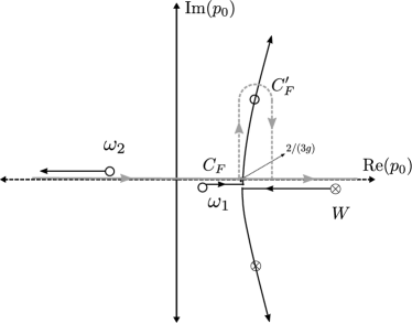
Figure 1: The path of integration $C_{F}$ when all the poles are real and the deformed path $C^{\prime}_{F}$ when $\omega_{1}$ and $W$ become complex.

The solutions (II) can be classified according to the sign of the discriminant $\Delta=E_{p}^{2}(2-\beta)$, which leads to the following three cases:

1. When $\Delta>0$, all solutions are real ($\beta<2$) and $\xi$ is a complex number that moves in the clockwise direction on a semicircle of unit norm, starting at the angle $\theta^{\prime}_{0}=gm\sqrt{27}$; see Fig. 2.

2. When $\Delta=0$, which we call the critical value ($\beta=2$), the two solutions $\omega_{1}$ and $W$ collapse at $\frac{2}{3g}$, and $\omega_{2}=-\frac{1}{3g}$, which may be seen using $\xi=1$ in Eq. (II).

3. When $\Delta<0$, the two solutions $\omega_{1}$ and $W$ become complex conjugate pairs, i.e., $\omega_{1}=W^{*}$ $(\beta>2)$, while the solution $\omega_{2}$ remains real. We have that $\xi$ is a real number larger than $1$, see Fig. 2.

In order to characterize the poles, let us consider the asymptotic expansion for the limit $g\to 0$

$$\omega_{1} = E_{p}+\frac{gE_{p}^{2}}{2}+\frac{5g^{2}E_{p}^{3}}{8}+\mathcal{O}(g^{3})\,,$$

$$\omega_{2} = -E_{p}+\frac{gE_{p}^{2}}{2}-\frac{5g^{2}E_{p}^{3}}{8}+\mathcal{O}(g^{3})\,,$$ (18)

$$W = \frac{1}{g}-gE_{p}^{2}-2g^{3}E_{p}^{4}+\mathcal{O}(g^{5})\,,$$

valid for $E_{p}\ll 1$. As usual, one can associate $\omega_{1}$ and $\omega_{2}$ to a particle and antiparticle, respectively, while $W$ to an additional particle which we call the Lee-Wick-like particle. In this sense, one may regard the higher time derivative theory with an indefinite metric as a Lee-Wick-like extension given that the poles $W$ and $\omega_{1}$ only become complex conjugate pairs in a certain range of energies, as we will see below.

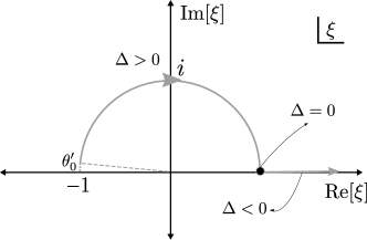
Figure 2: The energy function $\xi$ in terms of $\Delta$.

The Feynman propagator can be defined as

$$i\Delta(p_{0},\vec{p},\epsilon) = \frac{i}{(p_{0}-\omega_{1}+i\epsilon)(p_{0}-\omega_{2}-i\epsilon)}$$ (19)

$$\times \frac{1}{-g(p_{0}-W+i\epsilon)}\,,$$

with the negative pole $\omega_{2}$ located in the second quadrant and positive poles $\omega_{1}$ and $W$ in the fourth; see Fig. 1. That is, $\omega_{1}$ and $W$ ($\Delta>0$) lie below the path of integration $C_{F}$ and $\omega_{2}$ above. The poles $\omega_{1}$ and $W$ move in the opposite direction in the real axis collapsing at $\frac{2}{3g}$ ($\Delta=0$), while $\omega_{2}$ always moves to the left in the real axis. For energies ($\Delta<0$) the equivalent path $C^{\prime}_{F}$ rounds the complex solution $\omega_{1}$ from above. This prescription enjoys the desirable property to recover the standard position of the perturbative poles in the limit $g\to 0$ and to be connected to the Euclidean theory through a Wick rotation. In Fig. 1 the circles denote the perturbative poles and the encircled crosses the Lee-Wick-like pole.

The analysis for a lightlike four-vector $n=(1,0,0,1)$ is very similar to the previous case. By considering the dispersion relation

$$p_{0}^{2}-E_{p}^{2}-g(p_{0}-p_{3})^{3}=0\,,$$ (20)

the solutions are

$$\gamma_{1} = \frac{1}{3g}\left(1+3gp_{3}+(1+6gp_{3})\eta^{-1/3}z_{0}+\eta^{1/3}z_{0}^{*}\right)\,,$$

$$\gamma_{2} = \frac{1}{3g}\left(1+3gp_{3}-(1+6gp_{3})\eta^{-1/3}-\eta^{1/3}\right)\,,$$ (21)

$$\gamma_{3} = \frac{1}{3g}\left(1+3gp_{3}+(1+6gp_{3})\eta^{-1/3}z_{0}^{*}+\eta^{1/3}z_{0}\right)\,,$$

where again $z_{0}=e^{-\frac{i\pi}{3}}$ and we have defined the expressions

$$\eta = \frac{1}{2}\left(\delta+\sqrt{\delta^{2}-4(1+6gp_{3})}\right)\,,$$

$$\delta = -2+27g^{2}E_{p}^{2}-18gp_{3}-27g^{2}p_{3}^{2}\,.$$ (22)

As before, considering the limit $g\to 0$, we identify the solution $\gamma_{3}$ with the propagation of a Lee-Wick-like state.

III Perturbative unitarity

In this section we study perturbative unitarity at one-loop order for the graph shown in Fig. 3 by considering a purely timelike and spacelike preferred four-vector.

Figure 3: The forward scattering of a particle and antiparticle with momenta $p_{1}$ and $p_{2}$, respectively.

We write the loop amplitude

$$i\mathcal{M}(p) = (i\lambda)^{2}\int\frac{d^{4}q}{(2\pi)^{4}}\Delta(q_{0},\vec{q},\epsilon)\Delta(q_{0}-p_{0},\vec{q}-\vec{p},\epsilon)$$ (23)

in terms of a generic external momenta $p=(p_{0},\vec{p})$ such that $p=p_{1}+p_{2}$. Here energy flows through the cut towards the shaded region as shown in Fig 3.

III.1 Purely spacelike $n$

Consider a spacelike four-vector $n=(0,0,0,\vec{n})$ in the amplitude Eq. (23) and with the propagator (14)

$$i\mathcal{M}(p) = -\lambda^{2}\int\frac{d^{4}q}{(2\pi)^{4}}\frac{i}{(q_{0}-\omega_{s}+i\epsilon)(q_{0}+\omega_{s}-i\epsilon)}$$ (24)

$$\times \frac{i}{(q_{0}-p_{0}-\Omega_{s}+i\epsilon)(q_{0}-p_{0}+\Omega_{s}-i\epsilon)}\,.$$

The notation is

$$\Omega_{s} = \sqrt{(\vec{p}-\vec{q})^{2}+m^{2}-g(\vec{n}\cdot(\vec{p}-\vec{q}))^{3}}\,,$$ (25)

$$\omega_{s} = \sqrt{\vec{q}^{2}+m^{2}-g(\vec{n}\cdot\vec{p})^{3}}\,,$$ (26)

with the last term defined in Eq. (6).

The integration over $q_{0}$ is performed with the method of residues and we close the contour from below, enclosing the poles $\omega_{s}-i\epsilon$ and $p_{0}+\Omega_{s}-i\epsilon$. After summing the two contributions we have

$$i\mathcal{M}(p) = i\lambda^{2}\int\frac{d^{3}q}{(2\pi)^{3}}\frac{(\omega_{s}+\Omega_{s}-2i\epsilon)}{2(\omega_{s}-i\epsilon)(\Omega_{s}-i\epsilon)(\omega_{s}+\Omega_{s}-p_{0}-2i\epsilon)(\omega_{s}+\Omega_{s}+p_{0}-2i\epsilon)}\,.$$ (27)

Next, we set $\epsilon=0$, where it does not affect the computation of the discontinuity, which follows from the identity

$$\frac{1}{x\pm i\epsilon}=\mathcal{P}\left(\frac{1}{x}\right)\mp i\pi\delta(x)\,.$$ (28)

In this way we arrive at

$$\text{Disc}\mathcal{M}(p) = i\lambda^{2}\int\frac{d^{3}q}{(2\pi)^{3}}(2\pi)\left[\frac{\delta(p_{0}-\omega_{s}-\Omega_{s})}{4\omega_{s}\Omega_{s}}+\frac{\delta(p_{0}+\omega_{s}+\Omega_{s})}{4\omega_{s}\Omega_{s}}\right]\,.$$ (29)

We introduce the four-vectors $q_{1}=(q_{01},\vec{q})$ and $q_{2}=(q_{02},\vec{p}-\vec{q})$ with $q_{01}=\omega_{s}$ and $q_{02}=\Omega_{s}$. With this, we first rewrite

$$\text{Disc}\mathcal{M}(p) = i\lambda^{2}\int\frac{d^{3}q}{(2\pi)^{3}}(2\pi)\int dq_{01}\int dq_{02}\delta(p_{0}-q_{01}-q_{02})$$ (30)

$$\times \left[\frac{\delta(q_{01}-\omega_{s})\delta(q_{02}-\Omega_{s})}{4\omega_{s}\Omega_{s}}+\frac{\delta(q_{01}-\omega_{s})\delta(q_{02}-\Omega_{s})}{4\omega_{s}\Omega_{s}}\right]\,,$$

and then by using

$$\int\frac{d^{3}q}{(2\pi)^{3}}=\int\frac{d^{3}q_{1}}{(2\pi)^{3}}\int\frac{d^{3}q_{2}}{(2\pi)^{3}}(2\pi)^{3}\delta^{(3)}(\vec{p}-\vec{q}_{1}-\vec{q}_{2})\,,$$ (31)

we transform the integral into

$$\text{Disc}\mathcal{M}(p) = i\lambda^{2}\int\frac{d^{4}q_{1}}{(2\pi)^{4}}\int\frac{d^{4}q_{2}}{(2\pi)^{4}}(2\pi)^{4}\delta^{(4)}(p-q_{1}-q_{2})\left[\frac{(2\pi)\delta(q_{01}-\omega_{s})(2\pi)\delta(q_{02}-\Omega_{s})}{2\omega_{s}2\Omega_{s}}\right.$$ (32)

$$+ \left.\frac{(2\pi)\delta(q_{01}+\omega_{s})(2\pi)\delta(q_{02}+\Omega_{s})}{2\omega_{s}2\Omega_{s}}\right]\,.$$

Finally, using the identity $\text{Disc}\mathcal{M}=2i\text{Im}M$, we have

$$2\text{Im}\mathcal{M}(p) = \lambda^{2}\int\frac{d^{4}q_{1}}{(2\pi)^{4}}\int\frac{d^{4}q_{2}}{(2\pi)^{4}}(2\pi)^{4}\delta^{(4)}(p-q_{1}-q_{2})\delta(q_{1}^{2}-m^{2}-g(\vec{n}\cdot\vec{q}_{1})^{3})\delta(q_{2}^{2}-m^{2}-g(\vec{n}\cdot\vec{q}_{2})^{3})$$ (33)

$$\times \left[\theta(q_{01}\theta(q_{02}))+\theta(-q_{01})\theta(-q_{02})\right]\,.$$

From the cut diagram of the right, we identify the sum over intermediate states, the conservation of momenta coded in the first delta and the two propagators put on shell through the deltas of the dispersion relation. We may further simplify the result by considering the routing where energy flows with positive $q_{01}$ and $q_{02}$. Finally, we have that the optical theorem is satisfied in our process at the one-loop level.

III.2 Purely timelike $n$

From the previous sections, we have seen that a Lee-Wick-like particle arises when $n$ is chosen in the purely timelike direction. In order to study unitarity, we follow the Lee-Wick prescription in which only positive-norm states are regarded as stable, so removing from the asymptotic space the Lee-Wick-like particles Lee-Wick . The prescription is far from being trivial since Lee-Wick-like states may arise within the loops, spoiling any attempt to preserve unitarity. Hence, as a general statement one can say that if unitarity is to be conserved, no Lee-Wick-like states should propagate through the cut.

The amplitude is written with the propagator of Eq. (19)

$$i\mathcal{M}(p) = \lambda^{2}\int\frac{d^{4}{q}}{(2\pi)^{4}}\prod_{i=1}^{2}\frac{1}{(q_{0}^{(i)}-\omega_{1}^{(i)}+i\epsilon)(q_{0}^{(i)}-{\omega_{2}^{(i)}}-i\epsilon)}$$ (34)

$$\times \frac{1}{-g(q_{0}^{(i)}-W^{(i)}+i\epsilon)}\,,$$

and with the new notation where $q_{0}^{(1)}=q_{0}$ and $q_{0}^{(2)}=q_{0}-p_{0}$, together with

$$\omega_{1}^{(1)} = \omega_{1}(\vec{q})\,,\qquad\omega_{1}^{(2)}=\omega_{1}(\vec{p}-\vec{q})\,,$$

$$\omega_{2}^{(1)} = \omega_{2}(\vec{q})\,,\qquad\omega_{2}^{(2)}=\omega_{2}(\vec{p}-\vec{q})\,,$$

$$W^{(1)} = W(\vec{q})\,,\qquad W^{(2)}=W(\vec{p}-\vec{q}).$$ (35)

The first propagator has poles at

$$\alpha_{1} = \omega_{1}(\vec{q})-i\epsilon\,,$$

$$\alpha_{2} = \omega_{2}(\vec{q})+i\epsilon\,,$$

$$\alpha_{3} = W(\vec{q})-i\epsilon\,,$$ (36)

and the second propagator, which depends on the external momenta, has poles at

$$\beta_{1} = p_{0}+\omega_{1}(\vec{q}-\vec{p})-i\epsilon\,,$$

$$\beta_{2} = p_{0}+\omega_{2}(\vec{q}-\vec{p})+i\epsilon\,,$$

$$\beta_{3} = p_{0}+W(\vec{q}-\vec{p})-i\epsilon\,,$$ (37)

they are depicted in Fig. 4.

Let us perform the integral in $q_{0}$ using the residue theorem and closing the contour of $q_{0}$ in the lower half plane. In this way, we enclose the poles $\alpha_{1}$, $\alpha_{3}$, $\beta_{1}$, and $\beta_{3}$ to obtain

$$i\mathcal{M}(p) = -i\lambda^{2}\int\frac{d^{3}{\vec{q}}}{(2\pi)^{3}}\Big{(}\text{Res}(\alpha_{1})+\text{Res}(\alpha_{3})$$ (38)

$$+ \text{Res}(\beta_{1})+\text{Res}(\beta_{3})\Big{)}\,,$$

where the corresponding residues are

$$\text{Res}(\alpha_{1}) = \frac{1}{g^{2}(\alpha_{1}-\alpha_{2})(\alpha_{1}-\alpha_{3})(\alpha_{1}-\beta_{1})}$$

$$\times \frac{1}{(\alpha_{1}-\beta_{2})(\alpha_{1}-\beta_{3})}\,,$$

$$\text{Res}(\alpha_{3}) = \frac{1}{g^{2}(\alpha_{3}-\alpha_{1})(\alpha_{3}-\alpha_{2})(\alpha_{3}-\beta_{1})}$$

$$\times \frac{1}{(\alpha_{3}-\beta_{2})(\alpha_{3}-\beta_{3})}\,,$$

$$\text{Res}(\beta_{1}) = \frac{1}{g^{2}(\beta_{1}-\alpha_{1})(\beta_{1}-\alpha_{2})(\beta_{1}-\alpha_{3})}$$

$$\times \frac{1}{(\beta_{1}-\beta_{2})(\beta_{1}-\beta_{3})}\,,$$

$$\text{Res}(\beta_{3}) = \frac{1}{g^{2}(\beta_{3}-\alpha_{1})(\beta_{3}-\alpha_{2})(\beta_{3}-\alpha_{3})}$$ (39)

$$\times \frac{1}{(\beta_{3}-\beta_{1})(\beta_{3}-\beta_{2})}\,.$$

For the expressions above involving a $\beta$, where a $p_{0}$ appears, we consider the $\epsilon$ dependence and we compute the discontinuity using the expression

$$\frac{1}{x\pm i\epsilon}=\mathcal{P}\left(\frac{1}{x}\right)\mp i\pi\delta(x)\,,$$ (40)

where $\mathcal{P}$ denotes the principal value. For the other terms we just evaluate $\epsilon$ to zero. Adding all the residues gives

$$\text{Disc}\left(\sum Res\right)=-\frac{2\pi i}{g^{2}}$$ (41)

$$\times \Big{(}\frac{\delta(p_{0}-\omega_{2}+\mkern 1.5mu\overline{\mkern-1.5mu\omega\mkern-1.5mu}\mkern 1.5mu_{1})}{(\omega_{1}-\omega_{2})(\mkern 1.5mu\overline{\mkern-1.5mu\omega\mkern-1.5mu}\mkern 1.5mu_{1}-\mkern 1.5mu\overline{\mkern-1.5mu\omega\mkern-1.5mu}\mkern 1.5mu_{2})(\omega_{2}-W)(\mkern 1.5mu\overline{\mkern-1.5mu\omega\mkern-1.5mu}\mkern 1.5mu_{1}-\mkern 1.5mu\overline{\mkern-1.5muW\mkern-1.5mu}\mkern 1.5mu)}$$

$$+ \frac{\delta(p_{0}-\omega_{1}+\mkern 1.5mu\overline{\mkern-1.5mu\omega\mkern-1.5mu}\mkern 1.5mu_{2})}{(\omega_{1}-\omega_{2})(\mkern 1.5mu\overline{\mkern-1.5mu\omega\mkern-1.5mu}\mkern 1.5mu_{1}-\mkern 1.5mu\overline{\mkern-1.5mu\omega\mkern-1.5mu}\mkern 1.5mu_{2})(\omega_{1}-W)(\mkern 1.5mu\overline{\mkern-1.5mu\omega\mkern-1.5mu}\mkern 1.5mu_{2}-\mkern 1.5mu\overline{\mkern-1.5muW\mkern-1.5mu}\mkern 1.5mu)}$$

$$+ \frac{\delta(p_{0}+\mkern 1.5mu\overline{\mkern-1.5mu\omega\mkern-1.5mu}\mkern 1.5mu_{2}-W)}{(\mkern 1.5mu\overline{\mkern-1.5mu\omega\mkern-1.5mu}\mkern 1.5mu_{1}-\mkern 1.5mu\overline{\mkern-1.5mu\omega\mkern-1.5mu}\mkern 1.5mu_{2})(\omega_{1}-W)(\omega_{2}-W)(\mkern 1.5mu\overline{\mkern-1.5mu\omega\mkern-1.5mu}\mkern 1.5mu_{2}-\mkern 1.5mu\overline{\mkern-1.5muW\mkern-1.5mu}\mkern 1.5mu)}$$

$$+ \frac{\delta(p_{0}-\omega_{2}+\mkern 1.5mu\overline{\mkern-1.5muW\mkern-1.5mu}\mkern 1.5mu)}{(\omega_{1}-\omega_{2})(\omega_{2}-W)(\mkern 1.5mu\overline{\mkern-1.5mu\omega\mkern-1.5mu}\mkern 1.5mu_{1}-\mkern 1.5mu\overline{\mkern-1.5muW\mkern-1.5mu}\mkern 1.5mu)(\mkern 1.5mu\overline{\mkern-1.5mu\omega\mkern-1.5mu}\mkern 1.5mu_{2}-\mkern 1.5mu\overline{\mkern-1.5muW\mkern-1.5mu}\mkern 1.5mu)}\Big{)}\,,$$

where the notation is $\mkern 1.5mu\overline{\mkern-1.5muX\mkern-1.5mu}\mkern 1.5mu=X(\vec{p}-\vec{q})$.

Organizing the terms and recalling that we are taking the energy flow in one direction where $p_{0}$ is positive, we drop the first and fourth contribution to arrive at

$$2\text{Im}\mathcal{M} = \lambda^{2}\int\frac{d^{3}{\vec{q}}}{(2\pi)^{3}}\frac{2\pi}{g^{2}}\left(\frac{\delta(p_{0}-\omega_{1}+\mkern 1.5mu\overline{\mkern-1.5mu\omega\mkern-1.5mu}\mkern 1.5mu_{2})}{(\omega_{1}-\omega_{2})(\mkern 1.5mu\overline{\mkern-1.5mu\omega\mkern-1.5mu}\mkern 1.5mu_{1}-\mkern 1.5mu\overline{\mkern-1.5mu\omega\mkern-1.5mu}\mkern 1.5mu_{2})(\omega_{1}-W)}\right.$$ (42)

$$\times \left.\frac{1}{(\mkern 1.5mu\overline{\mkern-1.5mu\omega\mkern-1.5mu}\mkern 1.5mu_{2}-\mkern 1.5mu\overline{\mkern-1.5muW\mkern-1.5mu}\mkern 1.5mu)}+\frac{\delta(p_{0}+\mkern 1.5mu\overline{\mkern-1.5mu\omega\mkern-1.5mu}\mkern 1.5mu_{2}-W)}{(\mkern 1.5mu\overline{\mkern-1.5mu\omega\mkern-1.5mu}\mkern 1.5mu_{1}-\mkern 1.5mu\overline{\mkern-1.5mu\omega\mkern-1.5mu}\mkern 1.5mu_{2})(\omega_{1}-W)(\omega_{2}-W)}\right.$$

$$\times \left.\frac{1}{(\mkern 1.5mu\overline{\mkern-1.5mu\omega\mkern-1.5mu}\mkern 1.5mu_{2}-\mkern 1.5mu\overline{\mkern-1.5muW\mkern-1.5mu}\mkern 1.5mu)}\right)\,,$$

where we have used the identity $\text{Disc}\mathcal{M}=2i\text{Im}\mathcal{M}$.

The second delta is nonvanishing when the pole $\alpha_{3}$ of the first propagator collapses with the pole $\beta_{2}$ of the second propagator, as can be seen in Fig. 4. In this case both poles pinch the path of integration. It is not difficult to show that no other pinching occurs, since the pole $\alpha_{2}$ has opposite sign compared to all other poles and eventually never hits any of them.

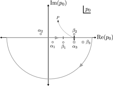
Figure 4: The relevant poles $\alpha_{1}$, $\beta_{1}$, $\alpha_{3}$, $\beta_{3}$ and the pinching point $P$ for the collapse of $\beta_{2}$ and $\alpha_{3}$ on the contour of integration.

In order to analyze the pinching condition $\beta_{2}=\alpha_{3}$, we consider $\xi=e^{i\theta}$ with the angle $\theta=\tan^{-1}\left(\frac{\sqrt{4-\beta^{2}}}{\beta}\right)$ defined in the interval $0<\theta<\pi$.

Using these expressions in Eqs. (II) yields

$$\omega_{1} = \frac{1}{3g}\left(1+\cos\frac{\theta}{3}-\sqrt{3}\sin\frac{\theta}{3}\right)\,,$$

$$\omega_{2} = \frac{1}{3g}\left(1-2\cos\frac{\theta}{3}\right)\,,$$

$$W = \frac{1}{3g}\left(1+\cos\frac{\theta}{3}+\sqrt{3}\sin\frac{\theta}{3}\right)\,.$$ (43)

We begin with the case where the external space momenta vanish, i.e., $\vec{p}=0$. In this reference frame (center of mass frame), we arrive at

$$3gp_{0}=3\cos\frac{\theta}{3}+\sqrt{3}\sin\frac{\theta}{3}\,,$$ (44)

which has the solution

$$\theta_{0}=\frac{\pi}{2}\pm 3\cos^{-1}\left(\frac{\sqrt{3}gp_{0}}{2}\right)\,,$$ (45)

for $1/g<p_{0}<2/\sqrt{3}g$. Taking the threshold to be $p_{0}=1/g$, we have that the pinching occurs at $\theta=0$ ($\Delta=0$) which lies outside the interval of $\theta$. In this way it is enough to take $p_{0}<1/g$ to avoid the propagation of nonphysical degrees of freedom.

Let us consider the case $\vec{p}\neq 0$. It can be shown that a variation in the energy is equivalent to an increment of the angle $\theta$, which we denote by $\delta\theta$. According to Eqs. (II) and (II), an increment in the momenta is equivalent to an increment of second order $\delta\theta\sim g^{2}$. The new equation at which we arrive is

$$3gp_{0}=3a\cos\frac{\theta}{3}+\sqrt{3}b\sin\frac{\theta}{3}\,,$$ (46)

where

$$a=\frac{1}{3}\left(1+2\cos\left(\frac{\delta\theta}{3}\right)\right)\,,$$ (47)

and

$$b=1-\frac{2}{\sqrt{3}}\sin\left(\frac{\delta\theta}{3}\right)\,.$$ (48)

It can be seen that, at lowest order in $g$, we arrive at the same result we have obtained for Eq. (44). In addition, in the region in which $\Delta<0$, we have complex solutions and so there is no contribution to the discontinuity.

Finally, the relevant contribution is

$$2\text{Im}\mathcal{M} = \lambda^{2}\int\frac{d^{3}{\vec{q}}}{(2\pi)^{3}}\frac{2\pi}{g^{2}}$$ (49)

$$\times \frac{\delta(p_{0}-\omega_{1}+\mkern 1.5mu\overline{\mkern-1.5mu\omega\mkern-1.5mu}\mkern 1.5mu_{2})}{(\omega_{1}-\omega_{2})(\omega_{1}-W)(\mkern 1.5mu\overline{\mkern-1.5mu\omega\mkern-1.5mu}\mkern 1.5mu_{1}-\mkern 1.5mu\overline{\mkern-1.5mu\omega\mkern-1.5mu}\mkern 1.5mu_{2})(\mkern 1.5mu\overline{\mkern-1.5mu\omega\mkern-1.5mu}\mkern 1.5mu_{2}-\mkern 1.5mu\overline{\mkern-1.5muW\mkern-1.5mu}\mkern 1.5mu)}\,.$$

Let us define $k_{1}=q$ and $k_{2}=q-p$, together with $\omega_{1}^{\prime}=\omega_{1}(\vec{k}_{1})$, $\omega_{2}^{\prime}=\omega_{2}(\vec{k}_{1})$, $\omega_{1}^{\prime\prime}=\omega_{1}(\vec{k}_{2})$ and $\omega_{2}^{\prime\prime}=\omega_{2}(\vec{k}_{2})$, and write

$$2\text{Im}\mathcal{M}=\lambda^{2}\int\frac{d^{4}{k_{1}}}{(2\pi)^{4}}\int\frac{d^{4}{k_{2}}}{(2\pi)^{4}}(2\pi)^{4}\delta^{(4)}(p-k_{1}+k_{2})$$ (50)

$$\times \left(\frac{(2\pi)^{2}\delta(k^{0}_{1}-\omega_{1}^{\prime})\delta(k^{0}_{2}-\omega_{2}^{\prime\prime})}{g(k^{0}_{1}-\omega^{\prime}_{2})(W^{\prime}-k^{0}_{1})g(\omega_{1}^{\prime\prime}-k^{0}_{2})(W^{\prime\prime}-k^{0}_{2})}\right)\,.$$

At this point, it is convenient to define a physical delta

$$\delta^{(\text{phys})}(p^{2}-m^{2}-gp_{0}^{3})=\sum_{\text{phys},a}\frac{\delta(p_{0}-p_{a})}{|F^{\prime}(p_{a})|}\,,$$ (51)

where $p_{a}$ are the zeros of the function $F(p_{0})=p_{0}^{2}-E_{\vec{p}}^{2}-gp_{0}^{3}$ and where we have to exclude the contribution from the Lee-Wick-like pole. Considering

$$\delta^{(\text{phys})}(k_{1}^{2}-m^{2}-gk_{01}^{3})\theta(k_{1}^{0}) = \frac{\delta(k^{0}_{1}-\omega_{1})\theta(k_{1}^{0})}{g(k^{0}_{1}-\omega_{2})(W-k^{0}_{1})}\,,$$

$$\delta^{(\text{phys})}(k_{2}^{2}-m^{2}-gk_{02}^{3})\theta(-k_{2}^{0}) = \frac{\delta(k^{0}_{2}-\omega_{2})\theta(-k_{2}^{0})}{g(\omega_{1}-k^{0}_{2})(W-k^{0}_{2})}\,,$$

where we have used the absolute value in the definition of Eq. (51), we rewrite

$$2\text{Im}\mathcal{M}=\lambda^{2}\int\frac{d^{4}{k_{1}}}{(2\pi)^{4}}\int\frac{d^{4}{k_{2}}}{(2\pi)^{4}}(2\pi)^{4}\delta^{(4)}(p-k_{1}+k_{2})$$ (53)

$$\times (2\pi)^{2}\delta^{(\text{phys})}(k_{1}^{2}-m^{2}-gk_{01}^{3})\delta^{(\text{phys})}(k_{2}^{2}-m^{2}-gk_{02}^{3})$$

$$\times \theta(k_{1}^{0})\theta(-k_{2}^{0})\,.$$

In this way we arrive at the phase space sum of the cut diagram, hence, proving the unitarity constraint in our diagram and one-loop unitarity in our theory.

We note that as in the usual case, one could have replaced the propagators with the physical deltas in the cut diagrams

$$\frac{i}{-g(p_{0}-\omega_{1}+i\varepsilon)(p_{0}-\omega_{2}-i\varepsilon)(p_{0}-W+i\varepsilon)}$$

$$\to 2\pi\delta^{(\text{phys})}(k_{1}^{2}-m^{2}-gk_{01}^{3})\theta(k_{1}^{0})\,,$$ (54)

and

$$\frac{i}{-g(q_{0}-p_{0}-\omega_{1}+i\varepsilon)(q_{0}-p_{0}-\omega_{2}-i\varepsilon)(q_{0}-p_{0}-W+i\varepsilon)}$$

$$\to\delta^{(\text{phys})}(k_{2}^{2}-m^{2}-gk_{02}^{3})\theta(-k_{2}^{0})\,,$$ (55)

simplifying the analysis from the beginning and being of potential utility in other models.

IV Conclusions

In this work we have focused on the Myers-Pospelov effective field theory with dimension-five Lorentz violating operators in order to study one-loop unitarity. In the first part, we have studied the solutions of the dispersion relation for purely spacelike, timelike and lightlike backgrounds. We have found that when $n$ is purely spacelike, one has two perturbative solutions which become complex when momenta are higher than $\mathcal{P}$. In addition, we have found that possible issues regarding the canonical quantization may arise in highly boosted frames due to spacelike solutions of the dispersion relation. In the spacelike case, without Lee-Wick particles, we have directly verified the optical theorem at one-loop level. For the the timelike case, we have found two perturbative poles which in the limit $g\to 0$ tend to the standard ones, and in accordance with the higher time derivative character of the theory, an additional pole corresponding to a particle with negative norm. The poles have been characterized according to the sign of the discriminant and we have found that above the critical energy $\frac{2}{g\sqrt{27}}$ the two poles $\omega_{1}$ and $W$ become complex and move as complex conjugate pairs, while $\omega_{2}$ always remains in the real axis. In this way, we have determined the evolution of the three poles in the complex energy plane. The lightlike case is very similar to the timelike case and presents no new ingredients.

The main part of this investigation has been to study whether it is possible to preserve unitarity by applying the Lee-Wick prescription, which requires us to excise the Lee-Wick-like particles from the physical Hilbert space. In particular, we have analyzed the forward scattering of antiparticle-particle annihilation with a quartic interaction term. We have studied the bubble diagram with the optical theorem and computed the possible contributions to the discontinuity. It has been found that the Lee-Wick-like pole contributes to the discontinuity provided a pinching singularity takes place or equivalently when the path of integration passes between two infinitely close poles. Performing a detailed analysis one can show that for real external momenta the pinching condition cannot be fulfilled and so its contribution vanishes.

Finally, by comparing with the cut diagram where we identify the sum over intermediate states, conservation of momenta, and on-shell contributions of the propagators, we have verified unitarity at the one-loop level. In addition, we have shown that an alternative and more direct route may be supplied with a physical delta defined to select only poles associated to stable particles. In other words, we have shown the equivalence of replacing the propagators on shell with physical deltas in the cut diagrams. It may be part of future work to study whether this feature is maintained in other Lorentz violating models.

References

• (1) V. A. Kostelecky and S. Samuel, Phys. Rev.  D 39, 683 (1989); V. A. Kostelecky and R. Potting, Nucl. Phys.  B 359, 545 (1991); R. Gambini and J. Pullin, Phys. Rev. D 59, 124021 (1999); J. Alfaro, H. A. Morales-Tecotl and L. F. Urrutia, Phys. Rev. Lett.  84, 2318 (2000); S. M. Carroll, J. A. Harvey, V. A. Kostelecky, C. D. Lane and T. Okamoto, Phys. Rev. Lett.  87, 141601 (2001).
• (2) D. Colladay and V. A. Kostelecky, Phys. Rev. D 55, 6760 (1997); D. Colladay and V. A. Kostelecky, Phys. Rev. D 58, 116002 (1998).
• (3) V. A. Kostelecky and M. Mewes, Phys. Rev. D 80, 015020 (2009); A. Kostelecky and M. Mewes, Phys. Rev. D 85, 096005 (2012); A. Kosteleck and M. Mewes, Phys. Rev. D 88, no. 9, 096006 (2013).
• (4) R. C. Myers and M. Pospelov, Phys. Rev. Lett.  90 (2003) 211601.
• (5) L. Maccione, S. Liberati, A. Celotti and J. G. Kirk, JCAP 0710, (2007) 013; L. Maccione and S. Liberati, JCAP 0808, (2008) 027.
• (6) R. Montemayor and L. F. Urrutia, Phys. Rev.  D 72, 045018 (2005); R. Montemayor and L. F. Urrutia, Phys. Lett. B 606 (2005) 86.
• (7) V. A. Kostelecky and N. Russell, Rev. Mod. Phys.  83, 11 (2011).
• (8) R. Casana, M.M. Ferreira, R.V. Maluf, and F.E.P. dos Santos, Phys. Rev. D 86, 125033 (2012); R. Casana, M.M. Ferreira, Jr., E.O. Silva, E. Passos, and F.E.P. dos Santos, Phys. Rev. D 87, 047701 (2013); J.B. Araujo, R. Casana and M.M. Ferreira, Phys. Rev. D 92, 025049 (2015); L. H. C. Borges, A. F. Ferrari and F. A. Barone, Eur. Phys. J. C 76, no. 11, 599 (2016).
• (9) C. M. Reyes, L. F. Urrutia and J. D. Vergara, Phys. Rev.  D 78, 125011 (2008); C. M. Reyes, L. F. Urrutia and J. D. Vergara, Phys. Lett.  B 675, 336 (2009).
• (10) T. Mariz, Phys. Rev. D 83, 045018 (2011); T. Mariz, J. R. Nascimento and A. Y. .Petrov, Phys. Rev. D 85, 125003 (2012); J. Leite, T. Mariz and W. Serafim, J. Phys. G 40, 075003 (2013); T. Mariz, J. R. Nascimento, A. Y. Petrov and H. Belich, J. Phys. Communications 1, 045011 (2017).
• (11) A. Pais and G. E. Uhlenbeck, Phys. Rev.  79, 145 (1950).
• (12) T. D. Lee and G. C. Wick, Nucl. Phys. B 9, 209 (1969); T. D. Lee, G. C. Wick, Phys. Rev.  D2, 1033-1048 (1970).
• (13) R. E. Cutkosky, P. V. Landshoff, D. I. Olive and J. C. Polkinghorne, Nucl. Phys. B 12, 281 (1969).
• (14) B. Grinstein, D. O’Connell and M. B. Wise, Phys. Rev. D 77, 025012 (2008); J. R. Espinosa, B. Grinstein, D. O’Connell and M. B. Wise, Phys. Rev. D 77, 085002 (2008); J. R. Espinosa and B. Grinstein, Phys. Rev. D 83, 075019 (2011).
• (15) D. Anselmi, JHEP 1802, 141 (2018); D. Anselmi and M. Piva, JHEP 1706, 066 (2017); D. Anselmi and M. Piva, Phys. Rev. D 96, no. 4, 045009 (2017).
• (16) C. M. Reyes and L. F. Urrutia, Phys. Rev. D 95, no. 1, 015024 (2017); M. Maniatis and C. M. Reyes, Phys. Rev. D 89, no. 5, 056009 (2014); C. M. Reyes, Phys. Rev. D 87, no. 12, 125028 (2013); J. Lopez-Sarrion and C. M. Reyes, Eur. Phys. J. C 73, no. 4, 2391 (2013).
• (17) M. Schreck, Phys. Rev. D89, no. 10, 105019 (2014); M. Schreck, Phys. Rev. D90, no. 8, 085025 (2014).
• (18) R. Potting, Phys. Rev. D85, 045033 (2012).
• (19) M. Cambiaso, R. Lehnert and R. Potting, Phys. Rev. D90, 065003 (2014); M. Cambiaso, R. Lehnert and R. Potting, Phys. Rev. D 85, 085023 (2012).
• (20) J. R. Nascimento, A. Y. Petrov and C. M. Reyes, Eur. Phys. J. C 78, no. 7, 541 (2018); C. M. Reyes, S. Ossandon and C. Reyes, Phys. Lett. B 746, 190 (2015).
• (21) V. A. Kostelecky and R. Lehnert, Phys. Rev. D 63, 065008 (2001).
• (22) D. Colladay, J. Phys. Conf. Ser.  952, no. 1, 012011 (2018); D. Colladay, P. McDonald, J. P. Noordmans and R. Potting, Phys. Rev. D 95, no. 2, 025025 (2017); D. Colladay, Phys. Lett. B 772, 694 (2017).