A Binary Offset Effect in CCD Readout and its Impact on Astronomical Data

Abstract

We have discovered an anomalous behavior of CCD readout electronics that affects their use in many astronomical applications. An offset in the digitization of the CCD output voltage that depends on the binary encoding of one pixel is added to pixels that are read out one, two and/or three pixels later. One result of this effect is the introduction of a differential offset in the background when comparing regions with and without flux from science targets. Conventional data reduction methods do not correct for this offset. We find this effect in 16 of 22 instruments investigated, covering a variety of telescopes and many different front-end electronics systems. The affected instruments include LRIS and DEIMOS on the Keck telescopes, WFC3-UVIS and STIS on HST, MegaCam on CFHT, SNIFS on the UH88 telescope, GMOS on the Gemini telescopes, HSC on Subaru, and FORS on VLT. The amplitude of the introduced offset is up to 4.5 ADU per pixel, and it is not directly proportional to the measured ADU level. We have developed a model that can be used to detect this "binary offset effect" in data and correct for it. Understanding how data are affected and applying a correction for the effect is essential for precise astronomical measurements.

1 Introduction

Charge coupled devices (CCDs) have been the dominant astronomical detector for the past three decades. Ideally, light at the focal plane of the telescope is detected on a grid of pixels which each provide independent information about the incident light at their location. In practice, astronomical CCDs and the associated instruments are subject to many anomalies that introduce spurious signals, correlations between pixels or deviation from linear behavior. These anomalies will lead to errors in the derived scientific results if they are not understood and accounted for. There are several locations in the instrument where such anomalies can be introduced.

Many of the anomalies are related to imperfections in the production of the sensor. These include variations in the pixel areas, fringing due to variations in thickness of the CCD, "tree ring" patterns due to impurities in the production of the silicon wafers, manufacturing defects in the CCD electronics, and edge effects due to interactions with other components or guard rings. See Janesick (2001) or Stubbs (2014) for in-depth discussions of these effects. Localized contamination of the silicon can also lead to many undesirable effects, including hot pixels with high dark current and traps that interfere with the charge transfer of pixels read out later in the same column. Large traps can produce dead or hot columns, while smaller traps lead to charge transfer inefficiency (CTI). Baggett et al. (2012) discusses localized contamination in the HST WFC3 UVIS detectors and studies how it evolves with time.

Several anomalies arise due to normal instrument operations even with a defect-free CCD. For very bright sources, the CCD can saturate, leading to effects such as blooming where charge spills into neighboring pixels. In general, the presence of charge on the CCD distorts the nearby electric field. This distortion manifests itself as effects like the "brighter-fatter effect" where the widths of point-spread functions vary by up to 2% for bright and faint objects (Antilogus et al., 2014). It is also possible to accumulate charge on the CCD from sources other than the desired science target, such as cosmic rays which deposit charge as they pass through the CCD (Janesick, 2001), or optical reflections ("ghosts") that appear when light reflects in unintended ways off of external optical components such as filters (Brown & Lupie, 2004) or within the CCD itself.

Readout electronics can introduce another set of anomalies. Many readout systems are susceptible to pickup that appears as periodic oscillations in the measured values of pixels that are observed sequentially. This can introduce a herring-bone pattern across the CCD image (Jansen et al., 2003). Other potential artifacts of the readout electronics include undershooting after reading a bright pixel (Caldwell et al., 2010), crosstalk between the readouts from different amplifiers (Baggett et al., 2004), and biased/sticky bits in analog-to-digital converters (Robberto & Hilbert, 2005). Understanding how all of these effects interact with scientific data is essential for proper calibration of the science output of an instrument. Techniques have been developed to correct for most of these effects, and data reduction pipelines typically endeavor to treat the ones that have a sizeable effect on the data taken by their targeted instrument.

In this paper, we report a newly discovered CCD electronic chain artifact which originates in the readout electronics of many commonly-used CCD electronics systems. We find that there is crosstalk between the binary-coded output of the analog-to-digital converter (ADC) and subsequently read-out pixels. An offset is introduced into the subsequently read-out pixels which is roughly proportional to the number of "1" bits in the binary encoding of a driver pixel. This effect is present in a wide variety of currently-used instruments with different electronics configurations. We have characterized the effect and modeled it with high accuracy in the SuperNova Integral Field Spectrograph (SNIFS; Lantz et al., 2004) instrument used by the Nearby Supernova Factory collaboration (SNfactory; Aldering et al., 2002) on the UH88 telescope. We call this CCD-electronics-chain artifact the "binary offset effect".

We proceed as follows. In Section 2 we discuss how to identify this effect in CCD data. In Section 3, we build a model of the effect which can predict the size of the introduced offsets given the adjacent pixel values, and we provide an example of data corrected with this model. In Section 4, we then discuss how scientific results can be impacted by this effect if it is not corrected for.

2 Identifying the Binary Offset Effect

2.1 Evidence of the Binary Offset Effect in SNIFS Data

The binary offset effect was first observed in data taken with SNIFS for the SNfactory (Lantz et al., 2004; Aldering et al., 2002). SNIFS contains two lenslet integral field unit (IFU) spectrographs which produce spectra over a 15$\times$15 grid of spatial elements (spaxels). The spectrographs simultaneously cover wavelength ranges of 3200-5200 Å and 5100-10000 Å for the blue and red channels respectively. Each spectrograph uses a CCD composed of 2048$\times$4096 15 micron pixels. The blue channel uses a thinned E2V model 44-82 CCD while the red channel uses a thinned and deep depleted E2V CCD44-82-0-A72 CCD. These CCDs are of the highest scientific grade. Each CCD is read out by two independent amplifiers using an Astronomical Research Cameras (ARC) Generation II video board (Leach et al., 1998).

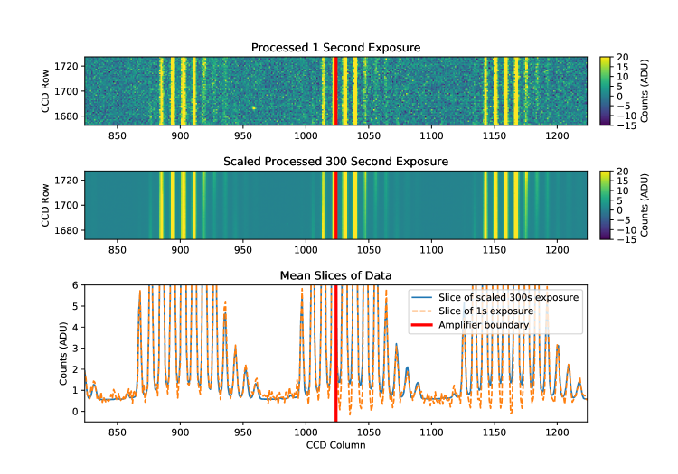
Figure 1: Comparison of 1 and 300 second dome flat exposures with the SNIFS instrument. Top panel: 1 second exposure. Middle panel: 300 second exposure. The vertical lines (which saturate the scale) are the traces of spectra for each of the individual spaxels. The amplifier boundary on the CCD is indicated with a vertical red line. Bottom panel: slices through the previous images showing the mean values of the pixels in each CCD column with CCD row values between 1400 and 2000. The 300 second exposure has been scaled by its exposure time to match the 1 second exposure. On the right amplifier, there is a deficit in the measured counts between each spaxel for the 1 second exposure relative to the 300 second exposure, although the background regions are in agreement. These large deficits are not present on the left amplifier.

The binary offset effect can be easily seen by looking at images where there is an accurate model of the light on the CCD, and by probing the residuals after this model is subtracted from the data. Here, we examine a set of 1 second dome flat exposures taken with SNIFS. We take a 300 second exposure in the same configuration, and we treat this exposure as a model of the true light on the CCD because this exposure has high count levels compared to the size of the effects that we are looking into. An example of these dome flat CCD exposures is shown in Figure 1, where the spectral traces due to the IFU reformatting of the dome flat are all visible. We systematically work with the output of the CCD in analog-to-digital units (ADU) throughout this paper. The top two panels of Figure 1 show examples of the dome flat exposures after applying an overscan subtraction, a bias correction, and a dark correction. The bottom panel of this figure shows slices through both one of the 1 second dome flat exposures and the 300 second exposure scaled to match the exposure time of the 1 second exposure. On the right amplifier, there is a count deficit of 1-2 ADU in between each of the spaxels on the 1 second exposure relative to the 300 second one. This same deficit is not seen on the left amplifier.

To probe the cause this deficit, we subtract a scaled version of the 300 second exposure (which we use here as our reference model) from each of the 1 second exposures to obtain residual images. For each 1 second exposure, we then compare the residual values of each pixel after the model was subtracted to the raw value (number of ADU) measured in a pixel that was read out 2 pixels earlier. We call the pixel read out 2 pixels earlier the "driver pixel". We take the mean of all residuals that have the same driver pixel value, and we plot the mean residual as a function of the driver pixel value. The results of this procedure are shown in Figure 2.

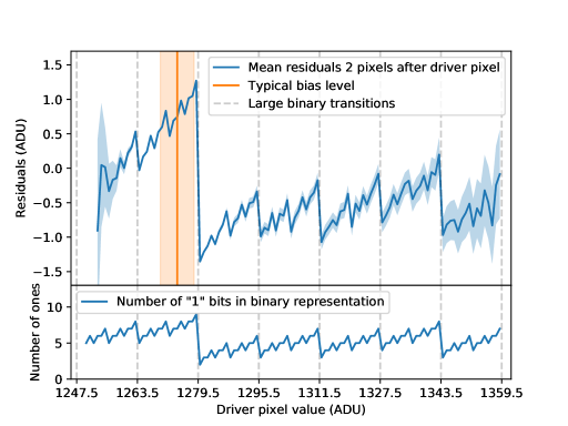
Figure 2: Example of the binary offset effect on the SNIFS blue channel right amplifier. See text for details on how this plot was produced. Top panel: mean residuals as a function of the raw driver pixel value read out 2 pixels earlier along with an uncertainty band. Bottom panel: number of "1" bits in the binary representation of the driver pixel value. We label transitions where more than 5 bits flip with a vertical dashed line. All of the features in the bottom panel, including the large transitions, are visible in the residual data. The mean background level and one standard deviation of read noise are illustrated with a vertical orange line and surrounding band.

The resulting plot gives a very jagged function: a single ADU difference in the driver pixel value can correspond to a difference of up to 2.5 ADU in the mean of the residuals of the pixel read out 2 pixels afterwards. These differences are highly statistically significant; the measurement uncertainties are less than 0.05 ADU between driver pixel values of 1260 and 1290. A careful analysis of these large differences reveals that they map out the number of "1" bits in the binary representation of the driver pixel value. For example, Figure 2 shows that there is a difference of 2.5 ADU when transitioning from a driver pixel value of 1279 ADU to a driver pixel value of 1280 ADU. The binary representations of these two numbers are 100 1111 1111 and 101 0000 0000 respectively. Other large differences occur between 1311 ADU and 1312 ADU (101 0001 1111 and 101 0010 0000) and between 1343 ADU and 1344 ADU (101 0011 1111 and 101 0100 0000). The lower panel of Figure 2 shows the plot of the number of "1" bits in the binary representation of the driver pixel for comparison. All of the features in this plot are seen in the residual data, from the large binary transitions down to odd-even effects.

Figure 3 shows the same residuals from Figure 2 plotted directly against the number of "1" bits in the binary representation of the driver pixel value. There is a linear trend between the mean of the residuals and the number of "1" bits in the binary representation of the driver pixel value. This is consistent with this effect being mostly related to the total number of "1" bits rather than it being due to some issue with the uppermost bits. There is an offset in the zeropoint of this linear relation for values below 1280 ADU indicating that a linear model with the number of "1" bits is not a complete description of the effect. In Section 3 we will discuss how to properly model this effect.

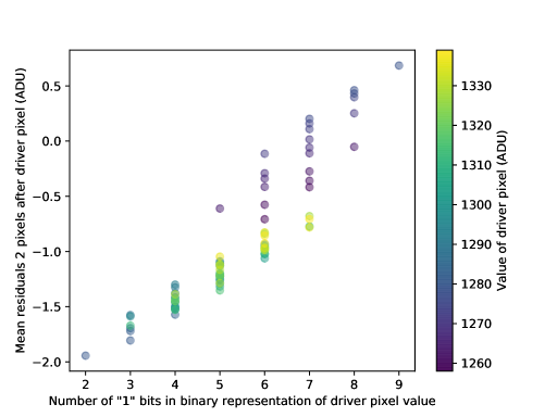
Figure 3: Example of the binary offset effect on the SNIFS blue channel right amplifier. This plot shows the same data as in Figure 2 with a cut requiring that the uncertainty on the mean of the residuals be less the 0.2 ADU. Instead of plotting the mean of the residuals directly against the driver pixel values as in Figure 2, we sum the number of "1" bits in the binary representation of each driver pixel value in ADU, and we plot the mean of the residuals against this number. There is a clear linear trend in the mean of the residuals with the number of "1" bits in the binary representation, at all scales. It is also apparent that there are some additional effects, such as an offset in the zeropoint of the linear relation near a driver pixel value of 1280 ADU.

2.2 Implications of the Binary Offset Effect in SNIFS Data

The binary offset effect introduces a highly non-linear signal into images taken with the CCD. The main consequence of the binary offset effect is that an offset can be introduced to CCD data that only appears in regions where sufficient flux from science targets is present on the CCD. To show how this appears in data, we examine stacks of face-on cosmic rays in dark exposures taken with the SNIFS instrument. An example of such a stack is shown in Figure 4. These images were originally taken in effort to measure the in-situ CTI of the SNIFS instrument (Dixon et al., 2016), and a small CTI tail can be seen on the upper part of the image. We also find a deficit in the measured count levels of pixels read out 2-3 pixels after a cosmic ray compared to the background level. We find that the size of the deficit varies from night to night, from no effect up to around 1 ADU per pixel. The size of the deficit is not the same on each amplifier. This deficit is the result of the binary offset effect, and it can be thought of as an offset that is added to the data when the count levels of previous pixels cross a specific threshold. The deficit has a roughly fixed count value that does not scale with the amount of flux in the preceding pixels, so it does not behave as a simple modification to the PSF. The binary offset effect hence effectively introduces a deficit wherever there is sufficient flux from science targets on the CCD, leading to a local offset in the measured count values for regions on the CCD with flux from science targets compared to those without any flux.

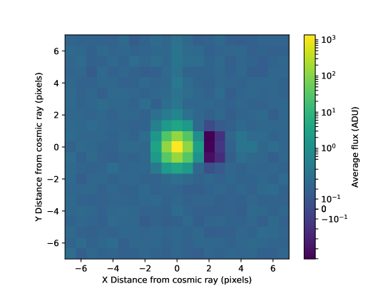
Figure 4: Stacked cosmic ray frames from the right amplifier of the SNIFS blue channel. This image was generated by taking a series of dark exposures on a night, identifying all face-on cosmic rays in the image, and taking the clipped mean of all pixels around cosmic rays. The color scale on this plot changes from linear to logarithmic at 0.5 ADU in order to capture the full dynamic range of the image. The serial readout reads pixels from left to right in this image. There is a visible deficit of $\sim$0.5 ADU 2-3 pixels following the cosmic ray.

An explanation of how the binary offset effect can cause such a deficit can be seen from Figure 2. The raw background level (before overscan subtraction) on the dome flat images used to generate this figure is around 1274 ADU with 4.5 ADU (or 3 electrons) of read noise per unstacked pixel. This background level is illustrated with an orange line and surrounding band on the figure. Most background pixels are therefore below the threshold of 1280 ADU, where there is a large change in the binary representation of the driver pixel value. When there is at least a small amount of signal on the CCD, the pixel values are brought above the 1280 ADU threshold and a $\sim$2 ADU offset is introduced into subsequently read pixels compared to the background regions. The consequences of the binary offset effect for a science image can be seen in the lower panel of Figure 1: for the right amplifier, a deficit appears in the 1 second dome flat exposure compared to the 300 second exposure wherever the average count levels are above a few counts. On the left amplifier, the bias level is at 1285 ADU, and there are no major binary transitions in the nearby higher count levels. The binary offset effect is still present, but introduced offsets are similar for all pixels so no major difference is observed between background and science regions.

When extracting the spectra from images affected by the binary offset effect, the introduced offsets will propagate to the extracted spectra. The two amplifiers will, in general, have different bias levels, so they will be affected in different ways by the binary offset effect. Hence, systematic differences will be observed in spectra extracted from each of the two amplifiers. The SNfactory collaboration discovered these systematic differences before the cause was known, and dubbed this effect the "blue step" as it was primarily noticed at the bluest wavelengths where the expected fluxes of SNIFS’s primary objects of interest (Type Ia supernovae) can be faint. To illustrate the blue step, we extract spectra for each of the IFU spaxels in one of the 1 second dome flat exposures using the standard SNfactory pipeline (Aldering et al., 2006; Scalzo et al., 2010), and we calculate the average flux in the 4000 to 4500 Å region. The results of this procedure are shown in Figure 5. We find a 2.2 ADU difference in the measured counts between the two amplifiers, corresponding to a 4.2% difference in the measured fluxes between the two amplifiers for this exposure. The observed difference is well-modeled by a flat difference in the background level between the different amplifiers, as expected for a signal introduced in the previously described manner. The average offset introduced by the binary offset is different in regions on the CCD with and without flux present, meaning that there is a effectively a pathological local background offset that only appears where there is flux on the CCD. Conventional background subtraction routines cannot identify or correct for the difference in background levels introduced by the binary offset effect because these methods measure the background level in locations on the CCD where there is no flux present.

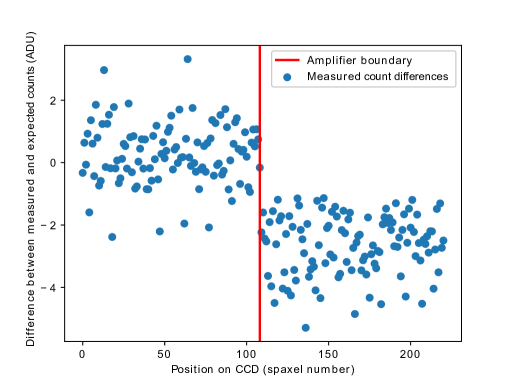
Figure 5: Exposure-time normalized difference between extracted 1 second and 300 second dome flats from the SNIFS blue channel, illustrating the "blue step". Each point corresponds to the average flux of a spaxel in the 4000 to 4500 Å region. We indicate the boundary where the readout switches from the left to the right amplifier with a vertical red line. We find a 2.2 ADU difference in the measured fluxes between the two amplifiers which corresponds to a 4.2% difference in the measured flux for this example.

2.3 Cause of the Binary Offset Effect

The discussion up to this point has shown that an offset is introduced into pixels that are read out two pixels after the driver pixel. We find a similar offset three pixels after the driver pixel for each CCD amplifier on both the blue and red SNIFS channels. There is no effect 1 pixel after or 4 or more pixels after, nor is there an offset for pixels before the driver pixel. The ARC video board used by SNIFS processes pixels one at a time, so the timeframe of 2-3 pixels between the driver and affected pixels implies that there must be some feedback in the electronics chain from somewhere after the ADC conversion. We varied the gain of the SNIFS front-end electronics by a factor of 10, and we find that the amplitude of the effect is constant in ADU. This implies that the introduction of the feedback must occur past the gain electronics in the CCD electronics chain. We also notice that the binary offset effect shows up across amplifiers: a driver pixel will introduce an offset in the pixels that are read out 3 pixels later in the other amplifier with a similar amplitude to the offset introduced on the driver pixel’s amplifier.

Combining all of these findings, we propose that the binary offset effect is being caused by feedback into the reference voltage of the ADC. The ADC is highly sensitive to small changes in its reference voltages: one ADU for a 16-bit ADC corresponds to a change of only 0.0015%. When earlier pixels are read out, the ADC outputs their binary representations and stores them temporarily. We propose that these charges (representing the ones in the binary code) then introduce a slight offset into the reference voltage when they are released and the next pixel is read out.

2.4 The Binary Offset Effect in Other Instruments

We wrote a program that can identify the binary offset effect in CCD data from any telescope by looking for the characteristic saw-tooth shape in the mean of the residuals as a function of the driver pixel value seen in Figure 2. We find that the effect is present in most astronomical instruments that are currently in use across a variety of different readout systems. As we are not able to build a model using different length exposures of our own on all of these instruments, we use bias or dark images to probe the effect, and we assume that the pixel values in these images can be modeled by a smooth function. We fit for such a model using the background determined by sep (Barbary, 2016; Bertin & Arnouts, 1996) with $64\times 64$ pixel boxes. We subtract this model from the original images to obtain residual images. With dark and bias images, we are limited to probing the effect over a smaller baseline of driver values (typically around 10 ADU). We are, however, able to achieve very high signal-to-noise by averaging the residuals over the full image and by examining multiple images. We estimate the amplitude of the binary offset effect by measuring the largest difference in residuals between two adjacent driver pixel values. For the SNIFS images shown in Figure 2, this corresponds to the size of the transition from 1279 to 1280. We note that the measurement uncertainties on the stacked residuals are around 0.01 ADU for most instruments, so this method is sensitive to effects larger than $\sim$0.05 ADU. The results are summarized in Table 1.

We are able to detect the binary offset effect in 16 of 22 instruments that were investigated. The amplitude of the offset varies significantly between the different instruments. We provide a Jupyter notebook (Kluyver et al., 2016) that contains code to probe this effect for all of the instruments listed in Table 1. This Jupyter notebook is available on GitHub at https://github.com/snfactory/binaryoffset. Plots of the binary offset effect are shown for a representative sample of the different instruments in Figure 6.

Table 1: Size of the binary offset effect in different instruments. See text and accompanying Jupyter notebook for details on how these measurements were made. We have attempted to determine the CCD electronics front end and ADC wherever possible for comparison purposes.

Telescope	Instrument	Distance from	Approximate peak-to-peak	Amplitude in	CCD front end	ADC	Reference
		driver pixel to	amplitude of binary	electrons
		target pixel (pixels)	offset effect (ADU)
Blanco	DECam	-	Not detected (< 0.05)	Not detected (< 0.2)	Monsoon	Analog Devices AD7674	Castilla et al. (2010)
CFHT	Megacam	1	0.4	0.6		Linear Technology LTC 1604	de Kat et al. (2004)
Gemini	GMOS-S E2V	2, 3	0.7	1.4	ARC Gen. II	Datel ADS-937	Hook et al. (2004)
	GMOS-S Hamamatsu	-	Not detected (< 0.05)	Not detected (< 0.08)	ARC Gen. III		Gimeno et al. (2016)
	GMOS-N E2V	2, 3	0.7	1.4	ARC Gen. II	Datel ADS-937	Hook et al. (2004)
	GMOS-N Hamamatsu	-	Not detected (< 0.05)	Not detected (< 0.09)	ARC Gen. III		Gimeno et al. (2016)
HST	WFC3 UVIS	1	0.05-0.15a	0.08-0.23a
	STIS (post SM4)	1	0.5-4.5a	0.5-4.5a
	ACS	1, 2, 3, 4	0.4-1.0a	0.4-1.0a
Keck	DEIMOS	2	2.6	3.2	ARC Gen. II	Datel ADS-937	Wright et al. (2003)
	HIRES	2	0.3	0.6	ARC Gen. I	Datel ADS-937	Kibrick et al. (1993)
	LRIS B	2	0.15	0.24	ARC Gen. I	Datel ADS-937	McCarthy et al. (1998)
	LRIS R (upgraded)	2	0.15	0.15	ARC Gen. II	Datel ADS-937	Rockosi et al. (2010)
SDSS	-	-	Not detected (< 0.05)	Not detected (< 0.23)		Crystal Semiconductor CS5101A	Gunn et al. (1998)
Subaru	Suprime-Cam	-	Not detected (< 0.05)	Not detected (< 0.15)	MFront	Analogic ADC423	Miyazaki et al. (2002)
	Hyper Suprime-Cam	1	0.5b	1.6b	MFront2	Analog Devices AD7686C	Nakaya et al. (2012)
	FOCAS	2	0.1b	0.2b	MFront	Analogic ADC423	Kashikawa et al. (2002)
UH88	SNIFS blue channel	2, 3	2.4	1.8	ARC-41 Gen. II	Datel ADS-937	Aldering et al. (2002)
	SNIFS red channel	2, 3	1.5	1.1	ARC-41 Gen. II	Datel ADS-937	Aldering et al. (2002)
VLT	FORS 1	1	0.1	0.22	FIERA	Analogic ADC4320Ac	Beletic et al. (1998)
	FORS 2	1	0.1	0.13	FIERA	Analogic ADC4320Ac	Beletic et al. (1998)
	MUSE	-	Not detected (< 0.05)	Not detected (< 0.06)	NGC	Analog Devices AD7677c	Reiss et al. (2012)

• ^a For the labeled HST instruments, there is a strong trend in the mean of the residuals with the least-significant bit (odd-even) along with large offsets when higher bits change. Intermediate bits do not appear to have any effect.

• ^b In Subaru Hyper Suprime-Cam and FOCAS images we find a trend in the mean of the residuals with the least-significant bit (odd-even). The higher bits do not appear to have a direct impact on the mean of the residuals.

• ^c We thank J. Reyes (ESO) for details of the ADCs used in the VLT instruments. (personal communication, August 2017)

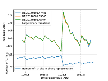
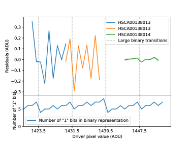
(a) DEIMOS (Keck), 2 pixels after the driver pixel.	(b) Hyper Suprime-Cam (Subaru), 1 pixel after
The median measurement uncertainty for the	the driver pixel. The median measurement
residuals is 0.012 ADU.	uncertainty for the residuals is 0.006 ADU.
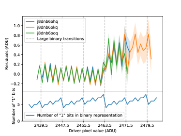
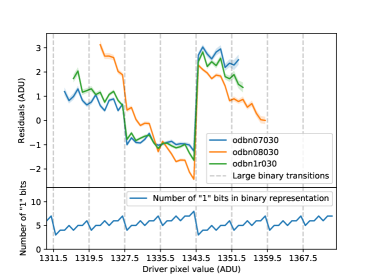
(c) ACS (HST), 1 pixel after the driver pixel.	(d) STIS (HST), 1 pixel after the driver pixel.
The median measurement uncertainty for the	The median measurement uncertainty for the
residuals is 0.030 ADU.	residuals is 0.077 ADU.

Figure 6: Examples of the binary offset effect in other instruments. For half of the instruments that were investigated, such as DEIMOS on Keck, we see an effect that has similar properties to the effect on SNIFS. For other instruments, such as Hyper Suprime-Cam on Subaru, ACS on HST, or STIS on HST, we find evidence of offsets related to the binary representation, but the offsets have a different dependence on the binary encoding. All plots are shown with their measurement uncertainties as a shaded contour, and the median measurement uncertainty is given in the subpanel caption. These measurement uncertainties are very small compared to the size of the observed effects, and all of these observed effects are highly statistically significant. The specific observations used to generate each plot are listed in the figure legends.

For all of the detections in Table 1 from instruments on the CFHT, Gemini, Keck, UH88 and VLT telescopes (11 of the 22 instruments investigated), we see an offset in the mean of the residuals that is roughly proportional to the number of "1" bits in the binary representation of the driver pixel, similar to what is seen for SNIFS. The amplitude of the effect varies significantly between instruments, from a peak-to-peak amplitude of approximately 0.1 ADU for FORS 2 on VLT to a peak-to-peak amplitude of approximately 2.6 ADU for DEIMOS on Keck (see Figure 6a). We also find that the number of pixels following the driver pixel at which the binary offset effect appears varies from 1 to 3 pixels for the different instruments. All of the instruments tested using ARC Generation I or II controllers (Leach et al., 1998) show this kind of binary offset effect, although the size of the effect varies from instrument to instrument. The newer ARC Generation III controllers used in GMOS-S and GMOS-N do not show any evidence of the binary offset effect.

In the images from Hyper Suprime-Cam (HSC) on Subaru, we find offsets in the mean of the residuals, but they do not appear to be linearly related to the number of "1" bits in the binary encoding of the driver pixel value (see Figure 6b). The mean of the residuals shows peak-to-peak offsets of 0.5 ADU between adjacent driver pixel values with a median measurement uncertainty of 0.006 ADU, so the detection of an offset related to the driver pixel value is highly significant. There appears to be a correlation of the least-significant bit (i.e. whether the driver pixel value is even or odd) with the mean of the residuals. Unlike the previously-described instruments, large changes in the binary representation do not appear to correlate with large offsets in the mean of the residuals. The introduced offsets do still have a highly nonlinear and nonmonotonic dependence on the driver pixel values, although additional work is needed to understand these offsets. For images taken with the FOCAS instrument on Subaru we see a similar effect, although the amplitude is smaller.

Images from all of the HST instruments that were examined (WFC3 UVIS, STIS and ACS) show evidence of an effect related to the binary encoding of driver pixels but with somewhat different behavior. An example of the effect in ACS is shown in Figure 6c. The least-significant bit (odd-even) has a large effect on the mean of the residuals, but transitions of the next several bits do not appear to have a significant impact. However, when the sixth bit or higher is changed, a step is introduced into the mean of the residuals. For the ACS images shown in Figure 6c, we see an offset of 0.4 ADU at the transition from 2463 ADU to 2464 ADU (1001 1001 1111 to 1001 1010 0000).

The STIS instrument on HST displays a similar behavior to ACS. An example of the binary offset effect on STIS is shown in Figure 6d. For STIS, when the fifth bit or higher is changed, we notice a large offset, but there is little effect for the less significant bits. At the transition from 1343 ADU to 1344 ADU (101 0011 1111 to 101 0100 0000) there is a 4.5 ADU offset in the mean of the residuals. We find that the size of the offsets when the upper bits are changed varies dramatically, from 0.5 ADU up to the offset of 4.5 ADU previously mentioned.

For several instruments, the binary offset effect introduces artifacts that are large compared to the size of the signals being observed. On SNIFS, the blue step was identified and characterized before it was understood as being a result of the binary offset effect. It is likely that the consequences of the binary offset effect have been identified in other instruments without the root cause being fully understood.

3 Modeling and Correcting the Offset for Active Instruments

The binary offset effect is present in a large fraction of existing CCD data, as illustrated by Table 1, and correcting for the effect will both improve the quality of existing data and allow previously unusable data to be recovered. As a working example of such a correction, we have derived a model that can calculate the introduced offsets in SNIFS data.

As illustrated in Figure 3, the amplitude of the effect is primarily proportional to the number of "1" bits in the binary encoding of the driver pixel. However, this figure illustrates that the effect is not simply a linear function of the driver pixel value, as the zeropoint of the linear relation appears to shift when the driver pixel values drop below 1280 ADU. These details of the effect are second order, but must be taken into account to generate an accurate model. We have developed a 9-parameter model which can capture the behavior of the binary offset effect in SNIFS data. We trained this model on a set of bias images covering the full history of SNIFS operations (2004-2017). The details of this model can be found in the Appendix.

We find that this single set of model parameters is able to describe the behavior of an amplifier over the entire history of the SNIFS instrument. That is; the model parameters do not vary over time, and a single set of parameters per amplifier is sufficient to cover the full range of observed temperatures, bias levels and signal levels. The behavior of the binary offset effect does vary significantly between amplifiers, and we therefore use a unique set of model parameters for each amplifier. This is consistent with the idea that the digitization is the root cause, since each amplifier has its own video board. With this model, we are able to predict the amplitude of the offsets introduced by the binary offset effect to within 0.11-0.16 ADU depending on the amplifier. We can predict the amplitudes of the offsets for every pixel in an image, and we can use these predictions to build a correction image which can be subtracted from the data to remove the binary offset effect. Applying this procedure to a new image only requires the raw pixel counts of the image and a set of previously-derived model parameters for that amplifier. No additional fitting is required.

As a test of the model, we applied the derived correction to the set of 1 and 300 second dome flat exposures described in Section 2.1. The results of this procedure can be seen in Figure 7. The dome flat images were not included the dataset on which the model was trained, so this is an out-of-sample test of the model. The deficits seen on the right amplifier in the slice plot of Figure 1 are no longer present after correction. We applied the same algorithm used to produce Figure 2 to the corrected data. The results of this procedure are shown in Figure 8. As seen from this figure, the offsets introduced by the binary offset effect are effectively removed from the data when the correction is applied. The remaining linear slope in the residuals is a consequence of the high frequency pickup described in the Appendix, and is not a feature of the binary offset effect.

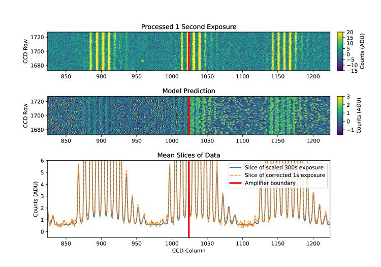
Figure 7: Results of the binary offset effect model for the SNIFS image shown in Figure 1. Top panel: original 1 second exposure. Middle panel: model prediction of the signal introduced by the binary offset effect. Bottom panel: slices through the previous images showing the mean values of the pixels in each CCD column with CCD row values between 1400 and 2000. For the right amplifier, the model predicts that the binary offset effect introduces an offset of $\sim$2 ADU ($\sim$1.3 electrons) at the specific locations on the CCD where spectral traces are found relative to the background locations. When these corrections are applied to the data, the count deficits seen in Figure 1 for the slice of the 1 second exposure on the right amplifier are eliminated.

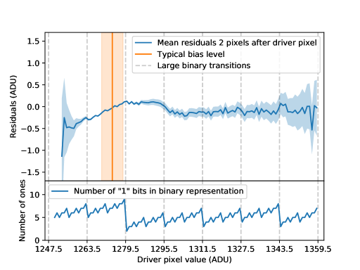
Figure 8: Example of data that previously exhibited the binary offset effect on the SNIFS blue channel right amplifier, after correcting for the effect. See Figure 2 for the same data before correction and an explanation of how this figure was produced. The residuals after correction no longer have a strong dependence on the binary encoding. There is a slight linear slope in the residuals for driver pixel values between $\sim$1250-1280 ADU; this slope arises due to correlations introduced by high frequency pickup, as discussed in the Appendix, and is not related to the binary offset effect.

4 Impact of the Binary Offset Effect on Scientific Results

4.1 Impact of the Binary Offset Effect on SNIFS/SNfactory Data

The binary offset effect introduces a highly non-linear signal into CCD data that affects science results in several ways. As discussed in Section 2.2, for the SNIFS instrument, the binary offset effect can introduce an offset to the data that only appears at locations on the CCD with a significant amount of flux. This can be seen directly in the model in Figure 7: on the right amplifier, there is a visible offset of $\sim$2 ADU ($\sim$1.3 electrons) at the specific locations on the CCD where spectral traces are found relative to the background regions. The model predicts that the binary offset effect has little impact on the left amplifier due to the bias level being above the large binary transition at 1280.

We subtract the derived model from one of the 1 second dome flat exposures, and we extract the spectra in the corrected image using the SNfactory pipeline. The result of this procedure is shown in Figure 9, which can be compared to Figure 5 on the same data before corrections. The previous offset of 2.2 ADU has been removed and we constrain the corrected offset between the amplifiers to be less than 0.2 ADU (0.13 electrons), confirming that the binary offset effect was the cause of the "blue step" in this data and that our model is capable of removing it.

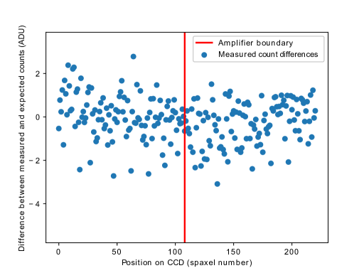
Figure 9: Corrected exposure-time normalized difference between extracted 1 second and 300 second dome flats from the SNIFS blue channel. See Figure 5 for details and comparison. We find that the offsets between the two amplifiers are consistent to within 0.2 ADU (0.13 electrons) after correction.

We apply the binary offset correction to a series of SNfactory observations of Type Ia supernovae that are representative of the range of measured flux levels on the CCD for scientific observations. We find that the blue channel is the most strongly affected by the binary offset effect. For the full dataset, the NMAD (normalized median absolute deviation) of the applied corrections ranges is 0.04 mag at UV wavelengths and 0.02 mag for blue (B-band) wavelengths, while if we look at the faintest 20th percentile of data ordered by flux level, we find that the corrections in UV have a much larger NMAD of 0.51 mag and those in the blue have an NMAD of 0.11 mag. Corrections on the red channel have an NMAD of less than 0.008 mag over the full dataset, and an NMAD of less than 0.05 mag for the faintest 20 percent of observations. The binary offset correction is therefore relatively small for the majority of the dataset, but it has a disproportionately high impact on fainter regions of our spectra on the blue channel.

The affected spectra in SNfactory data are typically at late phases of the supernova lightcurves where the intrinsic supernova flux is low. In practice, however, the SNfactory collaboration had previously developed methods to identify spectra affected by the binary offset effect (before recognizing the cause), primarily by looking for anomalous behavior in the UV, where it stands out. These spectra were not included in previous published analyses. Although the corrections for the binary offset thus should not affect any previous results, we do expect that it will allow future analyses to include many spectra that were previously rejected, especially spectra at late phases.

4.2 Impact of the Binary Offset Effect on General Astronomical Data

There are several science scenarios where the binary offset effect can have large impacts on science data. The conditions that lead to the largest potential impact are:

• Low background noise.

• Low signal levels.

• A background level just below a large binary transition.

Low-flux observations with fiber-fed, lenslet, or similar spectrographs are very susceptible to this effect. In these cases, most of the CCD is not in the path of any light, so the background in those regions is entirely dominated by read noise. For modern instruments, this means that the background noise will be very low, on the order of a few ADU or less. When measuring the background level on the CCD with conventional methods, one will effectively sample the binary offset curve at the given bias level instead of measuring what the background truly is under the science data due to the small range of pixel values covered in the region used to measure the background level. Observations with ground-based slit spectrographs may be highly susceptible by the binary offset effect, although their susceptibility depends on how they are used. Observations of faint emission lines with low sky background or target continuum will be affected for the same reasons as fiber-fed and IFU spectrographs. As the binary offset effect introduces an offset that is shifted by 1-3 pixel from the data that it is applied to, the recovered wavelengths of emission lines may be biased. Higher resolution spectrographs are likely to be more strongly affected because of the reduction in sky background per pixel leading to low background noise levels on the CCD.

Science applications using ground-based CCD imaging are not as susceptible as spectrographs to the binary offset effect. Measurements of faint targets with these detectors are often limited by the sky background, so the potential size of the offset is suppressed. Imaging applications that have low backgrounds and low signals (for example U-band observations, narrow band imaging, imaging of standard stars, or very short exposures) are more likely to be affected. An additional issue for imaging is that the local background offset will have the same shape as the science signal, but will be shifted by 1-3 pixels depending on the instrument. This can affect measurements of the shape of a galaxy and may be a concern for some weak lensing analyses. The binary offset effect will also introduce some correlations between nearby pixels on the CCD.

Science applications using detectors in space-based missions are highly susceptible to the binary offset effect, regardless of whether they are being used as an imager or any type of spectrograph. For these instruments, the sky noise is often low compared to the readout noise so conventional background subtraction routines will effectively sample from a point on the binary offset curve rather than averaging over it. The STIS spectrograph on HST is of particular interest. We find an offset of up to 4.5 ADU for some binary transitions in this instrument. This offset is per pixel, so it can easily add up to a significant fraction of the science signal.

5 Conclusions

We have discovered an anomalous behavior in the read-out of CCDs: the introduction of spurious counts into a pixel, with an amplitude that depends on the binary encoding of a pixel read out 1-3 pixels previously. One consequence of this effect is that it can introduce a local background offset that only appears where sufficient flux from science targets is present on the CCD. This background offset is not removed by conventional background subtraction procedures. In SNIFS data, the effect can cause an offset in the final measured fluxes of up to 2 ADU per pixel. The binary offset effect explains several effects previously noticed in SNIFS data, notably the "blue step" where there is a flat offset between data from different amplifiers, and a fixed count deficit in pixels following cosmic rays. We find evidence of the binary offset effect in 16 of 22 different instruments that were investigated, indicating that the effect is present in a significant amount of existing astronomical data.

In this paper, we built a model that can predict, and thus reliably correct, the offsets introduced by this effect in affected CCD data, and we applied this model to SNIFS data. We find that the model parameters are stable in time, but that they are unique to the readout electronics of each amplifier. With this model, we can predict the amplitudes of the introduced offsets, and we use these predictions to correct for the binary offset effect. The model derived in this paper is general, and a variant of it should be applicable to any instrument. Because of the relatively large amplitudes of the introduced offsets relative to the noise levels, only a single bias image is typically required to characterize the effect and fit the model.

The binary offset effect can also be mitigated in hardware. Reducing opportunities for stray signals to affect the input of the ADC, e.g. using a differential input, should eliminate the binary offset effect. We find that 6 of the 22 instruments that we investigated do not show signs of this effect, as shown in Table 1. These can serve as a guide to design new readout electronics that aren’t susceptible to the binary offset effect. The size of the binary offset effect should be measured and characterized in any new CCD readout system to determine whether or not it will impact the science results. For systems where modifying the readout electronics is not practical, the bias level can at least be set to a level where there are no large binary transitions immediately above said bias level. This will minimize the potential size of the offsets although it will not eliminate them. Finally, the tests outlined in this paper should be performed for any CCD-based instrument likely to exhibit the binary offset effect, and the correction procedure that we present in this paper should be incorporated in the data-reduction pipeline of all instruments where the binary offset effect is found.

6 Acknowledgements

We thank the technical staff of the University of Hawaii 2.2 m telescope, and Dan Birchall for observing assistance. The authors wish to recognize and acknowledge the very significant cultural role and reverence that the summit of Maunakea has always had within the indigenous Hawaiian community. We are most fortunate to have the opportunity to conduct observations from this mountain. This work was supported in part by the Director, Office of Science, Office of High Energy Physics of the U.S. Department of Energy under Contract No. DE-AC02-05CH11231. Support in France was provided by CNRS/IN2P3, CNRS/INSU, and PNC; LPNHE acknowledges support from LABEX ILP, supported by French state funds managed by the ANR within the Investissements d’Avenir programme under reference ANR-11-IDEX-0004-02. Some results were obtained using resources and support from the National Energy Research Scientific Computing Center, supported by the Director, Office of Science, Office of Advanced Scientific Computing Research of the U.S. Department of Energy under Contract No. DE-AC02- 05CH11231. We thank the Gordon & Betty Moore Foundation for their continuing support. We also thank the High Performance Research and Education Network (HPWREN), supported by National Science Foundation Grant Nos. 0087344 & 0426879.

Funding for SDSS-III has been provided by the Alfred P. Sloan Foundation, the Participating Institutions, the National Science Foundation, and the U.S. Department of Energy Office of Science. The SDSS-III web site is http://www.sdss3.org/. SDSS-III is managed by the Astrophysical Research Consortium for the Participating Institutions of the SDSS-III Collaboration including the University of Arizona, the Brazilian Participation Group, Brookhaven National Laboratory, Carnegie Mellon University, University of Florida, the French Participation Group, the German Participation Group, Harvard University, the Instituto de Astrofisica de Canarias, the Michigan State/Notre Dame/JINA Participation Group, Johns Hopkins University, Lawrence Berkeley National Laboratory, Max Planck Institute for Astrophysics, Max Planck Institute for Extraterrestrial Physics, New Mexico State University, New York University, Ohio State University, Pennsylvania State University, University of Portsmouth, Princeton University, the Spanish Participation Group, University of Tokyo, University of Utah, Vanderbilt University, University of Virginia, University of Washington, and Yale University.

This project used public archival data from the Dark Energy Survey (DES). Funding for the DES Projects has been provided by the U.S. Department of Energy, the U.S. National Science Foundation, the Ministry of Science and Education of Spain, the Science and Technology Facilities Council of the United Kingdom, the Higher Education Funding Council for England, the National Center for Supercomputing Applications at the University of Illinois at Urbana-Champaign, the Kavli Institute of Cosmological Physics at the University of Chicago, the Center for Cosmology and Astro-Particle Physics at the Ohio State University, the Mitchell Institute for Fundamental Physics and Astronomy at Texas A&M University, Financiadora de Estudos e Projetos, Fundação Carlos Chagas Filho de Amparo à Pesquisa do Estado do Rio de Janeiro, Conselho Nacional de Desenvolvimento Científico e Tecnológico and the Ministério da Ciência, Tecnologia e Inovação, the Deutsche Forschungsgemeinschaft and the Collaborating Institutions in the Dark Energy Survey. The Collaborating Institutions are Argonne National Laboratory, the University of California at Santa Cruz, the University of Cambridge, Centro de Investigaciones Enérgeticas, Medioambientales y Tecnológicas-Madrid, the University of Chicago, University College London, the DES-Brazil Consortium, the University of Edinburgh, the Eidgenössische Technische Hochschule (ETH) Zürich, Fermi National Accelerator Laboratory, the University of Illinois at Urbana-Champaign, the Institut de Ciències de l’Espai (IEEC/CSIC), the Institut de Física d’Altes Energies, Lawrence Berkeley National Laboratory, the Ludwig-Maximilians Universität München and the associated Excellence Cluster Universe, the University of Michigan, the National Optical Astronomy Observatory, the University of Nottingham, the Ohio State University, the University of Pennsylvania, the University of Portsmouth, SLAC National Accelerator Laboratory, Stanford University, the University of Sussex, and Texas A&M University. Based in part on observations at Cerro Tololo Inter-American Observatory, National Optical Astronomy Observatory (NOAO Prop. I D and PI), which is operated by the Association of Universities for Research in Astronomy (AURA) under a cooperative agreement with the National Science Foundation.

Based in part on observations obtained with MegaPrime/MegaCam, a joint project of CFHT and CEA/DAPNIA, at the Canada-France-Hawaii Telescope (CFHT) which is operated by the National Research Council (NRC) of Canada, the Institut National des Sciences de l’Univers of the Centre National de la Recherche Scientifique (CNRS) of France, and the University of Hawaii.

Based in part on observations obtained at the Gemini Observatory acquired through the Gemini Observatory Archive, which is operated by the Association of Universities for Research in Astronomy, Inc., under a cooperative agreement with the NSF on behalf of the Gemini partnership: the National Science Foundation (United States), the National Research Council (Canada), CONICYT (Chile), Ministerio de Ciencia, Tecnología e Innovación Productiva (Argentina), and Ministério da Ciência, Tecnologia e Inovação (Brazil).

Based in part on observations made with the NASA/ESA Hubble Space Telescope, obtained from the Data Archive at the Space Telescope Science Institute, which is operated by the Association of Universities for Research in Astronomy, Inc., under NASA contract NAS 5-26555. These observations are associated with programs 9583, 13677, 14327, and 14820.

Some of the data presented herein were obtained at the W. M. Keck Observatory, which is operated as a scientific partnership among the California Institute of Technology, the University of California and the National Aeronautics and Space Administration. The Observatory was made possible by the generous financial support of the W. M. Keck Foundation. This research has made use of the Keck Observatory Archive (KOA), which is operated by the W. M. Keck Observatory and the NASA Exoplanet Science Institute (NExScI), under contract with the National Aeronautics and Space Administration.

Based in part on data collected at Subaru Telescope, which is operated by the National Astronomical Observatory of Japan.

Based in part on data obtained from the ESO Science Archive Facility under requests numbered kboone301279, kboone301093, and kboone301092.

Appendix A Modeling the Binary Offset Effect in SNIFS Data

In SNIFS data, we notice that an offset is introduced into the affected pixel related to the binary encodings of the driver pixels read out 2 and 3 pixels earlier. In the following discussion, we refer to a pixel that is affected by the binary offset as the "target". Each pixel on the CCD serves as a driver pixel for several other pixels. We subtract a model of the counts on the CCD from the measured data to obtain a residual image, and we compare the value of the residual image for each pixel to the raw ADU measured on the corresponding driver pixels. We refer to driver pixels that were read out N pixels before the target pixel as T-N. There is also some crosstalk between the amplifiers: the value of the pixel that was read out 3 pixels earlier in time on the other amplifier also affects the introduced offsets. We note that the timing of the readout of the other amplifier is what matters rather than the physical location on the CCD. We refer to driver pixels that were read out N pixels before the target pixel on the other amplifier as O-N.

We find that the binary codes of the driver pixels interact with each other in a complex way to produce the offset that is applied to the target pixel. There is a baseline linear trend of the introduced offsets with the number of "1" bits in pixels T-2 and T-3. However, there is also some interaction between these pixels: a bit in pixel T-2 behaves differently if that same bit was on in pixel T-3 compared to if it was off. The largest offsets occur when a bit is "1" in both T-2 and T-3. For pixel T-2, we find that the more significant bits have a larger effect on the introduced offset than the less significant bits. For pixel T-3, we find evidence of interactions across amplifiers: turning a bit from "0" to "1" in T-3 introduces an offset that depends on how many bits were already on in T-3 and in O-3. We model this interaction with a second order polynomial in the number of bits that are "1" in each of T-3 and O-3. We do not find any evidence of direct interactions across bits (e.g.: bit 8 does not directly affect the behavior of bit 0).

We incorporate all of these effects into a model capturing the time-invariant behavior of the electronics, which is then fit to the data. The model includes 9 parameters which are used to predict the offsets introduced by the binary offset effect as a simple function of the three pixel values T-2, T-3, and O-3. The terms can be summarized as follows: a base effect in the number of bits in T-2 are "1" that depends on whether the same bits are "1" in T-3 or not (2 parameters), larger effects for more significant bits in T-2 and T-3 (2 parameters), and a 2-dimensional polynomial in how many bits are "1" in T-3 and how many are "1" in O-3 in order to capture the cross-amplifier effects (5 parameters). The zeropoint is arbitrarily chosen such that the model predicts an offset of 0 when all of the driver pixels are 0. These terms and the effects that they capture are shown in Table 2.

Table 2: Variables used in the model of the binary offset effect in SNIFS data. The full model involves linear corrections for each of these terms. The coefficients of these linear corrections differ for the different amplifiers, but remain stable over time. In this table we use the following notation: T-N refers to the driver pixel read N pixels previously and O-N refers to the driver pixel read on the other amplifier N pixels previously. The uncertainties shown on the parameters are the standard deviations of fits to 10 different datasets.

Explained effect	Id	Variable	Fitted parameters for SNIFS (ADU/unit variable)
			Blue channel		Red channel
			Left amplifier	Right amplifier	Left amplifier	Right amplifier
Base effect	1	Number of bits that are "1" in both T-2 and T-3.	0.663 $\pm$ 0.012	0.342 $\pm$ 0.006	-0.503 $\pm$ 0.006	-0.091 $\pm$ 0.004
	2	Number of bits that are both "1" in T-2 and "0" in T-3.	0.081 $\pm$ 0.004	0.043 $\pm$ 0.005	-0.247 $\pm$ 0.005	-0.140 $\pm$ 0.003
Larger effects for	3	Sum of the indices of bits that are "1" in both T-2 and T-3.	0.042 $\pm$ 0.003	0.034 $\pm$ 0.002	0.010 $\pm$ 0.007	0.022 $\pm$ 0.002
more significant bits	4	Sum of the indices of bits that are both "1" in T-2 and "0" in T-3.	0.049 $\pm$ 0.003	0.015 $\pm$ 0.003	0.006 $\pm$ 0.007	0.021 $\pm$ 0.002
2-dimensional	5	Number of bits that are "1" in T-3.	-0.410 $\pm$ 0.027	-0.076 $\pm$ 0.037	0.020 $\pm$ 0.030	0.107 $\pm$ 0.023
polynomial capturing	6	Number of bits that are "1" in O-3.	0.065 $\pm$ 0.017	-0.036 $\pm$ 0.024	0.144 $\pm$ 0.024	-0.125 $\pm$ 0.025
interaction across	7	Number of bits that are "1" in T-3, squared.	0.035 $\pm$ 0.002	0.024 $\pm$ 0.004	0.019 $\pm$ 0.003	0.002 $\pm$ 0.002
amplifiers	8	Number of bits that are "1" in O-3, squared.	0.037 $\pm$ 0.002	0.016 $\pm$ 0.003	-0.001 $\pm$ 0.002	0.019 $\pm$ 0.003
	9	(Number of bits that are "1" in T-3)	-0.072 $\pm$ 0.005	-0.039 $\pm$ 0.006	-0.018 $\pm$ 0.003	-0.020 $\pm$ 0.003
		$\times$ (Number of bits that are "1" in O-3)

A challenge in fitting such a model to data is that effects other than the binary offset effect can introduce correlations between the observed driver and target pixels. For example, cosmic rays will produce large signals on the detector that will show up in the residual images. To mitigate this, we mask out cosmic rays (and any other bright pixels) by identifying any pixels that are over five standard deviations above the background noise level in the residual images and flagging a region with a border of 2 pixels around them. Another challenge is that low-order spatial variations over the image can also introduce local correlations between pixel values. We perform a background subtraction on the residual images using sep (Barbary, 2016; Bertin & Arnouts, 1996) with $64\times 64$ pixel boxes to reduce the potential impact of these variations. A more challenging feature of the data is a pickup signal that appears in many of the SNIFS images with a frequency of 15-20 kHz (a period of roughly 3 pixels) and an amplitude of $\sim$ 1 ADU. This pickup signal is very challenging to model due to its low amplitude, and it effectively introduces a smooth variation in the mean of the target pixel residuals as a function of the driver pixel value. We note that the binary offset effect introduces large offsets into the target pixel value when a driver pixel value increases by 1 ADU while most other effects are continuous. We therefore fit for the effect of a 1 ADU change in a driver pixel on the target pixel rather than trying to fit for the offset that was added to each target pixel as a function of the driver pixel values directly.

The final fitting procedure is as follows. Given a raw image, we mask out pixels with known issues, and then perform a background subtraction to obtain a residual image. For every unique set of three driver pixel values T-2, T-3, and O-3, we find all target pixels in the raw image with those driver pixel values. We calculate the mean value of the residuals for those target pixels and we estimate the uncertainty on that mean value. Note that the mean value of the target pixel residuals is a sum of the amplitude of the binary offset effect and other effects like pickup that introduce correlated residuals. After calculating the mean of the target pixel residuals for every combination of driver pixel values, we identify sets of driver pixel values where one driver pixel value changed by 1 ADU, and we calculate the difference in the mean of the target pixel residuals associated with that change in driver pixel value and the measurement uncertainty on this difference. We fit our model to these differential measurements which mitigates the impact of effects like pickup.

We fit the 9-parameter model described in Table 2 to a subset of bias images taken roughly evenly spaced in time across the full history of the SNIFS instrument by performing a $\chi^{2}$ minimization. There are 98 images included in this fit for the blue channel and 99 images for the red channel. Each sample is split into 10 subsamples, and we fit the model parameters on each of these subsamples individually. We then calculate the mean model parameters from each of these fits, and we use the standard deviation of the fitted parameters across subsamples as an estimate of the systematic uncertainty associated with the model. The fitted model parameters are shown in Table 2.

We find that when a bit is "1" in both pixels T-2 and T-3, an offset of up to 0.663 $\pm$ 0.012 ADU is introduced in the target pixel. The fitted model parameters are not consistent across amplifiers: on the red channel, the left amplifier has an offset of -0.503 $\pm$ 0.006 ADU per bit that is "1" in both T-2 and T-3 while the right amplifier has an offset of -0.091 $\pm$ 0.004 ADU per "1" bit. The introduced offsets for the interaction across amplifiers can be up to 0.144 $\pm$ 0.024 ADU per "1" bit for the left amplifier on the red channel, and the fit finds a strong interaction between the bits in pixels T-3 and O-3 on the blue channel.

The model is not a perfect description of the effect: when fitting the model to the data, we find that the $\chi^{2}/DoF$ of the fits is between 1.11 and 1.23 when using the measurement uncertainties estimated in the previously described procedure. We estimate the remaining dispersion of the data due to the binary offset effect by adding an uncertainty term in quadrature to the measurement uncertainty in order to set the $\chi^{2}/DoF$ to 1. For the blue channel, this requires an additional 0.156 ADU and 0.164 ADU of dispersion for the left and right amplifiers respectively. For the red channel, this requires an additional 0.126 ADU and 0.110 ADU of dispersion for the left and right amplifiers respectively.

We estimate the uncertainty in the model parameters by taking the standard deviation of the fits to the 10 different subsets. As a conservative estimate of the systematic uncertainties, we adopt the standard deviations of the fitted parameters directly rather than attempting to take out the statistical component by combining datasets. The derived uncertainties are shown in Table 2. These uncertainties are highly correlated, especially the terms relating higher orders in the same bit counts (eg: parameters 5 and 7) and the terms related to larger effects for more significant bits (eg: parameters 1 and 3). We estimate the impact of the variation in the model parameters on the derived corrections by repeatedly sampling realizations of model parameters from a Gaussian distribution following the full fitted covariance matrix of the model parameters. For each realization of model parameters, we calculate the implied corrections for a group of images. Across realizations, we find that the standard deviation of the implied corrections is less than 0.01 ADU for images on the blue channel, and less than 0.005 ADU for images on the red channel, so the uncertainties in the model parameters do not significantly affect the final corrections. The uncertainty of the correction is therefore dominated by the unexplained residual dispersion described previously, and is between 0.11-0.16 ADU depending on the amplifier. We do not detect any significant variation in the behavior of the binary offset effect or the model parameters over the history of SNIFS (from 2004 to 2017).

References

- Aldering et al. (2002) Aldering, G., Adam, G., Antilogus, P., et al. 2002, in Proc. SPIE, Vol. 4836, Survey and Other Telescope Technologies and Discoveries, ed. J. A. Tyson & S. Wolff, 61
- Aldering et al. (2006) Aldering, G., Antilogus, P., Bailey, S., et al. 2006, ApJ, 650, 510
- Antilogus et al. (2014) Antilogus, P., Astier, P., Doherty, P., Guyonnet, A., & Regnault, N. 2014, Journal of Instrumentation, 9, C03048
- Baggett et al. (2004) Baggett, S., Hartig, G., & Cheung, E. 2004, WFC3 UVIS Crosstalk Images, Tech. rep.
- Baggett et al. (2012) Baggett, S. M., Noeske, K., Anderson, J., MacKenty, J. W., & Petro, L. 2012, in Proc. SPIE, Vol. 8453, High Energy, Optical, and Infrared Detectors for Astronomy V, 845336
- Barbary (2016) Barbary, K. 2016, The Journal of Open Source Software, 1
- Beletic et al. (1998) Beletic, J. W., Gerdes, R., & Duvarney, R. C. 1998, in Astrophysics and Space Science Library, Vol. 228, Optical Detectors for Astronomy, ed. J. Beletic & P. Amico, 103
- Bertin & Arnouts (1996) Bertin, E., & Arnouts, S. 1996, A&AS, 117, 393
- Brown & Lupie (2004) Brown, T. M., & Lupie, O. 2004, Filter Ghosts in the WFC3 UVIS Channel, Tech. rep.
- Caldwell et al. (2010) Caldwell, D. A., Kolodziejczak, J. J., Van Cleve, J. E., et al. 2010, ApJ, 713, L92
- Castilla et al. (2010) Castilla, J., Ballester, O., Cardiel, L., et al. 2010, in Proc. SPIE, Vol. 7735, Ground-based and Airborne Instrumentation for Astronomy III, 77352O
- de Kat et al. (2004) de Kat, J., Boulade, O., Charlot, Abbon, P. X., et al. 2004, in Astrophysics and Space Science Library, Vol. 300, Scientific Detectors for Astronomy, The Beginning of a New Era, ed. P. Amico, J. W. Beletic, & J. E. Belectic, 517
- Dixon et al. (2016) Dixon, S., Aldering, G. S., Domagalski, R., et al. 2016, in American Astronomical Society Meeting Abstracts, Vol. 227, American Astronomical Society Meeting Abstracts, 146.15
- Gimeno et al. (2016) Gimeno, G., Roth, K., Chiboucas, K., et al. 2016, in Proc. SPIE, Vol. 9908, Ground-based and Airborne Instrumentation for Astronomy VI, 99082S
- Gunn et al. (1998) Gunn, J. E., Carr, M., Rockosi, C., et al. 1998, AJ, 116, 3040
- Hook et al. (2004) Hook, I. M., Jørgensen, I., Allington-Smith, J. R., et al. 2004, PASP, 116, 425
- Janesick (2001) Janesick, J. R. 2001, Scientific charge-coupled devices
- Jansen et al. (2003) Jansen, R. A., Collins, N. R., & Windhorst, R. A. 2003, in HST Calibration Workshop : Hubble after the Installation of the ACS and the NICMOS Cooling System, ed. S. Arribas, A. Koekemoer, & B. Whitmore, 193
- Kashikawa et al. (2002) Kashikawa, N., Aoki, K., Asai, R., et al. 2002, PASJ, 54, 819
- Kibrick et al. (1993) Kibrick, R. I., Stover, R. J., & Conrad, A. R. 1993, in Astronomical Society of the Pacific Conference Series, Vol. 52, Astronomical Data Analysis Software and Systems II, ed. R. J. Hanisch, R. J. V. Brissenden, & J. Barnes, 277
- Kluyver et al. (2016) Kluyver, T., Ragan-Kelley, B., Pérez, F., et al. 2016, in Positioning and Power in Academic Publishing: Players, Agents and Agendas: Proceedings of the 20th International Conference on Electronic Publishing, IOS Press, 87
- Lantz et al. (2004) Lantz, B., Aldering, G., Antilogus, P., et al. 2004, in Proc. SPIE, Vol. 5249, Optical Design and Engineering, ed. L. Mazuray, P. J. Rogers, & R. Wartmann, 146
- Leach et al. (1998) Leach, R. W., Beale, F. L., & Eriksen, J. E. 1998, in Proc. SPIE, Vol. 3355, Optical Astronomical Instrumentation, ed. S. D’Odorico, 512
- McCarthy et al. (1998) McCarthy, J. K., Cohen, J. G., Butcher, B., et al. 1998, in Proc. SPIE, Vol. 3355, Optical Astronomical Instrumentation, ed. S. D’Odorico, 81
- Miyazaki et al. (2002) Miyazaki, S., Komiyama, Y., Sekiguchi, M., et al. 2002, PASJ, 54, 833
- Nakaya et al. (2012) Nakaya, H., Miyatake, H., Uchida, T., et al. 2012, in Proc. SPIE, Vol. 8453, High Energy, Optical, and Infrared Detectors for Astronomy V, 84532R
- Reiss et al. (2012) Reiss, R., Deiries, S., Lizon, J.-L., & Rupprecht, G. 2012, in Proc. SPIE, Vol. 8446, Ground-based and Airborne Instrumentation for Astronomy IV, 84462P
- Robberto & Hilbert (2005) Robberto, M., & Hilbert, B. 2005, The behaviour of the WFC3 UVIS and IR Analog-to-Digital Converters, Tech. rep.
- Rockosi et al. (2010) Rockosi, C., Stover, R., Kibrick, R., et al. 2010, in Proc. SPIE, Vol. 7735, Ground-based and Airborne Instrumentation for Astronomy III, 77350R
- Scalzo et al. (2010) Scalzo, R. A., Aldering, G., Antilogus, P., et al. 2010, ApJ, 713, 1073
- Stubbs (2014) Stubbs, C. W. 2014, Journal of Instrumentation, 9, C03032
- Wright et al. (2003) Wright, C. A., Kibrick, R. I., Alcott, B., et al. 2003, in Proc. SPIE, Vol. 4841, Instrument Design and Performance for Optical/Infrared Ground-based Telescopes, ed. M. Iye & A. F. M. Moorwood, 214