Understanding Generalization Error of SGD in Nonconvex Optimization

Abstract

The success of deep learning has led to a rising interest in the generalization property of the stochastic gradient descent (SGD) method, and stability is one popular approach to study it. Existing generalization bounds based on stability do not incorporate the interplay between the optimization of SGD and the underlying data distribution, and hence cannot even capture the effect of randomized labels on the generalization performance. In this paper, we establish generalization error bounds for SGD by characterizing the corresponding stability in terms of the on-average variance of the stochastic gradients. Such characterizations lead to improved bounds on the generalization error of SGD and experimentally explain the effect of the random labels on the generalization performance. We also study the regularized risk minimization problem with strongly convex regularizers, and obtain improved generalization error bounds for the proximal SGD.

Introduction

Many machine learning applications can be formulated as risk minimization problems, in which each data sample $\mathbf{z}\in\mathds{R}^{p}$ is assumed to be generated by an underlying multivariate distribution $\mathcal{D}$. The loss function $\ell(\cdot;\mathbf{z}):\mathds{R}^{d}\to\mathds{R}$ measures the performance on the sample $\mathbf{z}$ and its form depends on specific applications, e.g., square loss for linear regression problems, logistic loss for classification problems and cross entropy loss for training deep neural networks, etc. The goal is to solve the following population risk minimization (PRM) problem over a certain parameter space $\Omega\subset\mathds{R}^{d}$.

$$\min_{\mathbf{w}\in\Omega}~{}f(\mathbf{w}):=\mathbb{E}_{\mathbf{z}\sim\mathcal{D}}~{}\ell(\mathbf{w};\mathbf{z}).$$ (PRM)

Directly solving the PRM can be difficult in practice, as either the distribution $\mathcal{D}$ is unknown or evaluation of the expectation of the loss function induces high computational cost. To avoid such difficulties, one usually samples a set of $n$ data samples $S:=\{\mathbf{z}_{1},\ldots,\mathbf{z}_{n}\}$ from the distribution $\mathcal{D}$, and instead solves the following empirical risk minimization (ERM) problem.

$$\min_{\mathbf{w}\in\Omega}~{}f_{S}(\mathbf{w}):=\frac{1}{n}\sum_{k=1}^{n}\ell(\mathbf{w};\mathbf{z}_{k}).$$ (ERM)

The ERM serves as an approximation of the PRM with finite samples. In particular, when the number $n$ of data samples is large, one wishes that the solution $\mathbf{w}_{S}$ found by optimizing the ERM with the data set $S$ has a good generalization performance, i.e., it also induces a small loss on the population risk. The gap between these two risk functions is referred to as the generalization error at $\mathbf{w}_{S}$, and is formally written as

$$\text{(generalization error)}:=|f_{S}(\mathbf{w}_{S})-f(\mathbf{w}_{S})|.$$ (1)

Various theoretical frameworks have been established to study the generalization error from different aspects (see related work for references). This paper adopts the stability framework (?; ?), which has been applied to study the generalization property of the output produced by learning algorithms. More specifically, for a particular learning algorithm $\mathcal{A}$, its stability corresponds to how stable the output of the algorithm is with regard to the variations in the data set. As an example, consider two data sets $S$ and $\overline{S}$ that differ at one data sample, and denote $\mathbf{w}_{S}$ and $\mathbf{w}_{\overline{S}}$ as the outputs of algorithm $\mathcal{A}$ when applied to solve the ERM with the data sets $S$ and $\overline{S}$, respectively. Then, the stability of the algorithm measures the gap between the output function values of the algorithm on the perturbed data sets.

Recently, the stability framework has been further developed to study the generalization performance of the output produced by the stochastic gradient descent (SGD) method from various theoretical aspects (?; ?; ?; ?; ?). These studies showed that the output of SGD can achieve a vanishing generalization error after multiple passes over the data set as the sample size $n\to\infty$. These results provide theoretical justifications in part to the success of SGD on training complex objectives such as deep neural networks.

However, as pointed out in (?), these bounds do not explain some experimental observations, e.g., they do not capture the change of the generalization performance as the fraction of random labels in training data changes. Thus, the aim of this paper is to develop better generalization bounds that incorporate both the optimization information of SGD and the underlying data distribution, so that they can explain experimental observations. We summarize our contributions as follows.

Our Contributions

For smooth nonconvex optimization problems, we propose a new analysis of the on-average stability of SGD that exploits the optimization properties as well as the underlying data distribution. Specifically, via upper-bounding the on-average stability of SGD, we provide a novel generalization error bound, which improves upon the existing bounds by incorporating the on-average variance of the stochastic gradient. We further corroborate the connection of our bound to the generalization performance of the recent experiments in (?), which were not explained by the existing bounds of the same type. In specific, our experiments demonstrate that the obtained generalization bound captures how the generalization error changes with the fraction of random labels via the on-average variance of SGD. Furthermore, our bound holds under probabilistic guarantee, which is statistically stronger than the bounds in expectation provided in, e.g., (?; ?). Then, we study nonconvex optimization under gradient dominance condition, and show that the corresponding generalization bound for SGD can be improved by its fast convergence rate.

We further consider nonconvex problems with strongly convex regularizers, and study the role that the regularization plays in characterizing the generalization error bound of the proximal SGD. In specific, our generalization bound shows that strongly convex regularizers substantially improve the generalization bound of SGD for nonconvex loss functions to be as good as the strongly convex loss function. Furthermore, the uniform stability of SGD under a strongly convex regularizer yields a generalization bound for nonconvex problems with exponential concentration in probability. We also provide some experimental observations to support our result.

Related Works

The stability approach was initially proposed by (?) to study the generalization error, where various notions of stability were introduced to provide bounds on the generalization error with probabilistic guarantee. (?) further extended the stability framework to characterize the generalization error of randomized learning algorithms. (?) developed various properties of stability on learning problems. In (?), the authors first applied the stability framework to study the expected generalization error for SGD, and (?) further provided a data dependent generalization error bound. In (?), the authors studied the generalization error of SGD with additive Gaussian noise. (?) studied the role that gradient diversity plays in characterizing the expected generalization error of SGD. All these works studied the expected generalization error of SGD. In (?), the authors studied the generalization error of several first-order algorithms for loss functions satisfying the gradient dominance and the quadratic growth conditions. (?) studied the stability of online learning algorithms. This paper improves the existing bounds by incorporating the on-average variance of SGD into the generalization error bound and further corroborates its connection to the generalization performance via experiments. More detailed comparison with the existing bounds are given after the presentation of main results.

The PAC Bayesian theory (?; ?) is another popular framework for studying the generalization error in machine learning. It was recently used to develop bounds on the generalization error of SGD (?; ?). Specifically, (?) applied the PAC Bayesian theory to study the generalization error of SGD with additive Gaussian noise. (?) combined the stability framework with the PAC Bayesian theory and provided bound on the generalization error with probabilistic guarantee of SGD. The bound incorporates the divergence between the prior distribution and the posterior distribution of the parameters.

Recently, (?; ?) applied information-theoretic tools to characterize the generalization capability of learning algorithms, and (?) further extended the framework to study the generalization error of various first-order algorithms with noisy updates. Other approaches were also developed for characterizing the generalization error as well as the estimation error, which include, for example, the algorithm robustness framework (?; ?), large margin theory (?; ?; ?) and the classical VC theory (?; ?). Also, some methods have been developed to study excessive risk of the output for a learning algorithm, which include the robust stochastic approach (?), the sample average approximation approach (?; ?), etc.

Preliminary and On-Average Stability

Consider applying SGD to solve the empirical risk minimization (ERM) with a particular data set $S$. In particular, at each iteration $t$, the algorithm samples one data sample from the data set $S$ uniformly at random. Denote the index of the sampled data sample at the $t$-th iteration as ${\xi}_{t}$. Then, with a stepsize sequence $\{\alpha_{t}\}_{t}$ and a fixed initialization $\mathbf{w}_{0}\in\mathds{R}^{d}$, the update rule of SGD can be written as, for $t=0,\ldots,T-1$,

$$\mathbf{w}_{t+1}=\mathbf{w}_{t}-\alpha_{t}\nabla\ell(\mathbf{w}_{t};\mathbf{z}_{\xi_{t}}).$$ (SGD)

Throughout the paper, we denote the iterate sequence along the optimization path as $\{\mathbf{w}_{t,S}\}_{t}$, where $S$ in the subscript indicates that the sequence is generated by the algorithm using the data set $S$. The stepsize sequence $\{\alpha_{t}\}_{t}$ is a decreasing and positive sequence, and typical choices for SGD are $\frac{1}{t},\frac{1}{t\log t}$ (?), which we adopt in our study.

Clearly, the output $\mathbf{w}_{T,S}$ is determined by the data set $S$ and the sample path $\bm{\xi}:=\{{\xi_{1}},\ldots,{\xi_{T-1}}\}$ of SGD. We are interested in the generalization error of the $T$-th output generated by SGD, i.e., $|f_{S}(\mathbf{w}_{T,S})-f(\mathbf{w}_{T,S})|$, and we adopt the following standard assumptions (?; ?) on the loss function $\ell$ in our study throughout the paper.

Assumption 1.

For all $\mathbf{z}\sim\mathcal{D}$, the loss function satisfies:

1. Function $\ell(\cdot~{};\mathbf{z})$ is continuously differentiable;

2. Function $\ell(\cdot~{};\mathbf{z})$ is nonnegative and $\sigma$-Lipschitz, and $|\ell(\cdot~{};\mathbf{z})|$ is uniformly bounded by $M$;

3. The gradient $\nabla\ell(\cdot~{};\mathbf{z})$ is $L$-Lipschitz, and $\|\nabla\ell(\cdot~{};\mathbf{z})\|$ is uniformly bounded by $\sigma$, where $\|\cdot\|$ denotes the $\ell_{2}$ norm.

The generalization error of SGD can be viewed as a nonnegative random variable whose randomnesses are due to the draw of the data set $S$ and the sample path $\bm{\xi}$ of the algorithm. In particular, the mean square generalization error has been studied in (?) for general randomized learning algorithms. Specifically, an application of [Lemma 11, (?)] to SGD under 1 yields the following result. Throughout the paper, we denote $\overline{S}$ as the data set that replaces one data sample of $S$ with an i.i.d copy generated from the distribution $\mathcal{D}$ and denote $\mathbf{w}_{T,\overline{S}}$ as the output of SGD for solving the ERM with the data set $\overline{S}$.

Proposition 1.

Let 1 hold. Apply the SGD with the same sample path $\bm{\xi}$ to solve the ERM with the data sets $S$ and $\overline{S}$, respectively. Then, the mean square generalization error of SGD satisfies

$$\mathbb{E}[|f_{S}(\mathbf{w}_{T,S})-f(\mathbf{w}_{T,S})|^{2}]\leq\frac{2M^{2}}{n}+12M\sigma\mathbb{E}[\delta_{T,S,\overline{S}}],$$

where $\delta_{T,S,\overline{S}}:=\|\mathbf{w}_{T,S}-\mathbf{w}_{T,\overline{S}}\|$ and the expectation is taken over the random variables $\overline{S},S$ and $\bm{\xi}$.

Proposition 1 links the mean square generalization error of SGD to the quantity $\mathbb{E}_{\bm{\xi},S,\overline{S}}[\delta_{T,S,\overline{S}}]$. Intuitively, $\delta_{T,S,\overline{S}}$ captures the variation of the algorithm output with regard to the variation of the dataset. Hence, its expectation can be understood as the on-average stability of the iterates generated by SGD. We note that similar notions of stabilities were proposed in (?; ?; ?), which are based on the variation of the function values at the output instead.

Generalization Bound for SGD in Nonconvex Optimization

In this section, we develop the generalization error of SGD by characterizing the corresponding on-average stability of the algorithm.

An intrinsic quantity that affects the optimization path of SGD is the variance of the stochastic gradients. To capture the impact of the variance of the stochastic gradients, we adopt the following standard assumption from the stochastic optimization theory (?; ?; ?).

Assumption 2.

For any fixed training set $S$ and any $\xi$ that is generated uniformly from $\{1,\ldots,n\}$ at random, there exists a constant $\nu_{S}>0$ such that for all $\mathbf{w}\in\Omega$ one has

$$\mathbb{E}_{\xi}\Big{\|}\nabla\ell(\mathbf{w};\mathbf{z}_{\xi})-\frac{1}{n}\sum_{k=1}^{n}\nabla\ell(\mathbf{w};\mathbf{z}_{k})\Big{\|}^{2}\leq\nu_{S}^{2}.$$ (2)

2 essentially bounds the variance of the stochastic gradients for the particular data set $S$. The variance $\nu_{S}^{2}$ of the stochastic gradient is typically much smaller than the uniform upper bound $\sigma$ in 1 for the norm of the stochastic gradient, e.g., normal random variable has unit variance and is unbounded, and hence may provide a tighter bound on the generalization error.

Based on 2 and Proposition 1, we obtain the following generalization bound of SGD by exploring its optimization path to study the corresponding stability.

Theorem 1.

(Bound with Probabilistic Guarantee) Suppose $\ell$ is nonconvex. Let Assumptions 1 and 2 hold. Apply the SGD to solve the ERM with the data set $S$, and choose the step size $\alpha_{t}=\frac{c}{(t+2)\log(t+2)}$ with $0<c<\frac{1}{L}$. Then, for any $\delta>0$, with probability at least $1-\delta$, we have

$$|f_{S}(\mathbf{w}_{T,S})-f(\mathbf{w}_{T,S})|$$

$$\leq\sqrt{\frac{1}{n\delta}\Big{(}2M^{2}+24M\sigma c\sqrt{2Lf(\mathbf{w}_{0})+\frac{1}{2}\mathbb{E}_{S}[\nu_{S}^{2}]}\log T\Big{)}}.$$

Outline of the Proof of 1.

We provide an outline of the proof here, and relegate the detailed proof in the supplementary materials.

The central idea is to bound the on-average stability $\mathbb{E}_{S,\overline{S},\bm{\xi}}[\delta_{T,S,\overline{S}}]$ of the iterates in Proposition 1. Hence, suppose we apply SGD with the same sample path $\bm{\xi}$ to solve the ERM with the data sets $S$ and $\overline{S}$, respectively. We first obtain the following recursive property of the on-average iterate stability (Lemma 2 in the appendix):

$$\mathbb{E}_{S,\overline{S},\bm{\xi}}[\delta_{t+1,S,\overline{S}}] \leq(1+\alpha_{t}L)\mathbb{E}_{S,\overline{S},\bm{\xi}}[\delta_{t,S,\overline{S}}]$$

$$\quad+\frac{2\alpha_{t}}{n}\mathbb{E}_{S,\bm{\xi}}\left[\left\|\nabla\ell(\mathbf{w}_{t,S};\mathbf{z}_{1})\right\|\right].$$ (3)

We then further derive the following bound on $\mathbb{E}_{S,\bm{\xi}}\left[\|\nabla\ell(\mathbf{w}_{t,S};\mathbf{z}_{1})\|\right]$ by exploiting the optimization path of SGD (Lemma 3 in the appendix):

$$\mathbb{E}_{\bm{\xi},S}\left[\|\nabla\ell(\mathbf{w}_{t,S};\mathbf{z}_{1})\|\right]\leq\sqrt{2Lf(\mathbf{w}_{0})+\frac{1}{2}\mathbb{E}_{S}[\nu_{S}^{2}]}.$$ (4)

Substituting eq. 4 into eq. 3 and telescoping, we obtain an upper bound on $\mathbb{E}_{S,\overline{S},\bm{\xi}}[\delta_{T,S,\overline{S}}]$. Further substituting such a bound into Proposition 1, we obtain an upper bound on the second moment of the generalization error. Then, the result in 1 follows from the Chebyshev’s inequality. ∎

The proof of 1 is to characterize the on-average stability of SGD, and it explores the optimization path by applying the technical tools developed in stochastic optimization theory. Comparing to the generalization bound developed in (?) that characterizes the expected generalization error based on the uniform stability $\sup_{S,\overline{S}}\mathbb{E}_{\bm{\xi}}[\delta_{T,S,\overline{S}}]$, our generalization bound in 1 provides a probabilistic guarantee, and is based on the more relaxed on-average stability $\mathbb{E}_{S,\overline{S}}\mathbb{E}_{\bm{\xi}}[\delta_{T,S,\overline{S}}]$ which yields a tighter bound. Intuitively, the on-average variance term ${\mathbb{E}_{S}[\nu_{S}^{2}]}$ in our bound measures the ‘stability’ of the stochastic gradients over all realizations of the dataset $S$. If such on-average variance of SGD is large, then the optimization paths of SGD on two slightly different datasets are diverse from each other, leading to the bad stability of SGD and in turn yielding a high generalization error. We note that (?) also exploited the optimization path to characterize the expected generalization error of SGD. However, their analysis assumes that the iterate $\mathbf{w}_{t,S}$ is independent of $\mathbf{z}_{\xi_{t+1}}$, which may not hold after multiple passes over the data samples. Also, their result does not capture the on-average variance of the stochastic gradients.

We next explain how our generalization bound can explain observations in experiments. The generalization bound in 1 depends on the on-average variance ${\mathbb{E}_{S}[\nu_{S}^{2}]}$ of the stochastic gradients, which incorporates the underlying data distribution and can capture its effect on the generalization performance. We conduct several experiments to demonstrate that the on-average variance of the SGD does capture the generalization performance. For example, it has been observed that a dataset with true labels leads to good generalization performance whereas a dataset with random labels leads to bad generalization performance (?). Following this observation, we perform three experiments: solving a logistic regression with the a9a dataset (?), training a three-layer ReLU neural network with the MNIST dataset (?) and training a Resnet-18 (?) with the CIFAR10 dataset (?). In specific, we vary fraction of random labels (i.e., vary the probability of replacing true labels to randomly selected labels) in the datasets and evaluate the on-average variance of SGD for the last multiple iterations of the training process. For neural network experiments, we terminate the training process when the training error is below $0.2\%$ for all settings of random label probability. Also, as the on-average variance is averaged over the data distribution, we adopt the corresponding sample mean over the random draw of the training dataset as an estimation. Figure 1 shows our experimental results. For all three experiments with very different objective functions, it can be seen that the on-average variance consistently becomes larger as the fraction of random labels increases (i.e., the generalization error increases). Thus, our empirical study establishes an affirmative connection between the on-average variance (captured in our generalization bound) and the generalization performance in the experiments.

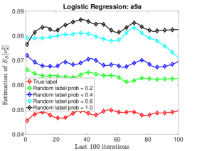
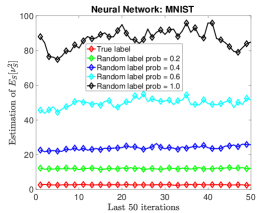
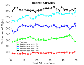
Figure 1: On-average variance of SGD v.s. random label probability.

Generalization Bound for SGD under Gradient Dominant Condition

In this section, we consider nonconvex loss functions with the empirical risk function $f_{S}$ further satisfying the following gradient dominance condition.

Definition 1.

Denote $f^{*}:=\inf_{\mathbf{w}\in\Omega}f(\mathbf{w})$. Then, the function $f$ is said to be $\gamma$-gradient dominant for $\gamma>0$ if

$$f(\mathbf{w})-f^{*}\leq\frac{1}{2\gamma}\|\nabla f(\mathbf{w})\|^{2},~{}\forall\mathbf{w}\in\Omega.$$ (5)

The gradient dominance condition (also referred to as Polyak-Łojasiewicz condition (?; ?)) guarantees a linear convergence of the function value sequence generated by gradient-based first-order methods (?). It is a condition that is much weaker than the strong convexity, and many nonconvex machine learning problems satisfy this condition around the global minimizers (?; ?).

The gradient dominance condition helps to improve the bound on the on-average stochastic gradient norm $\mathbb{E}_{\bm{\xi},S}\left[\|\nabla\ell(\mathbf{w}_{t,S};\mathbf{z}_{1})\|\right]$ (see Lemma 4 in the appendix), which is given by

$$\mathbb{E}_{\bm{\xi},S} \left[\|\nabla\ell(\mathbf{w}_{t,S};\mathbf{z}_{1})\|\right]$$

$$\leq\sqrt{2L\mathbb{E}_{S}[f_{S}^{*}]+\frac{1}{t}\bigg{(}2Lf(\mathbf{w}_{0})+\mathbb{E}_{S}[\nu_{S}^{2}]\bigg{)}}.$$ (6)

Compared to eq. 4 for general nonconvex functions, the above bound is further improved by a factor of $\frac{1}{t}$. This is because SGD converges sub-linearly to the optimum function value $f_{S}^{*}$ under the gradient dominance condition, and $\frac{1}{t}$ is essentially the convergence rate of SGD. In particular, for sufficiently large $t$, the on-average stochastic gradient norm is essentially bounded by $\sqrt{2L\mathbb{E}_{S}[f_{S}^{*}]}$, which is much smaller then the bound in eq. 4. With the bound in eq. 6, we obtain the following theorem.

Theorem 2.

(Mean Square Bound) Suppose $\ell$ is nonconvex, and $f_{S}$ is $\gamma$-gradient dominant ($\gamma<L$). Let Assumptions 1 and 2 hold. Apply the SGD to solve the ERM with the data set $S$ and choose $\alpha_{t}=\frac{c}{(t+2)\log(t+2)}$ with $0<c<\min\{\frac{1}{L},\frac{1}{2\gamma}\}$. Then, the following bound holds.

$$\mathbb{E}_{\bm{\xi},S}[|f_{S}(\mathbf{w}_{T,S})-f(\mathbf{w}_{T,S})|^{2}]\leq$$

$$\!\frac{2M^{2}}{n}\!+\!\frac{24M\sigma c}{n}\bigg{(}\!\!\!\sqrt{\!2L\mathbb{E}_{S}[f_{S}^{*}]}\log T\!+\!\sqrt{\!2Lf(\!\mathbf{w}_{0}\!)\!+\!2\mathbb{E}_{S}[\nu_{S}^{2}]}\!\bigg{)}.$$

The above bound for the mean square generalization error under gradient dominance condition improves that for general nonconvex functions in 1, as the dominant term (i.e., $\log T$-dependent term) has coefficient $\sqrt{2L\mathbb{E}_{S}[f_{S}^{*}]}$, which is much smaller than the term $\sqrt{2Lf(\mathbf{w}_{0})+\frac{1}{2}\mathbb{E}_{S}[\nu_{S}^{2}]}$ in the bound of 1. As an intuitively understanding, the on-average variance of the SGD is further reduced by its fast convergence rate $\frac{1}{t}$ under the gradient dominance condition. This results in a more stable on-average iterate stability which in turn improves the mean square generalization error. We note that (?) also studied the generalization error of SGD for loss functions satisfying both the gradient dominance condition and an additional quadratic growth condition. They also assumed that the algorithm converges to a global minimizer point, which may not always hold for noisy algorithms like SGD.

2 directly implies the following probabilistic guarantee for the generalization error of SGD.

Theorem 3.

(Bound with Probabilistic Guarantee) Suppose $\ell$ is nonconvex, and $f_{S}$ is $\gamma$-gradient dominant ($\gamma<L$). Let Assumptions 1 and 2 hold. Apply the SGD to solve the ERM with the data set $S$, and choose $\alpha_{t}=\frac{c}{(t+2)\log(t+2)}$ with $0<c<\min\{\frac{1}{L},\frac{1}{2\gamma}\}$. Then, for any $\delta>0$, with probability at least $1-\delta$, we have

$$|f_{S}(\mathbf{w}_{T,S})-f(\mathbf{w}_{T,S})|\leq$$

$$\!\!\sqrt{\!\tfrac{2M^{2}}{n\delta}\!+\!\tfrac{24M\sigma c}{n\delta}\bigg{(}\!\!\!\sqrt{\!2L\mathbb{E}_{S}[f_{S}^{*}]}\log T\!+\!\sqrt{\!2Lf(\!\mathbf{w}_{0}\!)\!+\!2\mathbb{E}_{S}[\nu_{S}^{2}]}\bigg{)}}.$$

Regularized Nonconvex Optimization

In practical applications, regularization is usually applied to the risk minimization problem in order to either promote certain structures on the desired solution or to restrict the parameter space. In this section, we explore how regularization can improve the generation error, and hence help to avoid overfitting for SGD.

Here, for any weight $\lambda>0$, we consider the regularized population risk minimization (R-PRM) and the regularized empirical risk minimization (R-ERM):

$$\min_{\mathbf{w}\in\Omega}~{}\Phi(\mathbf{w}):=f(\mathbf{w})+\lambda h(\mathbf{w}),$$

$$\min_{\mathbf{w}\in\Omega}~{}\Phi_{S}(\mathbf{w}):=f_{S}(\mathbf{w})+\lambda h(\mathbf{w}),$$

where $h$ corresponds to the regularizer and $f,f_{S}$ are the population and empirical risks, respectively. In particular, we are interested in the following class of regularizers.

Assumption 3.

The regularizer function $h$ is 1-strongly convex and nonnegative.

Without loss of generality, we assume that the strongly convex parameter of $h$ is 1, and this can be adjusted by scaling the weight parameter $\lambda$. Strongly convex regularizers are commonly used in machine learning applications, and typical examples include $\frac{\lambda}{2}\|\mathbf{w}\|^{2}$ for ridge regression, Tikhonov regularization $\frac{\lambda}{2}\|\Gamma\mathbf{w}\|^{2}$ and elastic net $\lambda_{1}\|\mathbf{w}\|_{1}\!+\!\lambda_{2}\|\mathbf{w}\|^{2}$, etc. Here, we allow the regularizer $h$ to be non-differentiable (e.g., the elastic net), and introduce the following proximal mapping with parameter $\alpha>0$ to deal with the non-smoothness.

$$\mathrm{prox}_{\alpha h}(\mathbf{w}):=\arg\min_{\mathbf{u}\in\Omega}h(\mathbf{u})+\frac{1}{2\alpha}\|\mathbf{u}-\mathbf{w}\|^{2}.$$ (7)

The proximal mapping is the core of the proximal method for solving convex problems (?; ?) and nonconvex ones (?; ?). In particular, we apply the proximal SGD to solve the R-ERM. With the same notations as those defined in the previous section, the update rule of the proximal SGD can be written as, for $t=0,\ldots,T-1$

$$\mathbf{w}_{t+1}=\mathrm{prox}_{\alpha_{t}h}\big{(}\mathbf{w}_{t}-\alpha_{t}\nabla\ell(\mathbf{w}_{t};\mathbf{z}_{\xi_{t}})\big{)}.$$ (proximal-SGD)

Similarly, we denote $\{\mathbf{w}_{t,S}\}_{t}$ as the iterate sequence generated by the proximal SGD with the data set $S$.

It is clear that the generalization error of the function value for the regularized risk minimization, i.e., $|\Phi(\mathbf{w}_{T,S})-\Phi_{S}(\mathbf{w}_{T,S})|$, is the same as that for the un-regularized risk minimization. Hence, Proposition 1 is also applicable to the mean square generalization error of the regularized risk minimization. However, the development of the generalization error bound is different from the analysis in the previous section from two aspects. First, the analysis of the on-average iterate stability of the proximal SGD is technically more involved than that of SGD due to the possibly non-smooth regularizer. Secondly, the proximal mappings of strongly convex functions are strictly contractive (see item 2 of Lemma 5 in the appendix). Thus, the proximal step in the proximal SGD enhances the stability between the iterates $\mathbf{w}_{t,S}$ and $\mathbf{w}_{t,\overline{S}}$ that are generated by the algorithm using perturbed datasets, and this further improves the generalization error. The next result provides a quantitative statement.

Theorem 4.

Consider the regularized risk minimization. Suppose $\ell$ is nonconvex. Let Assumptions 1, 2 and 3 hold, and apply the proximal SGD to solve the R-ERM with the dataset $S$. Let $\lambda>L$ and $\alpha_{t}=\frac{c}{t+2}$ with $0<c<\frac{1}{L}$. Then, the following bound holds with probability at least $1-\delta$.

$$|\Phi(\mathbf{w}_{T,S}) -\Phi_{S}(\mathbf{w}_{T,S})|$$

$$\leq\sqrt{\frac{1}{n\delta}\Big{(}2M^{2}+\frac{24M\sigma}{(\lambda-L)}\sqrt{L\Phi(\mathbf{w}_{0})+\mathbb{E}_{S}[\nu_{S}^{2}]}\Big{)}}.$$

4 provides probabilistic guarantee for the generalization error of the proximal SGD in terms of the on-average variance of the stochastic gradients. Comparison of 4 with 1 indicates that a strongly convex regularizer substantially improves the generalization error bound of SGD for nonconvex loss functions by removing the logarithm dependence on $T$. It is also interesting to compare 4 with [Proposition 4 and Theorem 1, (?)], which characterize the generalization error of SGD for strongly convex functions with probabilistic guarantee. The two bounds have the same order in terms of $n$ and $T$, indicating that a strongly convex regularizer even improves the generalization error for a nonconvex function to be the same as that for a strongly convex function. In practice, the regularization weight $\lambda$ should be properly chosen to balance between the generalization error and the training loss, as otherwise the parameter space can be too restrictive to yield a good solution for the risk function.

We further conduct experiments to explore the effect of regularization on the generalization error by adding the regularizer $\frac{\lambda}{2}\|\mathbf{w}\|^{2}$ to the objective functions. In particular, we apply the proximal SGD to solve the logistic regression (with dataset a9a) and train the neural network (with dataset MNIST) mentioned in the previous section. Figure 2 shows the results where the left axis denotes the scale of the training error and the right axis denotes the scale of the generalization error. It can be seen that the corresponding generalization errors improve as the regularization weight gets large. This agrees with our theoretical finding on the impact of regularization. On the other hand, the training performances for both problems degrade as the regularization weight increases, which is reasonable because in such a case the optimization focuses too much on the regularizer and the obtained solution does not minimize the loss function well. Hence, there is a trade-off between the training and generalization performance in tuning the regularization parameter.

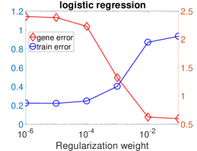
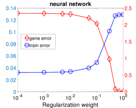
Figure 2: Generalization error v.s. regularization parameter.

Generalization Bound with High-Probability Guarantee

The studies of the previous sections explore the probabilistic guarantee for the generalization errors of nonconvex loss functions and nonconvex loss functions with strongly convex regularizers. For example, apply SGD to solve a generic nonconvex loss function, then 1 suggests that for any $\epsilon>0$,

$$\mathbb{P}(|f(\mathbf{w}_{T,S})-f_{S}(\mathbf{w}_{T,S})|>\epsilon)<O\Big{(}\frac{\log T}{n\epsilon^{2}}\Big{)},$$

which decays sublinearly as $\frac{n}{\log T}\to\infty$. In this subsection, we study a stronger probabilistic guarantee for the generalization error, i.e., the probability for it to be less than $\epsilon$ decays exponentially. We refer to such a notion as high-probability guarantee. In particular, we explore for which cases of nonconvex loss functions we can establish such a stronger performance guarantee.

Towards this end, we adopt the uniform stability framework proposed in (?). Note that (?) also studied the uniform stability of SGD, but only characterized the generalization error in expectation, which is weaker than the exponential probabilistic concentrtion bound that we study here.

Suppose we apply SGD with the same sample path $\bm{\xi}$ to solve the ERM with the datasets $S$ and $\overline{S}$, respectively, and denote $\mathbf{w}_{T,S,\bm{\xi}}$ and $\mathbf{w}_{T,\overline{S},\bm{\xi}}$ as the corresponding outputs. Also, suppose we apply the SGD with different sample paths $\bm{\xi}$ and $\overline{\bm{\xi}}$ to solve the same problem with the dataset $S$, respectively, and denote $\mathbf{w}_{T,S,\bm{\xi}}$ and $\mathbf{w}_{T,S,\overline{\bm{\xi}}}$ as the corresponding outputs. Here, $\overline{\bm{\xi}}$ denotes the sample path that replaces one of the sampled indices, say $\xi_{t_{0}}$, with an i.i.d copy $\xi_{t_{0}}^{\prime}$. The following result is a variant of [Theorem 15, (?)].

Lemma 1.

Let 1 hold. If SGD satisfies the following conditions

$$\sup_{S,\overline{S},\mathbf{z}}\mathbb{E}_{\bm{\xi}}|\ell(\mathbf{w}_{T,S,\bm{\xi}};\mathbf{z})-\ell(\mathbf{w}_{T,\overline{S},\bm{\xi}};\mathbf{z})|\leq\beta,$$

$$\sup_{\bm{\xi},\overline{\bm{\xi}},S,\mathbf{z}}|\ell(\mathbf{w}_{T,S,\bm{\xi}};\mathbf{z})-\ell(\mathbf{w}_{T,S,\overline{\bm{\xi}}};\mathbf{z})|\leq\rho.$$

Then, the following bound holds with probability at least $1-\delta$.

$$|\Phi(\mathbf{w}_{T,S})- \Phi_{S}(\mathbf{w}_{T,S})|$$

$$\leq 2\beta+\left(\frac{M+4n\beta}{\sqrt{2n}}+\sqrt{2T}\rho\right)\sqrt{\log\tfrac{2}{\delta}}.$$

Note that Lemma 1 implies that

$$\mathbb{P}(|\Phi(\mathbf{w}_{T,S})-\Phi_{S}(\mathbf{w}_{T,S})|>\epsilon)\leq O\bigg{(}\exp\Big{(}\tfrac{-\epsilon^{2}}{\sqrt{n}\beta+\sqrt{T}\rho}\Big{)}\bigg{)}.$$

Hence, if $\beta=o(n^{-\frac{1}{2}})$ and $\rho=o(T^{-\frac{1}{2}})$, then we have exponential decay in probability as $n\rightarrow\infty$ and $T\rightarrow\infty$. It turns out that our analysis of the uniform stability of SGD for general nonconvex functions yields that $\beta=O(n^{-1}),\rho=O(\log T)$, which does not lead to the desired high-probability guarantee for the generalization error. On the other hand, the analysis of the uniform stability of the proximal SGD for nonconvex loss functions with strongly convex regularizers yields that $\beta=O(n^{-1}),\rho=O(T^{-c(\lambda-L)}),$ which leads to the high-probability guarantee if we choose $\lambda>L$ and $c>\frac{1}{2(\lambda-L)}$. This further demonstrates that a strongly convex regularizer can significantly improve the quality of the probabilistic bound for the generalization error. The following result is a formal statement of the above discussion.

Theorem 5.

Consider the regularized risk minimization with the nonconvex loss function $\ell$. Let Assumptions 1 and 3 hold, and apply the proximal SGD to solve the R-ERM with the data set $S$. Choose $\lambda>L$ and $\alpha_{t}=\frac{c}{t+2}$ with $\frac{1}{2(\lambda-L)}<c<\frac{1}{\lambda-L}$. Then, the following bound holds with probability at least $1-\delta$

$$|\Phi(\mathbf{w}_{T,S}) -\Phi_{S}(\mathbf{w}_{T,S})|$$

$$\leq\Big{(}\frac{M}{\sqrt{n}}+\frac{4\sigma^{2}}{\sqrt{n}(\lambda-L)}+\frac{4\sigma^{2}c}{T^{c(\lambda-L)-\frac{1}{2}}}\Big{)}\sqrt{\log\frac{2}{\delta}}.$$

5 implies that

$$\mathbb{P}(|\Phi(\mathbf{w}_{T,S}) -\Phi_{S}(\mathbf{w}_{T,S})|>\epsilon)$$

$$\leq O\bigg{(}\exp\Big{(}\tfrac{-\epsilon^{2}}{n^{-\frac{1}{2}}+T^{\frac{1}{2}-c(\lambda-L)}}\Big{)}\bigg{)}.$$

Hence, if we choose $c=\frac{1}{\lambda-L}$ and run the proximal SGD for $T=O(n)$ iterations (i.e., constant passes over the data), then the probability of the event decays exponentially as $O(\exp(-\sqrt{n}\epsilon^{2}))$.

The proof of 5 characterizes the uniform iterate stability of the proximal SGD with regard to the perturbations of both the dataset and the sample path. Unlike the on-average stability in 1 where the stochastic gradient norm is bounded by the on-average variance of the stochastic gradients, the uniform stability captures the worst case among all datasets, and hence uses the uniform upper bound $\sigma$ for the stochastic gradient norm.

We note that [Theorem 3, (?)] also established a probabilistic bound under the PAC Bayesian framework. However, their result yields exponential concentration guarantee only for strongly convex loss functions. As a comparison, 5 relaxes the requirement of strong convexity for loss functions to nonconvex loss functions with strongly convex regularizers, and hence serves as a complementary result to theirs. Also, (?) establishes the high-probability bound for the generalization error of SGD with regularization. However, their result holds only for the particular regularizer $\frac{1}{2}\|\mathbf{w}\|^{2}$, and high-probability bound holds only with regard to the random draw of the data. As a comparison, our result holds for all strongly convex regularizers, and the high-probability bound hold with regard to both the draw of data and randomness of algorithm.

Conclusion

In this paper, we develop the generalization error bound of SGD with probabilistic guarantee for nonconvex optimization. We obtain the improved bounds based on the variance of the stochastic gradients by exploiting the optimization path of SGD. Our generalization bound is consistent with the effect of random labels on the generalization error that observed in practical experiments. We further show that strongly convex regularizers can significantly improve the probabilistic concentration bounds for the generalization error from the sub-linear rate to the exponential rate. Our study demonstrates that the geometric structure of the problem can be an important factor in improving the generalization performance of algorithms. Thus, it is of interest to explore the generalization error under various geometric conditions of the objective function in the future work.

Appendix A Proof of Main Results

Proof of Proposition 1

The proof is based on [Lemma 11, (?)] and 1. Denote $S^{i}$ as the data set that replaces the $i$-th sample of $S$ with an i.i.d. copy generated from the distribution $\mathcal{D}$. Following from Lemma 11 of (?), we obtain

$$\mathbb{E}_{S,\bm{\xi}}|f_{S}(\mathbf{w}_{T,S})-f(\mathbf{w}_{T,S})|^{2} \leq\frac{2M^{2}}{n}+\frac{12M}{n}\sum_{i=1}^{n}\mathbb{E}_{\bm{\xi},S,S^{i}}\left[|\ell(\mathbf{w}_{T,S};\mathbf{z}_{i})-\ell(\mathbf{w}_{T,S^{i}};\mathbf{z}_{i})|\right]$$

$$\leq\frac{2M^{2}}{n}+\frac{12M\sigma}{n}\sum_{i=1}^{n}\mathbb{E}_{\bm{\xi},S,S^{i}}\|\mathbf{w}_{T,S}-\mathbf{w}_{T,S^{i}}\|$$

$$=\frac{2M^{2}}{n}+12M\sigma\mathbb{E}_{\bm{\xi},S,\overline{S}}\|\mathbf{w}_{T,S}-\mathbf{w}_{T,\overline{S}}\|,$$

where the second inequality uses the Lipschitz property of the loss function in 1, and the last equality is due to the fact that the perturbed samples in $S^{i}$ and $\overline{S}$ are generated i.i.d from the underlying distribution.

Proof of 1

The proof is based on the following two important lemmas, which we prove first.

Lemma 2.

Let 1 hold. Apply SGD with the same sample path $\bm{\xi}$ to solve the ERM with data sets $S$ and $\overline{S}$, respectively. Choose $\alpha_{t}=\frac{c}{(t+2)\log(t+2)}$ with $0<c<\frac{1}{L}$, then the following bound holds.

$$\mathbb{E}_{S,\overline{S},\bm{\xi}}[\delta_{t+1,S,\overline{S}}] \leq(1+\alpha_{t}L)\mathbb{E}_{S,\overline{S},\bm{\xi}}[\delta_{t,S,\overline{S}}]+\frac{2\alpha_{t}}{n}\mathbb{E}_{S,\bm{\xi}}\left[\left\|\nabla\ell(\mathbf{w}_{t,S};\mathbf{z}_{1})\right\|\right].$$

Proof of Lemma 2.

Consider the two fixed data sets $S$ and $\overline{S}$ that differ at, say, the first data sample. At the $t$-th iteration, we consider two cases of the sampled index ${\xi_{t}}$. In the first case, $1\notin{\xi_{t}}$ (w.p. $\frac{n-1}{n}$), i.e., the sampled data from $S$ and $\overline{S}$ are the same, and we obtain that

$$\delta_{t+1,S,\overline{S}} =\left\|\mathbf{w}_{t,S}-\alpha_{t}\nabla\ell(\mathbf{w}_{t,S};\mathbf{z}_{\xi_{t}})-\mathbf{w}_{t,\overline{S}}+\alpha_{t}\nabla\ell(\mathbf{w}_{t,\overline{S}};\mathbf{z}_{\xi_{t}})\right\|$$

$$\leq\delta_{t,S,\overline{S}}+\alpha_{t}\left\|\nabla\ell(\mathbf{w}_{t,S};\mathbf{z}_{\xi_{t}})-\nabla\ell(\mathbf{w}_{t,\overline{S}};\mathbf{z}_{\xi_{t}})\right\|$$

$$\leq(1+\alpha_{t}L)\delta_{t,S,\overline{S}},$$ (8)

where the last inequality uses the $L$-Lipschitz property of $\nabla\ell$. In the other case, $1\in{\xi_{t}}$ (w.p. $\frac{1}{n}$), we obtain that

$$\delta_{t+1,S,\overline{S}} =\left\|\mathbf{w}_{t,S}-\alpha_{t}\nabla\ell(\mathbf{w}_{t,S};\mathbf{z}_{1})-\mathbf{w}_{t,\overline{S}}+\alpha_{t}\nabla\ell(\mathbf{w}_{t,\overline{S}};\mathbf{z}_{1}^{\prime})\right\|$$

$$\leq\delta_{t,S,\overline{S}}+\alpha_{t}\left\|\nabla\ell(\mathbf{w}_{t,S};\mathbf{z}_{1})-\nabla\ell(\mathbf{w}_{t,\overline{S}};\mathbf{z}_{1}^{\prime})\right\|$$

$$\leq\delta_{t,S,\overline{S}}+\alpha_{t}\left(\left\|\nabla\ell(\mathbf{w}_{t,S};\mathbf{z}_{1})\right\|+\|\nabla\ell(\mathbf{w}_{t,\overline{S}};\mathbf{z}_{1}^{\prime})\|\right).$$ (9)

Combining the above two cases and taking expectation with respect to all randomness, we obtain that

$$\mathbb{E}_{S,\overline{S},\bm{\xi}}[\delta_{t+1,S,\overline{S}}] \leq\left[\frac{n-1}{n}(1+\alpha_{t}L)+\frac{1}{n}\right]\mathbb{E}_{S,\overline{S},\bm{\xi}}[\delta_{t,S,\overline{S}}]+\frac{1}{n}\alpha_{t}\mathbb{E}_{S,\overline{S},\bm{\xi}}\left(\left\|\nabla\ell(\mathbf{w}_{t,S};\mathbf{z}_{1})\right\|+\|\nabla\ell(\mathbf{w}_{t,\overline{S}};\mathbf{z}_{1}^{\prime})\|\right)$$

$$\overset{(i)}{\leq}(1+\alpha_{t}L)\mathbb{E}_{S,\overline{S},\bm{\xi}}[\delta_{t,S,\overline{S}}]+\frac{2\alpha_{t}}{n}\mathbb{E}_{S,\bm{\xi}}\left[\left\|\nabla\ell(\mathbf{w}_{t,S};\mathbf{z}_{1})\right\|\right],$$ (10)

where (i) uses the fact that $\mathbf{z}_{1}^{\prime}$ is an i.i.d. copy of $\mathbf{z}_{1}$. ∎

Lemma 3.

Let Assumptions 1 and 2 hold. Apply SGD to solve the ERM with data set $S$ and choosing $\alpha_{t}\leq\frac{c}{t+2}$ for some $0<c<\frac{1}{L}$. Then, the following bound holds.

$$\mathbb{E}_{\bm{\xi},S}\left[\|\nabla\ell(\mathbf{w}_{t,S};\mathbf{z}_{1})\|\right]\leq\sqrt{2Lf(\mathbf{w}_{0})+\frac{1}{2}\mathbb{E}_{S}[\nu_{S}^{2}]}.$$

Proof of Lemma 3.

By 1, $\ell$ is nonnegative and $\nabla\ell$ is $L$-Lipschitz. Then, eq. (12.6) of (?) shows that

$$\forall\mathbf{w},\quad\|\nabla\ell(\mathbf{w};\mathbf{z})\|\leq\sqrt{2L\ell(\mathbf{w};\mathbf{z})}.$$ (11)

Based on eq. 11, we further obtain that

$$\mathbb{E}_{\bm{\xi},S}\|\nabla\ell(\mathbf{w}_{t,S};\mathbf{z}_{1})\| \leq\sqrt{2L}\mathbb{E}_{\bm{\xi},S}\sqrt{\ell(\mathbf{w}_{t,S};\mathbf{z}_{1})}\overset{(i)}{\leq}\sqrt{2L}\sqrt{\mathbb{E}_{\bm{\xi},S}\ell(\mathbf{w}_{t,S};\mathbf{z}_{1})}$$

$$\overset{(ii)}{\leq}\sqrt{2L}\sqrt{\mathbb{E}_{\bm{\xi},S}\frac{1}{n}\sum_{j=1}^{n}\ell(\mathbf{w}_{t,S};\mathbf{z}_{j})}=\sqrt{2L}\sqrt{\mathbb{E}_{\bm{\xi},S}f_{S}(\mathbf{w}_{t,S})},$$ (12)

where (i) uses the Jesen’s inequality and (ii) uses the fact that all samples in $S$ are generated i.i.d. from $\mathcal{D}$.

Next, consider a fixed data set $S$ and denote $\mathbf{g}_{t,S}=\nabla\ell(\mathbf{w}_{t,S};\mathbf{z}_{\xi_{t}})$ as the sampled stochastic gradient at iteration $t$. Then, by smoothness of $\ell$ and the update rule of the SGD, we obtain that

$$f_{S}(\mathbf{w}_{t+1,S})-f_{S}(\mathbf{w}_{t,S}) \leq\langle\mathbf{w}_{t+1,S}-\mathbf{w}_{t,S},\nabla f_{S}(\mathbf{w}_{t,S})\rangle+\frac{L}{2}\|\mathbf{w}_{t+1,S}-\mathbf{w}_{t,S}\|^{2}$$

$$=\langle-\alpha_{t}\mathbf{g}_{t,S},\nabla f_{S}(\mathbf{w}_{t,S})\rangle+\frac{L\alpha_{t}^{2}}{2}\left\|\mathbf{g}_{t,S}\right\|^{2}.$$

Conditioning on $\mathbf{w}_{t,S}$ and taking expectation with respect to $\bm{\xi}$, we further obtain from the above inequality that

$$\mathbb{E}_{\bm{\xi}} \left[f_{S}(\mathbf{w}_{t+1,S})-f_{S}(\mathbf{w}_{t,S})|\mathbf{w}_{t,S}\right]$$

$$\leq\left(\frac{L\alpha_{t}^{2}}{2}-\alpha_{t}\right)\left\|\nabla f_{S}(\mathbf{w}_{t,S})\right\|^{2}+\frac{L\alpha_{t}^{2}}{2}\mathbb{E}_{\bm{\xi}}\left[\left\|\mathbf{g}_{t,S}\right\|^{2}-\left\|\nabla f_{S}(\mathbf{w}_{t,S})\right\|^{2}|\mathbf{w}_{t,S}\right].$$ (13)

Note that $\frac{L\alpha_{t}^{2}}{2}-\alpha_{t}<0$ by our choice of stepsize. Further taking expectation with respect to the randomness of $\mathbf{w}_{t,S}$ and $S$, and telescoping the above inequality over $0,\ldots,t-1$, we obtain that

$$\mathbb{E}_{\bm{\xi},S}\left[f_{S}(\mathbf{w}_{t,S})\right] \overset{(i)}{\leq}\mathbb{E}_{S}f_{S}(\mathbf{w}_{0})+\sum_{t^{\prime}=0}^{t-1}\frac{L\alpha_{t^{\prime}}^{2}}{2}\mathbb{E}_{S}[\nu_{S}^{2}]$$

$$=f(\mathbf{w}_{0})+\sum_{t^{\prime}=0}^{t-1}\frac{Lc^{2}\mathbb{E}_{S}[\nu_{S}^{2}]}{2(t^{\prime}+2)^{2}}\overset{(ii)}{\leq}f(\mathbf{w}_{0})+\frac{Lc^{2}\mathbb{E}_{S}[\nu_{S}^{2}]}{4},$$

where (i) uses the fact that the variance of the stochastic gradients is bounded by $\mathbb{E}_{S}[\nu_{S}^{2}]$, and (ii) upper bounds the summation by the integral, i.e., $\sum_{t^{\prime}=0}^{t-1}\frac{1}{(t^{\prime}+2)^{2}}\lesssim\int_{1}^{t}\frac{1}{t^{\prime 2}}dt^{\prime}$. Substituting the above result into eq. 12 and noting that $cL\leq 1$, we obtain the desired result. ∎

Now by Lemma 2, we obtain that

$$\mathbb{E}_{S,\overline{S},\bm{\xi}}[\delta_{t+1,S,\overline{S}}] \leq(1+\alpha_{t}L)\mathbb{E}_{S,\overline{S},\bm{\xi}}[\delta_{t,S,\overline{S}}]+\frac{2\alpha_{t}}{n}\mathbb{E}_{S,\bm{\xi}}\left[\left\|\nabla\ell(\mathbf{w}_{t,S};\mathbf{z}_{1})\right\|\right]$$

$$\overset{(i)}{\leq}(1+\alpha_{t}L)\mathbb{E}_{S,\overline{S},\bm{\xi}}[\delta_{t,S,\overline{S}}]+\frac{2\alpha_{t}\sqrt{2Lf(\mathbf{w}_{0})+\frac{\mathbb{E}_{S}[\nu_{S}^{2}]}{2}}}{n},$$ (14)

where (i) applies Lemma 3. Recursively applying eq. 14 over $t=0,\ldots,T-1$ and noting that $\delta_{0}=0$ and $\alpha_{t}=\frac{c}{(t+2)\log(t+2)}$, we obtain

$$\mathbb{E}_{S,\overline{S},\bm{\xi}}[\delta_{T}] \leq\sum_{t=0}^{T-1}\left[\prod_{k=t+1}^{T-1}(1+\alpha_{k}L)\right]\frac{2c\sqrt{2Lf(\mathbf{w}_{0})+\frac{\mathbb{E}_{S}[\nu_{S}^{2}]}{2}}}{(t+2){\log(t+2)}n}$$

$$\overset{(i)}{\leq}\sum_{t=0}^{T-1}\left[\exp\left(\sum_{k=t+1}^{T-1}\frac{cL}{(k+2)\log(k+2)}\right)\right]\frac{2c\sqrt{2Lf(\mathbf{w}_{0})+\frac{\mathbb{E}_{S}[\nu_{S}^{2}]}{2}}}{(t+2){\log(t+2)}n}$$

$$\overset{(ii)}{\leq}\sum_{t=0}^{T-1}\left(\frac{\log T}{\log(t+2)}\right)^{cL}\frac{2c\sqrt{2Lf(\mathbf{w}_{0})+\frac{\mathbb{E}_{S}[\nu_{S}^{2}]}{2}}}{(t+2){\log(t+2)}n}$$

$$\overset{(iii)}{\leq}\frac{2c\sqrt{2Lf(\mathbf{w}_{0})+\frac{\mathbb{E}_{S}[\nu_{S}^{2}]}{2}}}{n}\log T,$$

where (i) uses the fact that $1+x\leq\exp(x)$. For (ii) and (iii), we apply the integral upper bounds to bound the summations, i.e., $\sum_{k=t+1}^{T-1}\frac{cL}{(k+2)\log(k+2)}\lesssim\int_{t}^{T}\frac{cL}{k\log k}dk,\sum_{t=0}^{T-1}(t+2)^{-1}\log^{-1-cL}(t+2)\lesssim\int_{t=1}^{T}t^{-1}\log^{-1-cL}tdt$, and use the fact that $cL<1$. Substituting the above result into Proposition 1 and applying the Chebyshev’s inequality yields the desired result.

Proof of 2

We first prove a useful lemma.

Lemma 4.

Let Assumptions 1 and 2 hold. Apply the SGD to solve the ERM with data set $S$, where $f_{S}$ is $\gamma$-gradient dominant ($\gamma<L$) with the minimum function value $f_{S}^{*}$. Suppose we choose $\alpha_{t}\leq\frac{c}{t+2}$ for some $0<c<\min\{\frac{2}{\gamma},\frac{1}{L}\}$. Then the following bound holds.

$$\mathbb{E}_{\bm{\xi},S}\left[\|\nabla\ell(\mathbf{w}_{t,S};\mathbf{z}_{1})\|\right]\leq\sqrt{2L\mathbb{E}_{S}[f_{S}^{*}]+\frac{1}{t}\left(2Lf(\mathbf{w}_{0})+2\mathbb{E}_{S}[\nu_{S}^{2}]\right)}.$$

Proof of Lemma 4.

We first note that eq. 12 and eq. 13 both hold here, which we rewritten below for convenience.

$$\mathbb{E}_{\bm{\xi},S}\|\nabla\ell(\mathbf{w}_{t,S};\mathbf{z}_{1})\| \leq\sqrt{2L}\sqrt{\mathbb{E}_{\bm{\xi},S}f_{S}(\mathbf{w}_{t,S})},$$ (15)

$$\mathbb{E}_{\bm{\xi}} \left[f_{S}(\mathbf{w}_{t+1,S})-f_{S}(\mathbf{w}_{t,S})|\mathbf{w}_{t,S}\right]$$

$$\leq\left(\frac{L\alpha_{t}^{2}}{2}-\alpha_{t}\right)\left\|\nabla f_{S}(\mathbf{w}_{t,S})\right\|^{2}+\frac{L\alpha_{t}^{2}}{2}\mathbb{E}_{\bm{\xi}}\left[\left\|\mathbf{g}_{t,S}\right\|^{2}-\left\|\nabla f_{S}(\mathbf{w}_{t,S})\right\|^{2}|\mathbf{w}_{t,S}\right].$$ (16)

Following from eq. 16 and the fact that $f_{S}$ is $\gamma$-gradient dominant, we obtain

$$\mathbb{E}_{\bm{\xi}}\left[f_{S}(\mathbf{w}_{t+1,S})-f_{S}(\mathbf{w}_{t,S})~{}|~{}\mathbf{w}_{t,S}\right]$$

$$\leq\left(\frac{L\alpha_{t}^{2}}{2}-\alpha_{t}\right)2\gamma(f_{S}(\mathbf{w}_{t,S})-f_{S}^{*})+\frac{L\alpha_{t}^{2}}{2}\mathbb{E}_{\bm{\xi}}\left[\left\|g_{t,S}\right\|^{2}-\left\|\nabla f_{S}(\mathbf{w}_{t,S})\right\|^{2}~{}|~{}\mathbf{w}_{t,S}\right].$$ (17)

Further taking expectation with respect to the randomness of $\mathbf{w}_{t,S}$ and $S$, we obtain from the above inequality that

$$\mathbb{E}_{\bm{\xi},S}\left[f_{S}(\mathbf{w}_{t+1,S})-f_{S}(\mathbf{w}_{t,S})\right] \leq\left(\frac{L\alpha_{t}^{2}}{2}-\alpha_{t}\right)2\gamma\mathbb{E}_{\bm{\xi},S}(f_{S}(\mathbf{w}_{t,S})-f_{S}^{*})+\frac{L\alpha_{t}^{2}}{2}\mathbb{E}_{S}[\nu_{S}^{2}]$$

$$\leq-\alpha_{t}\gamma\mathbb{E}_{\bm{\xi},S}(f_{S}(\mathbf{w}_{t,S})-f_{S}^{*})+\frac{L\alpha_{t}^{2}\mathbb{E}_{S}[\nu_{S}^{2}]}{2},$$

where the last inequality uses the fact that $\frac{L\alpha_{t}^{2}}{2}\leq\alpha_{t}/2$ for $c<\frac{1}{L}$. Rearranging the above inequality, we further obtain that

$$\mathbb{E}_{\bm{\xi},S}\left[f_{S}(\mathbf{w}_{t+1,S})-f_{S}^{*}\right] \leq(1-\alpha_{t}\gamma)\mathbb{E}_{\bm{\xi},S}(f_{S}(\mathbf{w}_{t,S})-f_{S}^{*})+\frac{L\alpha_{t}^{2}\nu^{2}}{2}$$

$$\leq\prod_{t^{\prime}=0}^{t}(1-\alpha_{t^{\prime}}\gamma)\mathbb{E}_{S}(f_{S}(\mathbf{w}_{0})-f_{S}^{*})+\sum_{t^{\prime}=0}^{t}\prod_{k=t^{\prime}+1}^{t-1}(1-\alpha_{k}\gamma)\frac{L\alpha_{t^{\prime}}^{2}\mathbb{E}_{S}[\nu_{S}^{2}]}{2}$$

$$\overset{(i)}{\leq}t^{-c\gamma}\mathbb{E}_{S}(f_{S}(\mathbf{w}_{0})-f_{S}^{*})+\frac{Lc^{2}\mathbb{E}_{S}[\nu_{S}^{2}]}{t^{c\gamma}}$$

$$\overset{(ii)}{\leq}\frac{1}{t^{c\gamma}}\left[f(\mathbf{w}_{0})+Lc^{2}\mathbb{E}_{S}[\nu_{S}^{2}]\right],$$

where (i) uses the fact that $1-x\leq\exp(-x)$ and upper bounds the summations by the corresponding integrals, i.e., $\exp(-c\gamma\sum_{t^{\prime}=0}^{t}\frac{1}{t^{\prime}+2})\lesssim\exp(-c\gamma\int_{0}^{t}\frac{1}{t^{\prime}}dt^{\prime})$ and (ii) uses the fact that $c\gamma<1/2$. We then conclude that

$$\mathbb{E}_{\bm{\xi},S}f_{S}(\mathbf{w}_{t,S})\leq\mathbb{E}_{S}[f_{S}^{*}]+\frac{1}{t^{c\gamma}}\left[f(\mathbf{w}_{0})+L\nu^{2}c^{2}\right].$$

Substituting this bound into eq. 15 and noting that $cL\leq 1$, we obtain the desired result. ∎

To continue our proof, by Lemma 2, we obtain that

$$\mathbb{E}_{S,\overline{S},\bm{\xi}}[\delta_{t+1,S,\overline{S}}] \leq(1+\alpha_{t}L)\mathbb{E}_{S,\overline{S},\bm{\xi}}[\delta_{t,S,\overline{S}}]+\frac{2\alpha_{t}}{n}\mathbb{E}_{S,\bm{\xi}}\left[\left\|\nabla\ell(\mathbf{w}_{t,S};\mathbf{z}_{1})\right\|\right]$$

$$\leq(1+\alpha_{t}L)\mathbb{E}_{S,\overline{S},\bm{\xi}}[\delta_{t,S,\overline{S}}]+\frac{2\alpha_{t}}{n}\sqrt{2L\mathbb{E}_{S}[f_{S}^{*}]+\frac{1}{t^{c\gamma}}\left(2Lf(\mathbf{w}_{0})+2\mathbb{E}_{S}[\nu_{S}^{2}]\right)},$$ (18)

where the last line applies Lemma 4. Applying eq. 18 recursively over $t=0,\ldots,T-1$ and noting that $\delta_{0}=0,\alpha_{t}=\frac{c}{(t+2)\log(t+2)}$, we obtain that

$$\mathbb{E}_{S,\overline{S},\bm{\xi}}[\delta_{T}] \leq\sum_{t=0}^{T-1}\left[\prod_{k=t+1}^{T-1}(1+\alpha_{k}L)\right]\frac{2c}{(t+2)\log(t+2)n}\sqrt{2L\mathbb{E}_{S}[f_{S}^{*}]+\frac{1}{t^{c\gamma}}\left(2Lf(\mathbf{w}_{0})+2\mathbb{E}_{S}[\nu_{S}^{2}]\right)}$$

$$\leq\frac{2c}{n}\sum_{t=0}^{T-1}\left(\frac{\log T}{\log(t+2)}\right)^{cL}\frac{\sqrt{2L\mathbb{E}_{S}[f_{S}^{*}]}+\sqrt{\frac{1}{t^{c\gamma}}\left(2Lf(\mathbf{w}_{0})+2\mathbb{E}_{S}[\nu_{S}^{2}]\right)}}{(t+2)\log(t+2)}$$

$$\leq\frac{2c}{n}\left(\sqrt{2L\mathbb{E}_{S}[f_{S}^{*}]}\log T+\sqrt{2Lf(\mathbf{w}_{0})+2\mathbb{E}_{S}[\nu_{S}^{2}]}\right).$$

Substituting the above result into Proposition 1 yields the desired result.

Proof of 4

Consider the fixed data sets $S$ and $\overline{S}$ that are differ at the first sample. At the $t$-th iteration, if $1\notin{\xi_{t}}$ (w.p. $\frac{n-1}{n}$), we obtain that

$$\delta_{t+1,S,\overline{S}} =\left\|\mathrm{prox}_{\alpha_{t}h}\left(\mathbf{w}_{t,S}-\alpha_{t}\nabla\ell(\mathbf{w}_{t,S};\mathbf{z}_{\xi_{t}})\right)-\mathrm{prox}_{\alpha_{t}h}\left(\mathbf{w}_{t,\overline{S}}-\alpha_{t}\nabla\ell(\mathbf{w}_{t,\overline{S}};\mathbf{z}_{\xi_{t}})\right)\right\|$$

$$\overset{(i)}{\leq}\frac{1}{1+\alpha_{t}\lambda}\left\|\mathbf{w}_{t,S}-\alpha_{t}\nabla\ell(\mathbf{w}_{t,S};\mathbf{z}_{\xi_{t}})-\mathbf{w}_{t,\overline{S}}+\alpha_{t}\nabla\ell(\mathbf{w}_{t,\overline{S}};\mathbf{z}_{\xi_{t}})\right\|$$

$$\leq\frac{1+\alpha_{t}L}{1+\alpha_{t}\lambda}\delta_{t,S,\overline{S}},$$ (19)

where (i) uses item 2 of Lemma 5. On the other hand, if $1\in{\xi_{t}}$ (w.p. $\frac{1}{n}$), we obtain that

$$\delta_{t+1,S,\overline{S}} =\bigg{\|}\mathrm{prox}_{\alpha_{t}h}\left(\mathbf{w}_{t,S}-\alpha_{t}\nabla\ell(\mathbf{w}_{t,S};\mathbf{z}_{1})\right)-\mathrm{prox}_{\alpha_{t}h}\left(\mathbf{w}_{t,\overline{S}}-\alpha_{t}\nabla\ell(\mathbf{w}_{t,\overline{S}};\mathbf{z}_{1}^{\prime})\right)\bigg{\|}$$

$$\overset{(i)}{\leq}\frac{1}{1+\alpha_{t}\lambda}\left\|\mathbf{w}_{t,S}-\alpha_{t}\nabla\ell(\mathbf{w}_{t,S};\mathbf{z}_{1})-\mathbf{w}_{t,\overline{S}}+\alpha_{t}\nabla\ell(\mathbf{w}_{t,\overline{S}};\mathbf{z}_{1}^{\prime})\right\|$$

$$\leq\frac{1}{1+\alpha_{t}\lambda}\delta_{t,S,\overline{S}}+\frac{\alpha_{t}}{1+\alpha_{t}\lambda}\left(\|\nabla\ell(\mathbf{w}_{t,S};\mathbf{z}_{1})\|+\|\nabla\ell(\mathbf{w}_{t,\overline{S}};\mathbf{z}_{1}^{\prime})\|\right),$$ (20)

where (i) uses item 2 of Lemma 5. Combining the above two cases and taking expectation with respect to the randomness of $\bm{\xi}$, $S$ and $\overline{S}$, we obtain that

$$\mathbb{E}_{S,\overline{S},\bm{\xi}}[\delta_{t+1,S,\overline{S}}] \leq\left[\frac{n-1}{n}\frac{1+\alpha_{t}L}{1+\alpha_{t}\lambda}+\frac{1}{n}\frac{1}{1+\alpha_{t}\lambda}\right]\mathbb{E}_{S,\overline{S},\bm{\xi}}[\delta_{t,S,\overline{S}}]+\frac{1}{n}\frac{2\alpha_{t}}{1+\alpha_{t}\lambda}\mathbb{E}_{S,\bm{\xi}}\|\nabla\ell(\mathbf{w}_{t,S};\mathbf{z}_{1})\|$$

$$\overset{(i)}{\leq}\frac{1+\alpha_{t}L}{1+\alpha_{t}\lambda}\mathbb{E}_{S,\overline{S},\bm{\xi}}[\delta_{S,\overline{S},\bm{\xi}}]+\frac{2\alpha_{t}}{n}\frac{1}{1+\alpha_{t}\lambda}\sqrt{2L\Phi(\mathbf{w}_{0})+2\mathbb{E}_{S}[\nu_{S}^{2}]\log t}$$

$$\lesssim\exp(\alpha_{t}(L-\lambda))\mathbb{E}_{S,\overline{S},\bm{\xi}}[\delta_{S,\overline{S},\bm{\xi}}]+\frac{2\alpha_{t}}{n}\sqrt{2L\Phi(\mathbf{w}_{0})+2\mathbb{E}_{S}[\nu_{S}^{2}]\log t},$$

where (i) uses Lemma 6. Recursively applying the above inequality over $t=0,\ldots,T-1$ and noting that $\delta_{0}=0,\alpha_{t}=\frac{c}{t+2}$, we obtain that

$$\mathbb{E}_{S,\overline{S},\bm{\xi}}[\delta_{T,S,\overline{S}}] \leq\sum_{t=0}^{T-1}\left[\prod_{k=t+1}^{T-1}\exp(\alpha_{k}(L-\lambda))\right]\frac{2c\sqrt{2L\Phi(\mathbf{w}_{0})+2\mathbb{E}_{S}[\nu_{S}^{2}]\log t}}{(t+2)n}$$

$$\overset{(i)}{\leq}\sum_{t=0}^{T-1}\left(\frac{t+2}{T}\right)^{c(\lambda-L)}\frac{2c\sqrt{2L\Phi(\mathbf{w}_{0})+2\mathbb{E}_{S}[\nu_{S}^{2}]}}{(t+2)n}\log t$$

$$\overset{(ii)}{\leq}\frac{2}{n(\lambda-L)}\sqrt{2L\Phi(\mathbf{w}_{0})+2\mathbb{E}_{S}[\nu_{S}^{2}]},$$

where the $\log t$ term in (i) is ignored as it is order-wise smaller than other polynomial terms (In particular, for any $\delta>0$ we have $\lim_{t\to\infty}\log t/t^{\delta}=0$), and (ii) further upper bounds the summation with the integral, i.e., $\sum_{t=0}^{T-1}(t+2)^{c(\lambda-L)-1}\lesssim\int_{1}^{T}t^{c(\lambda-L)-1}dt$, and uses the fact that $c<\frac{1}{L}$. Then, applying Proposition 1 to the regularized risk minimization, we further obtain that

$$\mathbb{E}_{\bm{\xi},S}\left[|\Phi_{S}(\mathbf{w}_{T,S})-\Phi(\mathbf{w}_{T,S})|^{2}\right]\leq\frac{1}{n}\left(2M^{2}+\frac{24M\sigma}{(\lambda-L)}\sqrt{L\Phi(\mathbf{w}_{0})+\mathbb{E}_{S}[\nu_{S}^{2}]}\right).$$

The desired result then follows by applying Chebyshev’s inequality.

Proof of 5

The idea of the proof is to apply Lemma 1 by developing the uniform stability bounds $\beta$ and $\gamma$. The proof also applies two useful lemmas on the proximal SGD.

We first evaluate $\beta$. Following the proof logic of 4 and replacing the bound for the on-average stochastic gradient norm $\mathbb{E}_{S,\bm{\xi}}\|\nabla\ell(\mathbf{w}_{t,S};\mathbf{z}_{1})\|$ with the uniform upper bound $\sigma$, we obtain that

$$\sup_{S,\overline{S},\mathbf{z}}\mathbb{E}_{\bm{\xi}}|\ell(\mathbf{w}_{T,S};\mathbf{z})-\ell(\mathbf{w}_{T,\overline{S}};\mathbf{z})|\leq\sigma\sup_{S,\overline{S},\mathbf{z}}\mathbb{E}_{\bm{\xi}}[\delta_{T,S,\overline{S}}]\leq\frac{2\sigma^{2}}{n(\lambda-L)}:=\beta.$$

Next, we evaluate $\rho$. Consider any two sample paths $\bm{\xi}:=\{{\xi_{1}},\ldots,{\xi_{t_{0}}},\ldots,{\xi_{T-1}}\}$ and $\overline{\bm{\xi}}:=\{{\xi_{1}},\ldots,{\xi_{t_{0}}^{\prime}},\ldots,{\xi_{T-1}}\}$, which are different at the $t_{0}$-th mini-batch. Note that

$$\sup_{\bm{\xi},\overline{\bm{\xi}},S,\mathbf{z}}|\ell(\mathbf{w}_{T,S,\bm{\xi}};\mathbf{z})-\ell(\mathbf{w}_{T,S,\overline{\bm{\xi}}};\mathbf{z})|\leq\sup_{\bm{\xi},\overline{\bm{\xi}},S,\mathbf{z}}\sigma\|\mathbf{w}_{T,S,\bm{\xi}}-\mathbf{w}_{T,S,\overline{\bm{\xi}}}\|.$$ (21)

Since the two sample paths only differ at the $t_{0}$-th iteration, we have that $\mathbf{w}_{t,S,\bm{\xi}}-\mathbf{w}_{t,S,\overline{\bm{\xi}}}=\mathbf{0}$ for $t=0,\ldots,t_{0}$. In particular, for $t=t_{0}$ we obtain that

$$\|\mathbf{w}_{t_{0}+1,S,\bm{\xi}}-\mathbf{w}_{t_{0}+1,S,\overline{\bm{\xi}}}\|$$

$$=\left\|\mathrm{prox}_{\alpha_{t_{0}}h}\left(\mathbf{w}_{t_{0},S,\bm{\xi}}-\alpha_{t_{0}}\nabla\ell(\mathbf{w}_{t_{0},S,\bm{\xi}};\mathbf{z}_{\xi_{t_{0}}})\right)-\mathrm{prox}_{\alpha_{t_{0}}h}\left(\mathbf{w}_{t_{0},S,\overline{\bm{\xi}}}-\alpha_{t_{0}}\nabla\ell(\mathbf{w}_{t_{0},S,\overline{\bm{\xi}}};\mathbf{z}_{\xi^{\prime}_{t_{0}}})\right)\right\|$$

$$\overset{(i)}{\leq}\frac{1}{1+\alpha_{t_{0}}\lambda}\left\|\mathbf{w}_{t_{0},S,\bm{\xi}}-\alpha_{t_{0}}\nabla\ell(\mathbf{w}_{t_{0},S,\bm{\xi}};\mathbf{z}_{\xi_{t_{0}}})-\mathbf{w}_{t_{0},S,\overline{\bm{\xi}}}+\alpha_{t_{0}}\nabla\ell(\mathbf{w}_{t_{0},S,\overline{\bm{\xi}}};\mathbf{z}_{\xi^{\prime}_{t_{0}}})\right\|$$

$$=\frac{1}{1+\alpha_{t_{0}}\lambda}\left\|\alpha_{t_{0}}\nabla\ell(\mathbf{w}_{t_{0},S,\bm{\xi}};\mathbf{z}_{\xi_{t_{0}}})-\alpha_{t_{0}}\nabla\ell(\mathbf{w}_{t_{0},S,\overline{\bm{\xi}}};\mathbf{z}_{\xi^{\prime}_{t_{0}}})\right\|$$

$$\overset{(ii)}{\leq}2\alpha_{t_{0}}\sigma,$$

where (i) uses Lemma 5 and (ii) uses the $\sigma$-bounded property of $\|\nabla\ell\|$. Now consider $t>t_{0}+1$. Note that in this case the sampled indices in $\bm{\xi}$ and $\overline{\bm{\xi}}$ are the same, and we further obtain that

$$\|\mathbf{w}_{t+1,S,\bm{\xi}}-\mathbf{w}_{t+1,S,\overline{\bm{\xi}}}\|$$

$$=\left\|\mathrm{prox}_{\alpha_{t}h}\left(\mathbf{w}_{t,S,\bm{\xi}}-\alpha_{t}\nabla\ell(\mathbf{w}_{t,S,\bm{\xi}};\mathbf{z}_{\xi_{t}})\right)-\mathrm{prox}_{\alpha_{t}h}\left(\mathbf{w}_{t,S,\overline{\bm{\xi}}}+\alpha_{t}\nabla\ell(\mathbf{w}_{t,S,\overline{\bm{\xi}}};\mathbf{z}_{\xi_{t}})\right)\right\|$$

$$\leq\frac{1}{1+\alpha_{t}\lambda}\left\|\mathbf{w}_{t,S,\bm{\xi}}-\alpha_{t}\nabla\ell(\mathbf{w}_{t,S,\bm{\xi}};\mathbf{z}_{\xi_{t}})-\mathbf{w}_{t,S,\overline{\bm{\xi}}}+\alpha_{t}\nabla\ell(\mathbf{w}_{t,S,\overline{\bm{\xi}}};\mathbf{z}_{\xi_{t}})\right\|$$

$$\leq\frac{1+\alpha_{t}L}{1+\alpha_{t}\lambda}\|\mathbf{w}_{t,S,\bm{\xi}}-\mathbf{w}_{t,S,\overline{\bm{\xi}}}\|\lesssim\exp(-\alpha_{t}(\lambda-L))\|\mathbf{w}_{t,S,\bm{\xi}}-\mathbf{w}_{t,S,\overline{\bm{\xi}}}\|.$$

Telescoping over $t=t_{0},\ldots,T-1$, we further obtain that

$$\|\mathbf{w}_{T,S,\bm{\xi}}-\mathbf{w}_{T,S,\overline{\bm{\xi}}}\| \leq 2\alpha_{t_{0}}\sigma\exp\left(-(\lambda-L)\sum_{t=t_{0}+1}^{T-1}\alpha_{t}\right)$$

$$\lesssim\frac{2\sigma c}{(t_{0}+2)}\exp\left(-(\lambda-L)c\log\frac{T}{(t_{0}+2)}\right)$$

$$=\frac{2\sigma c}{(t_{0}+2)^{1-c(\lambda-L)}T^{c(\lambda-L)}}$$

$$\leq\frac{2\sigma c}{T^{c(\lambda-L)}}.$$

Thus, from eq. 21 we obtain that $\rho=\frac{2\sigma^{2}c}{T^{c(\lambda-L)}}$. Substituting the expressions of $\beta$ and $\rho$ into Lemma 1, we conclude that with probability at least $1-\delta$

$$\Phi(\mathbf{w}_{T,S})-\Phi_{S}(\mathbf{w}_{T,S}) \leq\frac{4\sigma^{2}}{n(\lambda-L)}+\left(\frac{M}{\sqrt{n}}2\sqrt{n}\frac{2\sigma^{2}}{n(\lambda-L)}+\sqrt{2T}\frac{2\sigma^{2}c}{T^{c(\lambda-L)}}\right)\sqrt{\log\frac{2}{\delta}}$$

$$\leq\left(\frac{M}{\sqrt{n}}+\frac{4\sigma^{2}}{\sqrt{n}(\lambda-L)}+\frac{4\sigma^{2}c}{T^{c(\lambda-L)-\frac{1}{2}}}\right)\sqrt{\log\frac{2}{\delta}}.$$

Appendix B Proof of Technical Lemmas for Proximal SGD

For any vector $\mathbf{g}\in\mathds{R}^{d}$, we define the following quantity:

$$G^{\alpha}(\mathbf{w},\mathbf{g}):=\tfrac{1}{\alpha}\left(\mathbf{w}-\mathrm{prox}_{\alpha h}(\mathbf{w}-\alpha\mathbf{g})\right).$$ (22)

Lemma 5.

Let $h$ be a convex and possibly non-smooth function. Then, the following statements hold.

1. For any $\mathbf{w},\mathbf{g}_{1},\mathbf{g}_{2}\in\Omega$, it holds that

   $$\left\|G^{\alpha}(\mathbf{w},\mathbf{g}_{1})-G^{\alpha}(\mathbf{w},\mathbf{g}_{2})\right\|\leq\left\|\mathbf{g}_{1}-\mathbf{g}_{2}\right\|.$$

2. If $h$ is $\lambda$ strongly convex, then for all $\mathbf{w},\mathbf{v}\in\Omega$ and $\alpha>0$, it holds that

   $$\|\mathrm{prox}_{\alpha h}(\mathbf{w})-\mathrm{prox}_{\alpha h}(\mathbf{v})\|\leq\tfrac{1}{1+\alpha\lambda}\|\mathbf{w}-\mathbf{v}\|.$$

Proof of Lemma 5.

Consider the first item. By definition, we have

$$\left\|G^{\alpha}(\mathbf{w},\mathbf{g}_{1})-G^{\alpha}(\mathbf{w},\mathbf{g}_{2})\right\| =\frac{1}{\alpha}\left\|\mathrm{prox}_{\alpha h}(\mathbf{w}-\alpha\mathbf{g}_{1})-\mathrm{prox}_{\alpha h}(\mathbf{w}-\alpha\mathbf{g}_{2})\right\|$$

$$\leq\frac{1}{\alpha}\left\|(\mathbf{w}-\alpha\mathbf{g}_{1})-(\mathbf{w}-\alpha\mathbf{g}_{2})\right\|$$

$$=\left\|\mathbf{g}_{1}-\mathbf{g}_{2}\right\|,$$ (23)

where the inequality uses the 1-Lipschitz property of the proximal mapping for convex functions.

Next, consider the second item. Recall the resolvent representation (?) of the proximal mapping for convex functions, i.e.,

$$\mathrm{prox}_{\alpha h}(\mathbf{w})=(I+\alpha\nabla h)^{-1}(\mathbf{w}),$$

where $I$ denotes the identity operator. Applying the operator $(I+\alpha\nabla h)$ on both sides of the above equation, we obtain that $(I+\alpha\nabla h)(\mathrm{prox}_{\alpha h}(\mathbf{w}))=\mathbf{w}$. Thus, we conclude that

$$\mathbf{w}-\mathrm{prox}_{\alpha h}(\mathbf{w})=\alpha\nabla h(\mathrm{prox}_{\alpha h}(\mathbf{w})),$$

which further implies that

$$\langle[\mathbf{w}-\mathrm{prox}_{\alpha h}(\mathbf{w})]-[\mathbf{v}-\mathrm{prox}_{\alpha h}(\mathbf{v})],\mathrm{prox}_{\alpha h}(\mathbf{w})-\mathrm{prox}_{\alpha h}(\mathbf{v})\rangle$$

$$\qquad=\alpha\langle\nabla h(\mathrm{prox}_{\alpha h}(\mathbf{w}))-\nabla h(\mathrm{prox}_{\alpha h}(\mathbf{v})),\mathrm{prox}_{\alpha h}(\mathbf{w})-\mathrm{prox}_{\alpha h}(\mathbf{v})\rangle$$

$$\qquad\geq\alpha\lambda\|\mathrm{prox}_{\alpha h}(\mathbf{w})-\mathrm{prox}_{\alpha h}(\mathbf{v})\|^{2},$$

where the last inequality uses the fact that $h$ is $\lambda$-strongly convex. Rearranging the above inequality, we obtain that

$$\langle\mathbf{w}-\mathbf{v},\mathrm{prox}_{\alpha h}(\mathbf{w})-\mathrm{prox}_{\alpha h}(\mathbf{v})\rangle$$

$$\qquad\geq(1+\alpha\lambda)\|\mathrm{prox}_{\alpha h}(\mathbf{w})-\mathrm{prox}_{\alpha h}(\mathbf{v})\|^{2}.$$

Applying Cauchy-Swartz inequality on the left hand side, we obtain the desired result. ∎

Lemma 6.

Let Assumptions 1, 2 and 3 hold. Applying the proximal SGD to solve the R-ERM with data set $S$ and choosing $\alpha_{t}\leq\frac{c}{t+2}$ with $0<c<\frac{1}{L}$. Then, it holds that

$$\mathbb{E}_{S,\bm{\xi}}\left[\|\nabla\ell(\mathbf{w}_{t,S};\mathbf{z}_{1})\|\right]\leq\sqrt{2L\Phi(\mathbf{w}_{0})+2\mathbb{E}_{S}[\nu_{S}^{2}]\log t}.$$

Proof of Lemma 6.

The proof is based on the technical tools developed in (?) for analyzing the optimization path of the proximal SGD. Under the assumptions of the lemma, we first recall the following result from [Lemma 1, (?)]: For any $\mathbf{w}\in\Omega,\mathbf{g}\in\mathds{R}^{d}$, it holds that

$$\langle\mathbf{g},G^{\alpha}(\mathbf{w},\mathbf{g})\rangle\geq\|G^{\alpha}(\mathbf{w},\mathbf{g})\|^{2}+\frac{1}{\alpha}\left(h(\mathrm{prox}_{\alpha h}(\mathbf{w}-\alpha\mathbf{g}))-h(\mathbf{w})\right).$$

Denoting $\mathbf{g}_{t,S}=\nabla\ell(\mathbf{w}_{t,S};\mathbf{z}_{\xi_{t}})$ as the stochastic gradient sampled at iteration $t$ and setting $\mathbf{w}=\mathbf{w}_{t,S},\mathbf{g}=\mathbf{g}_{t,S}$ in the above inequality, we obtain that

$$\langle\mathbf{g}_{t,S},G^{\alpha_{t}}(\mathbf{w}_{t,S},\mathbf{g}_{t,S})\rangle\geq\|G^{\alpha}(\mathbf{w}_{t,S},\mathbf{g}_{t,S})\|^{2}+\frac{1}{\alpha_{t}}\left(h(\mathbf{w}_{t+1,S})-h(\mathbf{w}_{t,S})\right).$$ (24)

On the other hand, using eq. 11 and non-negativity of $h$, we obtain

$$\mathbb{E}_{\bm{\xi},S}\|\nabla\ell(\mathbf{w}_{t,S};\mathbf{z}_{1})\| \leq\sqrt{2L}\sqrt{\mathbb{E}_{\bm{\xi},S}f_{S}(\mathbf{w}_{t,S})}\leq\sqrt{2L}\sqrt{\mathbb{E}_{\bm{\xi},S}\Phi_{S}(\mathbf{w}_{t,S})}.$$ (25)

Next, consider a fixed $S$, by the smoothness of $\ell$ we obtain

$$f_{S}(\mathbf{w}_{t+1,S})-f_{S}(\mathbf{w}_{t,S})$$

$$\leq\langle\mathbf{w}_{t+1,S}-\mathbf{w}_{t,S},\nabla f_{S}(\mathbf{w}_{t,S})\rangle+\frac{L}{2}\|\mathbf{w}_{t+1,S}-\mathbf{w}_{t,S}\|^{2}$$

$$=\langle-\alpha_{t}G^{\alpha_{t}}(\mathbf{w}_{t,S},\mathbf{g}_{t,S}),\nabla f_{S}(\mathbf{w}_{t,S})\rangle+\frac{L\alpha_{t}^{2}}{2}\left\|G^{\alpha_{t}}(\mathbf{w}_{t,S},\mathbf{g}_{t,S})\right\|^{2}$$

$$=-\alpha_{t}\langle G^{\alpha_{t}}(\mathbf{w}_{t,S},\mathbf{g}_{t,S}),\mathbf{g}_{t,S}\rangle-\alpha_{t}\langle G^{\alpha_{t}}(\mathbf{w}_{t,S},\mathbf{g}_{t,S}),\nabla f_{S}(\mathbf{w}_{t,S})-\mathbf{g}_{t,S}\rangle+\frac{L\alpha_{t}^{2}}{2}\left\|G^{\alpha_{t}}(\mathbf{w}_{t,S},\mathbf{g}_{t,S})\right\|^{2}$$

$$=-\alpha_{t}\langle G^{\alpha_{t}}(\mathbf{w}_{t,S},\mathbf{g}_{t,S}),\mathbf{g}_{t,S}\rangle-\alpha_{t}\langle G^{\alpha_{t}}(\mathbf{w}_{t,S},\nabla f_{S}(\mathbf{w}_{t,S})),\nabla f_{S}(\mathbf{w}_{t,S})-\mathbf{g}_{t,S}\rangle+\frac{L\alpha_{t}^{2}}{2}\left\|G^{\alpha_{t}}(\mathbf{w}_{t,S},\mathbf{g}_{t,S})\right\|^{2}$$

$$\quad+\alpha_{t}\langle G^{\alpha_{t}}(\mathbf{w}_{t,S},\nabla f_{S}(\mathbf{w}_{t,S}))-G^{\alpha_{t}}(\mathbf{w}_{t,S},\mathbf{g}_{t,S}),\nabla f_{S}(\mathbf{w}_{t,S})-\mathbf{g}_{t,S}\rangle.$$ (26)

Now combining with eq. 24 and rearranging, we obtain that

$$\Phi_{S}(\mathbf{w}_{t+1,S})-\Phi_{S}(\mathbf{w}_{t,S})$$

$$\leq\left(\frac{L\alpha_{t}^{2}}{2}-\alpha_{t}\right)\left\|G^{\alpha_{t}}(\mathbf{w}_{t,S},\mathbf{g}_{t,S})\right\|^{2}-\alpha_{t}\langle G^{\alpha_{t}}(\mathbf{w}_{t,S},\nabla f_{S}(\mathbf{w}_{t,S})),\nabla f_{S}(\mathbf{w}_{t,S})-\mathbf{g}_{t,S}\rangle$$

$$\quad+\alpha_{t}\langle G^{\alpha_{t}}(\mathbf{w}_{t,S},\nabla f_{S}(\mathbf{w}_{t,S}))-G^{\alpha_{t}}(\mathbf{w}_{t,S},\mathbf{g}_{t,S}),\nabla f_{S}(\mathbf{w}_{t,S})-\mathbf{g}_{t,S}\rangle$$

$$\leq\left(\frac{L\alpha_{t}^{2}}{2}-\alpha_{t}\right)\left\|G^{\alpha_{t}}(\mathbf{w}_{t,S},\mathbf{g}_{t,S})\right\|^{2}-\alpha_{t}\langle G^{\alpha_{t}}(\mathbf{w}_{t,S},\nabla f_{S}(\mathbf{w}_{t,S})),\nabla f_{S}(\mathbf{w}_{t,S})-\mathbf{g}_{t,S}\rangle$$

$$\quad+\alpha_{t}\|G^{\alpha_{t}}(\mathbf{w}_{t,S},\nabla f_{S}(\mathbf{w}_{t,S}))-G^{\alpha_{t}}(\mathbf{w}_{t,S},\mathbf{g}_{t,S})\|\|\nabla f_{S}(\mathbf{w}_{t,S})-\mathbf{g}_{t,S}\|$$

$$\leq\left(\frac{L\alpha_{t}^{2}}{2}-\alpha_{t}\right)\left\|G^{\alpha_{t}}(\mathbf{w}_{t,S},\mathbf{g}_{t,S})\right\|^{2}-\alpha_{t}\langle G^{\alpha_{t}}(\mathbf{w}_{t,S},\nabla f_{S}(\mathbf{w}_{t,S})),\nabla f_{S}(\mathbf{w}_{t,S})-\mathbf{g}_{t,S}\rangle+\alpha_{t}\|\nabla f_{S}(\mathbf{w}_{t,S})-\mathbf{g}_{t,S}\|^{2},$$

where the last line uses item 1 of Lemma 5. Conditioning on $\mathbf{w}_{t,S}$, and taking expectation with respect to $\bm{\xi}$, we further obtain from the above inequality that

$$\mathbb{E}_{\bm{\xi}} [\Phi_{S}(\mathbf{w}_{t+1,S})-\Phi_{S}(\mathbf{w}_{t,S})~{}|~{}\mathbf{w}_{t,S}]$$

$$\leq\left(\frac{L\alpha_{t}^{2}}{2}-\alpha_{t}\right)\mathbb{E}_{\bm{\xi}}\left[\left\|G^{\alpha_{t}}(\mathbf{w}_{t,S},\mathbf{g}_{t,S})\right\|^{2}~{}|~{}\mathbf{w}_{t,S}\right]+\alpha_{t}\mathbb{E}_{\bm{\xi}}\left[\|\nabla f_{S}(\mathbf{w}_{t,S})-\mathbf{g}_{t,S}\|^{2}~{}|~{}\mathbf{w}_{t,S}\right].$$

Further taking expectation with respect to the randomness of $\mathbf{w}_{t,S}$ and $S$, telescoping the above inequality over $0,\ldots,t-1$ and noting that $\frac{L\alpha_{t}^{2}}{2}<\alpha_{t}$, we obtain that

$$\mathbb{E}_{\bm{\xi},S}\left[\Phi_{S}(\mathbf{w}_{t,S})\right] \leq\mathbb{E}_{S}\Phi_{S}(\mathbf{w}_{0})+\sum_{t^{\prime}=0}^{t-1}\frac{c\mathbb{E}_{S}[\nu_{S}^{2}]}{t^{\prime}+2}$$

$$\leq\Phi(\mathbf{w}_{0})+c\mathbb{E}_{S}[\nu_{S}^{2}]\log t,$$

where we have used the bound for the variance of the stochastic gradients. Substituting the above expression into eq. 25 and note that $cL<1$, we obtain the desired result. ∎

References

• [Attouch, Bolte, and Svaiter 2013] Attouch, H.; Bolte, J.; and Svaiter, B. 2013. Convergence of descent methods for semi-algebraic and tame problems: proximal algorithms, forward–backward splitting, and regularized Gauss–Seidel methods. Mathematical Programming 137(1):91–129.
• [Bartlett, Foster, and Telgarsky 2017] Bartlett, P.; Foster, D. J.; and Telgarsky, M. 2017. Spectrally-normalized margin bounds for neural networks. In Proc. Advances in Neural Information Processing Systems(NIPS). 6240–6249.
• [Bauschke and Combettes 2011] Bauschke, H., and Combettes, P. 2011. Convex Analysis and Monotone Operator Theory in Hilbert Spaces. Springer Publishing Company, Incorporated.
• [Beck and Teboulle 2009] Beck, A., and Teboulle, M. 2009. A fast iterative shrinkage-thresholding algorithm for linear inverse problems. SIAM Journal on Imaging Sciences 2(1):183–202.
• [Bottou 2010] Bottou, L. 2010. Large-scale machine learning with stochastic gradient descent. In Proc. 19th International Conference on Computational Statistics, 177–186.
• [Bousquet and Elisseeff 2002] Bousquet, O., and Elisseeff, A. 2002. Stability and generalization. Journal of Machine Learning Research 2:499–526.
• [Chang and Lin 2011] Chang, C., and Lin, C. 2011. LIBSVM: A library for support vector machines. ACM Transactions on Intelligent Systems and Technology 2:1–27. Available at http://www.csie.ntu.edu.tw/~cjlin/libsvm.
• [Charles and Papailiopoulos 2017] Charles, Z., and Papailiopoulos, D. 2017. Stability and generalization of learning algorithms that converge to global optima. ArXiv: 1710.08402.
• [Elisseeff, Evgeniou, and Pontil 2005] Elisseeff, A.; Evgeniou, T.; and Pontil, M. 2005. Stability of randomized learning algorithms. Journal of Machine Learning Research 6:55–79.
• [Ghadimi, Lan, and Zhang 2016] Ghadimi, S.; Lan, G.; and Zhang, H. 2016. Mini-batch stochastic approximation methods for nonconvex stochastic composite optimization. Mathematical Programming 155(1):267–305.
• [Hardt, Recht, and Singer 2016] Hardt, M.; Recht, B.; and Singer, Y. 2016. Train faster, generalize better: Stability of stochastic gradient descent. In Proc. 33rd International Conference on Machine Learning (ICML), 1225–1234.
• [He et al. 2016] He, K.; Zhang, X.; Ren, S.; and Sun, J. 2016. Deep residual learning for image recognition. IEEE Conference on Computer Vision and Pattern Recognition (CVPR) 770–778.
• [Karimi, Nutini, and Schmidt 2016] Karimi, H.; Nutini, J.; and Schmidt, M. 2016. Linear convergence of gradient and proximal-gradient methods under the Polyak-Łojasiewicz condition. Machine Learning and Knowledge Discovery in Databases: European Conference 795–811.
• [Krizhevsky 2009] Krizhevsky, A. 2009. Learning multiple layers of features from tiny images. Technical report.
• [Kuzborskij and Lampert 2017] Kuzborskij, I., and Lampert, C. H. 2017. Data-dependent stability of stochastic gradient descent. ArXiv: 1703.01678v3.
• [Lecun et al. 1998] Lecun, Y.; Bottou, L.; Bengio, Y.; and Haffner, P. 1998. Gradient-based learning applied to document recognition. Proceedings of the IEEE 86(11):2278–2324.
• [Li et al. 2016] Li, X.; Ling, S.; Strohmer, T.; and Wei, K. 2016. Rapid, robust, and reliable blind deconvolution via nonconvex optimization. arXiv: 1606.04933v1.
• [Li et al. 2017] Li, Q.; Zhou, Y.; Liang, Y.; and Varshney, P. K. 2017. Convergence analysis of proximal gradient with momentum for nonconvex optimization. In Proc. 34th International Conference on Machine Learning (ICML).
• [Lin and Rosasco 2017] Lin, J., and Rosasco, L. 2017. Optimal rates for multi-pass stochastic gradient methods. Journal of Machine Learning Research 18:1–47.
• [Łojasiewicz 1963] Łojasiewicz, S. 1963. A topological property of real analytic subsets. Coll. du CNRS, Les equations aux derivees partielles 87–89.
• [London 2017] London, B. 2017. A PAC-Bayesian analysis of randomized learning with application to stochastic gradient descent. In Proc. 31st International Conference on Neural Information Processing Systems (NIPS).
• [McAllester 1999] McAllester, D. A. 1999. PAC-Bayesian model averaging. In Proc. 12th Annual Conference on Computational Learning Theory, 164–170.
• [Mou et al. 2017] Mou, W.; Wang, L.; Zhai, X.; and Zheng, K. 2017. Generalization bounds of SGLD for non-convex learning: Two theoretical viewpoints. ArXiv: 1707.05947.
• [Nemirovski et al. 2009] Nemirovski, A.; Juditsky, A.; Lan, G.; and Shapiro, A. 2009. Robust stochastic approximation approach to stochastic programming. SIAM Journal on Optimization 19(4):1574–1609.
• [Neyshabur et al. 2018] Neyshabur, B.; Bhojanapalli, S.; McAllester, D.; and Srebro, N. 2018. A PAC-Bayesian approach to spectrally-normalized margin bounds for neural networks. In Proc. International Conference on Learning Representations(ICLR).
• [Parikh and Boyd 2014] Parikh, N., and Boyd, S. 2014. Proximal algorithms. Foundations and Trends in Optimization 1(3):127–239.
• [Pensia, Jog, and Loh 2018] Pensia, A.; Jog, V.; and Loh, P. 2018. Generalization error bounds for noisy, iterative algorithms. arXiv: 1801.04295v1.
• [Poggio, Voinea, and L. 2011] Poggio, T.; Voinea, S.; and L., R. 2011. Online learning, stability, and stochastic gradient descent. ArXiv: 1105.4701v3.
• [Polyak 1963] Polyak, B. 1963. Gradient methods for the minimisation of functionals. USSR Computational Mathematics and Mathematical Physics 3(4):864 – 878.
• [Russo and Zou 2016] Russo, D., and Zou, J. 2016. Controlling bias in adaptive data analysis using information theory. In Proc. 19th International Conference on Artificial Intelligence and Statistics (AISTATS), volume 51, 1232–1240.
• [Shalev-Shwartz and Ben-David 2014] Shalev-Shwartz, S., and Ben-David, S. 2014. Understanding Machine Learning: From Theory to Algorithms. New York, NY, USA: Cambridge University Press.
• [Shalev-Shwartz et al. 2010] Shalev-Shwartz, S.; Shamir, O.; Srebro, N.; and Sridharan, K. 2010. Learnability, stability and uniform convergence. Journal of Machine Learning Research 11:2635–2670.
• [Shapiro and Nemirovski 2005] Shapiro, A., and Nemirovski, A. 2005. On Complexity of Stochastic Programming Problems. Springer US.
• [Sokolić et al. 2017] Sokolić, J.; Giryes, R.; Sapiro, G.; and Rodrigues, M. R. D. 2017. Robust large margin deep neural networks. IEEE Transactions on Signal Processing 65(16):4265–4280.
• [Valiant 1984] Valiant, L. G. 1984. A theory of the learnable. Communications of the ACM 27(11):1134–1142.
• [Vapnik 1995] Vapnik, V. N. 1995. The Nature of Statistical Learning Theory. Springer-Verlag New York, Inc.
• [Vapnik 1998] Vapnik, V. N. 1998. Statistical Learning Theory. Wiley Interscience.
• [Xu and Mannor 2012] Xu, H., and Mannor, S. 2012. Robustness and generalization. Machine Learning 86(3):391–423.
• [Xu and Raginsky 2017] Xu, A., and Raginsky, M. 2017. Information-theoretic analysis of generalization capability of learning algorithms. In Proc. 30th Advances in Neural Information Processing Systems (NIPS). 2521–2530.
• [Yin et al. 2017] Yin, D.; Pananjady, A.; Lam, M.; Papailiopoulos, D.; Ramchandran, K.; and Bartlett, P. L. 2017. Gradient diversity: a key ingredient for scalable distributed learning. ArXiv: 1706.05699v3.
• [Zahavy et al. 2017] Zahavy, T.; Kang, B.; Sivak, A.; Feng, J.; Xu, H.; and Mannor, S. 2017. Ensemble robustness and generalization of stochastic deep learning algorithms. ArXiv: 1602.02389v4.
• [Zhang et al. 2017] Zhang, C.; Bengio, S.; Hardt, M.; Recht, B.; and Vinyals, O. 2017. Understanding deep learning requires rethinking generalization. In Proc. International Conference on Learning Representations (ICLR).
• [Zhou, Zhang, and Liang 2016] Zhou, Y.; Zhang, H.; and Liang, Y. 2016. Geometrical properties of phase retrieval and convergence of accelerated reshaped wirtinger flow. In Proc. 54th Annual Allerton Conference on Communication, Control, and Computing (Allerton).