Exploring the high-pressure materials genome

Abstract

A thorough in situ characterization of materials at extreme conditions is challenging, and computational tools such as crystal structural search methods in combination with ab initio calculations are widely used to guide experiments by predicting the composition, structure, and properties of high-pressure compounds. However, such techniques are usually computationally expensive and not suitable for large-scale combinatorial exploration. On the other hand, data-driven computational approaches using large materials databases are useful for the analysis of energetics and stability of hundreds of thousands of compounds, but their utility for materials discovery is largely limited to idealized conditions of zero temperature and pressure. Here, we present a novel framework combining the two computational approaches, using a simple linear approximation to the enthalpy of a compound in conjunction with ambient-conditions data currently available in high-throughput databases of calculated materials properties. We demonstrate its utility by explaining the occurrence of phases in nature that are not ground states at ambient conditions and estimating the pressures at which such ambient-metastable phases become thermodynamically accessible, as well as guiding the exploration of ambient-immiscible binary systems via sophisticated structural search methods to discover new stable high-pressure phases.

I Introduction

The laws of thermodynamics dictate that only compounds corresponding to global minima of the Gibbs free energy for a given set of external conditions are viable ground states with infinite lifetimes (1). For such materials, there always exists a synthetis route that follows an overall exothermic chemical reaction pathway, and all systems at finite temperature will ultimately attain a Boltzmann distribution with a high occupation of the ground state in thermodynamic equilibrium. In practice, however, materials in many industrially relevant applications are metastable, i.e., they have higher energies than the equilibrium ground states. Such metastable phases, or polymorphs, correspond to local minima on the energy landscape and are surrounded by sufficiently high barriers to render them kinetically persistent on a finite time scale (2; 3).

Synthesizing metastable materials essentially requires finding, in some manner, a path in configurational space such that precursors undergo chemical reactions along a downhill trajectory with sufficiently low activation barriers, until the desired product is formed and quenched (4; 5). A plethora of thermodynamic parameters can be tuned to design such a pathway, including temperature, pressure, electromagnetic fields, compositional variations, choosing specific precursor materials, etc. A special case of this design procedure is to choose a set of thermodynamic parameters such that the desired phase becomes the thermodynamic ground state at the chosen conditions, where it forms at equilibrium, and can be recovered as a metastable phase at ambient conditions if all transition barriers leading away from it are sufficiently high (6).

This problem of identifying the ground states for a given set of external conditions is commonly tackled in the computational materials discovery community through global optimization of a target fitness function, using advanced crystal structure prediction (CSP) methods (7). Ideally, this fitness function corresponds to the Gibbs free energy, but it is often approximated by the potential energy (at zero pressure, temperature) or the enthalpy (at zero temperature) or some other biased energy landscape, and is sampled in an unconstrained manner in the configurational space. Many novel materials and their structures have been resolved using CSP at high pressures (8; 9; 10; 11), using chemical pressure and thermal degassing (12; 13), as 2-dimensional materials (14; 15; 16), or at surfaces and interfaces (17; 18; 19; 20; 21). However, CSP approaches are computationally demanding and their applications are therefore often limited to small subsets of chemical spaces.

On the other hand, data-driven approaches using large materials databases in conjunction with high-throughput (HT) density functional theory (DFT) calculations have become increasingly popular in materials science (22; 23; 24; 25; 26). Such HT databases usually contain DFT-calculated properties such as formation energy, equilibrium volume, and relaxed atomic coordinates for experimentally reported phases available in repositories such as the Inorganic Crystal Structure Database (ICSD) (27). These datasets are sometimes augmented with hypothetical compounds constructed by decorating common structural prototypes with elements in the periodic table. Subsequent phase stability analysis is often performed to identify stable phases in every chemical space. Although approaches using such HT-DFT databases are useful for efficient large-scale analysis of energetics across a wide range of chemistries, they lack the power to predict novel materials with unknown crystal structures, and phases beyond ambient conditions since all such databases currently contain only materials properties calculated at zero temperature and zero pressure.

In this work, we effectively combine big-data in HT-DFT databases with CSP methods to predict and discover novel materials stable at non-ambient conditions. Using the “implicitly available” high-pressure information in a HT-DFT database, the Open Quantum Materials Database (OQMD), together with a simple approximation to the formation enthalpy of a compound, we study the effect of pressure on the thermodynamic scale of stability/metastability of inorganic compounds. Our model correctly predicts most (75–80%) experimentally reported high-pressure elemental and binary phases to become thermodynamically stable at non-ambient pressures. In fact, our statistical analysis of the data in the OQMD shows a large fraction of ambient-metastable compounds to be thermodynamic ground states at non-zero pressures. From an experimental point of view, vast unexplored pressure-composition space is becoming widely accessible through diamond-anvil cell techniques (28), and improving predictive methods for high-pressure phases is, e.g., relevant to geophysical studies of planetary interiors where there can be numerous polymorphs energetically in close proximity, even in relatively simple compositional systems (29). Here, we use our model to sample all binary intermetallic chemical spaces with no experimentally reported compound in the OQMD ($\sim$1780 chemical spaces) and predict nearly 3800 new compounds to be stable at some finite pressure. Finally, we demonstrate the power of our predictive framework in guiding sophisticated CSP methods by explicitly exploring ten binary-immiscible systems, and discover that our model correctly predicts phase spaces containing novel high-pressure materials, which could be potentially recovered to ambient conditions as metastable compounds.

Let us introduce a model to approximate the enthalpy of a phase to efficiently evaluate the phase stability of hundreds of thousands of compounds in a large chemical space at arbitrary pressure.

I.1 Linear approximation to enthalpy

At zero temperature and pressure $p$, the Gibbs free energy for a given phase reduces to the enthalpy $H=E+pV$, where $E$ is the internal energy and $V$ is the volume of the phase. Expanding $H$ as a function of $p$ around the equilibrium pressure $p_{0}$ yields (30)

$$H(p) =H(p_{0})+\Delta p\,H^{\prime}(p_{0})+\frac{(\Delta p)^{2}}{2}H^{\prime\prime}(p_{0})+\,\cdots$$

$$=H(p_{0})+\Delta p\,V(p_{0})+\frac{(\Delta p)^{2}}{2}\frac{V(p_{0})}{B(p_{0})}+\,\cdots$$ (1)

where $\Delta p=(p-p_{0})$, and $B=\frac{1}{\beta}$ is the bulk modulus of the phase, where $\beta=-\frac{1}{V}\frac{\partial V}{\partial p}$ is its compressibility. If we neglect all terms higher than second order and consider all phases to be incompressible (i.e., $B(p_{0})\to\infty$), for equilibrium pressure $p_{0}=0$, we can approximate the enthalpy of a phase simply as

$$H(p)=E_{0}+\Delta p\,V(p_{0})$$ (2)

where $E_{0}$ is the internal energy at the equilibrium volume $V_{0}$. Conveniently, both $E_{0}$ and $V_{0}$ are quantities that are readily available for hundreds of thousands of phases in most HT-DFT materials databases such as the OQMD (22; 23), Materials Project (24), and AFLOWlib (25).

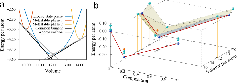
Figure 1: (a) A schematic energy-volume ($V$–$E$) diagram with three phases and their EOSs, each represented by a parabola. The negative slope of the common tangent to two adjacent EOS (solid black line) represents the pressure at which the two phases are in equilibrium. The LAE approximates the common tangent with a line connecting the ambient-condition equilibrium volumes/energies of two adjacent phases (solid grey line connecting filled grey circles). (b) A schematic $N$–$V$–$E$ convex hull for a model binary system. Individual phases are represented by spheres, and convex hull boundaries are indicated with solid red and dotted black lines. On the left is the conventional zero-pressure $N$–$E$ hull, a projection of the extended $N$–$V$–$E$ convex hull on the right. Phases that are thermodynamically stable at zero pressure lie on the $N$–$E$ convex hull (blue spheres). Metastable phases that are stable at some non-ambient pressure lie above the $N$–$E$ hull but on the $N$–$V$–$E$ convex hull (teal spheres). A phase that is truly unstable at any pressure lies above the $N$–$V$–$E$ hull (orange sphere).

The above linear approximation to enthalpy (henceforth referred to as “LAE”) is illustrated in an energy-volume diagram in Fig. 1a, where the ground state and two metastable states are each represented by their respective equation of states (EOS) $E(V)$, i.e., their energy as a function of volume, approximated by parabola. The negative slopes of the common tangents connecting the EOS of neighboring phases represent the pressure at which both phases are in equilibrium (“transition pressures”, black solid lines). With our approximation of the bulk moduli $B(p_{0})\to\infty$, the EOS curve of each phase would have infinitely large curvature, reducing the parabola to a vertical line originating at the corresponding equilibrium volumes $V_{0}$ and energies $E_{0}$. Essentially, all information of each phase is then contained in a single point at ($V_{0}$, $E_{0}$), represented by filled points.

Although the LAE is rather crude, it is reasonably accurate up to pressures in the range of tens, or even hundreds of GPa. As we will show in the rest of this work, the LAE can be used as a powerful tool to enable quick analyses of phase stability of a large number of materials at non-ambient pressures. Note that we will hereafter use the terms “zero pressure” and “ambient pressure” interchangeably, since the $pV$ contribution to the free energy at atmospheric pressure is insignificant for most inorganic compounds. E.g., at one atmosphere, which corresponds to roughly 1 bar, the energy contribution of $pV$ in diamond silicon with a volume of $\sim$20 Å³/atom is merely 0.012 meV/atom, far smaller than the error bars encountered in DFT calculations.

I.2 Thermodynamic stability: the convex hull

The thermodynamic stability of a phase at zero temperature can be determined by the construction of the so-called convex hull of all phases in the chemical space. At zero pressure, the convex hull is constructed from the composition and formation energy (composition-energy hull, or simply “$N$–$E$ convex hull”) of all the phases. By definition, a phase on the convex hull has a formation energy lower than that of any other phase (or linear combination of phases) at that composition, and is therefore thermodynamically stable. At non-ambient pressures, thermodynamic stability is determined by a convex hull which also takes into account the energy as a function of volume of all phases, given by their respective EOS $E(V)$. The LAE introduced in Section I.1 allows us to simplify the construction of the convex hull by taking into account the ambient volume of each phase, in addition to their composition and formation energy (compositon-volume-energy hull, or simply “$N$–$V$–$E$ convex hull”). A phase on the extended $N$–$V$–$E$ hull has a formation energy lower than any other phase or combination of phases at that composition and volume, and is therefore thermodynamically stable at some pressure. Further, a tie line on the convex hull represents a two-phase equilibrium, a triangular facet represents a three-phase equilibrium, and so on—a facet with $n$ vertices represents an $n$-phase equilibrium.

A schematic $N$–$V$–$E$ convex hull is shown in Fig. 1b. A projection of the extended $N$–$V$–$E$ convex hull taking into account only the energy and volumes leads to the $N$–$E$ hull (indicated by solid red lines). Phases that lie above the $N$–$E$ hull, but on the $N$–$V$–$E$ hull, are metastable at zero pressure but thermodynamically stable at some finite pressure. For example, in Fig. 1b, only two elemental phases and one binary compound (blue spheres) lie on the $N$–$E$ hull (solid red lines), i.e., are thermodynamically stable at zero pressure, and all other phases are metastable. However, all elemental phases and all binary compounds except one lie on the extended $N$–$V$–$E$ hull (teal spheres connected by dotted black lines), i.e., are thermodynamically stable at some non-ambient pressure. Only one phase shown (orange sphere at composition 0.2) is truly unstable at all pressures.

I.3 Pressure range of stability

For a system in thermodynamic equilibrium at zero temperature, $dE=-p\,dV+\sum_{i}\mu_{i}\,dN_{i}$, where $dE$, $dV$ are infinitesimal changes in internal energy $E$, volume $V$ of the system, respectively, and $dN_{i}$ is the infinitesimal change in the composition $N_{i}$ of species $i$. The equilibrium pressure is thus given by $p=-\left(\frac{\partial E}{\partial V}\right)_{N_{i}}$, i.e., the derivative of energy with respect to volume at constant composition. Hence, the pressure range of stability of a phase $\mathcal{P}$ with ambient equilibrium volume and energy of $V_{0}$ and $E_{0}$, respectively, is governed by the phase equilibria at volumes $(V_{0}+dV)$ and $(V_{0}-dV)$ . In other words, the window of pressures [$p_{-}$, $p_{+}$] where $\mathcal{P}$ is stable is given by

$$p_{\pm}=-\frac{E_{0}-E(V_{0}\mp dV)}{dV}$$ (3)

$E(V_{0}\pm dV)$ can be calculated by minimizing the free energy of the system at the target composition and volume. Grand canonical linear programming (GCLP) (32) techniques using efficient linear solvers are routinely employed to calculate phase stabilities and equilibrium reaction pathways at 0 K and 0 GPa (33; 34; 35; 36; 37). In this work, in addition to the average composition of the system being constrained to that of $\mathcal{P}$, the volume is constrained to $V_{0}\pm dV$ during energy minimization. Thus, a pressure range of stability can be calculated for every phase that lies on the extended $N$–$V$–$E$ convex hull.

As discussed in Sec. I.1, the negative slope of the common tangent to the EOS of two phases is the pressure at which the respective phases coexist, or in other words, one phase transforms into the other under the effect of pressure. In the LAE, the common tangent is reduced to a line connecting the local minima of the two phases (solid gray line connecting filled grey circles in Fig. 1a). The LAE introduces errors compared to the real transition pressure, which depend on the overall features of the energy landscape. If we assume that all phases are compressible with identical, finite bulk moduli, the LAE will consistently lead to an underestimation of the magnitude of the transition pressures. In practice, however, high-pressure phases often exhibit shorter, stronger bonds that lead to higher bulk moduli. Hence, the LAE would lead to a better agreement with the real transition pressures for phases stable at very high pressures. On the other hand, if the bulk moduli significantly decreased with pressure, the LAE would lead to an overestimation of the magnitude of the transition pressures. We also note that transition pressures, based on the above definition, can be positive or negative (e.g., the common tangents connecting the ground state with metastable phases 1 and 2, respectively in Fig. 1a). A negative pressure can be physically interpreted as a tensile stress, leading to the expansion of a phase toward volumes exceeding its ambient ground state equilibrium volume.

II Results and Discussion

II.1 Model validation

We first evaluate the accuracy of the linear approximation to enthalpy by investigating two elements and three binary systems in detail.

II.1.1 Elemental solids

We choose two elements whose high-pressure phase diagrams are among the most complex as well as the most well-studied: silicon and bismuth. Both elements have intricate energy landscapes with several high-pressure allotropes.

a. Silicon

The phase diagram of silicon has been well explored experimentally, partially due to its importance in the semiconductor industry. The ambient ground state is Si-I, which crystallizes in a cubic diamond structure (38). It transforms around 11 GPa to the Si-II phase, which has a $\beta$-Sn structure (39). This is followed by a transformation to Si-XI with $Imma$ symmetry (40) at 13 GPa. Above 16 GPa, Si-V forms in the simple hexagonal structure (41), and at 38 GPa, Si-VI forms in an orthorhombic $Cmcm$ structure (42). The hexagonal close-packed Si-VII forms above 42 GPa (43), and finally, cubic close-packed Si-X forms at pressures above 78 GPa (44).

We first compute the pressure range of stability of the various silicon allotropes using DFT calculations (see the top panel labeled “Exact” in Fig. 2(a)). For each phase, we calculate the enthalpy explicitly at various pressures at intervals of 2 GPa and 10 GPa in the range of 0–20 GPa and 20–100 GPa, respectively. The transition pressures are then computed by minimizing the interpolated formation enthalpies as a function of pressure. The experimentally reported sequence of formation and transition pressures of high-pressure Si allotropes are well reproduced, with the exception of Si-II, which is effectively degenerate in enthalpy to Si-XI. The discrepancy between experiment and theory for the transition from Si-I to Si-II has been well studied (45; 46), and is attributed to the errors associated with the PBE approximation to the DFT exchange correlation potential.

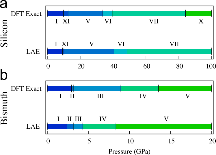
Figure 2: The pressure range of stability of high-pressure phases of elemental (a) silicon and (b) bismuth, respectively. Explicitly computed transition pressures using DFT-calculated formation enthalpies are labeled “DFT Exact” (top bar in each panel), and those based on the LAE are denoted with “LAE” (bottom bar in each panel). The crystal structures of the silicon and bismuth allotropes were taken from the Refs. 38; 39; 40; 41; 42; 43; 44 and 47; 48; 49; 50; 51; 52; 53, respectively.

We then calculate the pressure range of stability of all the allotropes using only the respective equilibrium energies and volumes at 0 GPa, extrapolated linearly as described in Sections I.1–I.3 (see the bottom panel labeled “LAE” in Fig. 2a). The agreement between the “DFT Exact” and “LAE” phase diagrams is remarkable: (a) the sequence of the phases is correctly reproduced, with the only exception of Si-X, which the linear approximation model predicts to be unstable even at 100 GPa, and (b) the overall errors in the transition pressures predicted by the approximate model are within around 10% of those calculated explicitly.

b. Bismuth

At ambient condition, bismuth crystallizes in a rhombohedral Bi-I phase with space group $R\bar{3}m$. It transforms at a pressure of around 2.55 GPa to Bi-II with a $C2/m$ structure (47; 48) and a very narrow range of stability at low temperatures. Upon increasing the pressure, Bi-III forms in a complicated, incommensurate host-guest structure with $P4/ncc$ symmetry (49; 50; 51). A Bi-IV phase with space group $P21/n$ has been reported between 2.4 GPa and 5.3 GPa at temperatures above around 450 K (52). Finally, the Bi-V bcc phase is observed at pressures above 7.7 GPa (53).

Similar to the case of silicon, we first compute the pressure range of stability of the various bismuth allotropes using enthalpies calculated explicitly at various pressures at intervals of 1 GPa in the range of 0–20 GPa (see the top panel labeled “DFT Exact” in Fig. 2b). Although the experimentally reported sequence of allotropes formed is well reproduced, the transition pressures between Bi-III/Bi-IV and Bi-IV/Bi-V are severely overestimated. This behavior has been reported previously by Häussermann et al. (51), and corroborated in our recent work on Cu–Bi intermetallics (54; 55).

The pressure range of stability of all allotropes calculated using the LAE reproduces the correct sequence of formation (see the bottom panel labeled “LAE” in Fig. 2b). However, the agreement between the transition pressures predicted by the approximate model and those calculated explicitly are worse than that for silicon allotropes. We attribute these larger errors to the strong changes in the chemical bonds between the different bismuth phases, especially since ambient Bi-I has a layered structure, in contrast to the high-pressure phases. Hence, our approximation of equal, infinitely large bulk moduli for every phase is perhaps less reasonable for elemental phases of bismuth.

II.1.2 Binary intermetallics

When compared to pure elements, the high-pressure phase space of binary/higher-order chemical systems have been experimentally relatively unexplored. Including composition and pressure as additional degrees of freedom significantly increases the complexity of the phase space. In this section, we focus on a unique subset of chemistries: intermetallic systems of elements that are not miscible at ambient conditions but form compounds under pressure. Many of these so-called ambient-immiscible systems involve bismuth in combination with other elements. Recently, we investigated three such systems in detail, namely Fe–Bi (56), Cu–Bi (54; 55), and Ni–Bi (57), by performing extensive global structure searches. Here, we use these three systems to further evaluate the performance of the linear approximation to enthalpy.

a. Fe–Bi
Using the minima hopping crystal structure prediction method (MHM), we recently predicted a high-pressure FeBi2 phase with I4/mcm symmetry at pressures above 36 GPa (56), which was experimentally confirmed through evidences found in the in-situ X-ray diffraction pattern at above 30 GPa (10). We note that the discovery of FeBi2 resulted from extensive MHM structural searches performed at pressures of 0, 50 and 100 GPa. The most promising candidate structures were then relaxed at pressure intervals of 10 GPa to compute enthalpies, which were in turn used to calculate the pressure range of stability of various phases (see top panel in Fig. 3a). Besides the FeBi2 I4/mcm phase, we find a FeBi3 phase with the Cmcm symmetry to be stable in a very small pressure window slightly below 40 GPa. This phase has so far not been observed in experiment.

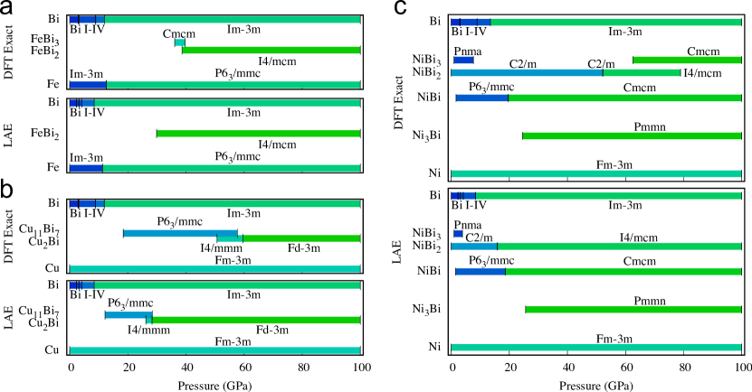
Figure 3: Comparison between the explicitly computed phase diagrams with the ones derived from the LAE model for binary systems. The panels (a), (b) and (c) correspond to the Fe–Bi, Cu–Bi and Ni–Bi systems, respectively. Explicitly calculated transition pressures using DFT are denoted with “DFT Exact” (top bar), and results based on the LAE are denoted with “LAE” (bottom bar).

We now compare the pressure range of stability calculated explicitly above against that calculated using the linear approximation to enthalpy, using only the ambient equilibrium energies and volumes of the phases. The phase diagram predicted by the approximate model (bottom panel in Fig. 3a) is qualitatively similar to the exact one: the FeBi2 I4/mcm phase becomes stable at comparable pressures. This finding can be conveniently exploited in structural searches: since the MHM samples many low-lying metastable structures at a fixed pressure $p_{0}$, one could use the energies and volumes at $p_{0}$ of such phases within the LAE to quickly predict if any of the metastable phases become stable at a different pressure $p\neq p_{0}$. Even for immiscible systems at $p_{0}$, potential candidate structures are found if the simulation cells are sufficiently small to prevent phase segregation. This means that a structural search conducted solely at 0 GPa might have been sufficient to uncover the I4/mcm structure and correctly predict the experimentally observed FeBi2 phase. The FeBi3 phase, on the other hand, with the narrow pressure window of stability is predicted to be unstable at all pressures by the approximate model; this could be a result of errors associated with DFT calculations. The good agreement between the exact and approximate phase diagrams is rather surprising: FeBi2 undergoes a series of magnetic transitions between 0 and 40 GPa, accompanied by abrupt changes in the unit cell volume (56), all of which are neglected in the linear approximation to enthalpy.

b. Cu–Bi

In the ambient-immiscible Cu–Bi system, at least two compounds, with compositions Cu11Bi7 and CuBi, have been recently discovered in DAC experiments between 3 and 6 GPa (54; 55). Both phases can be recovered to ambient conditions, and exhibit exciting superconducting and structural properties. For example, CuBi has a layered structure, rather uncommon for high-pressure phases, and is calculated to have an extremely low energy cost associated with exfoliation from bulk into single sheets (58). Further, more recent structural searches predict additional, dense Cu2Bi phases to become thermodynamically accessible at pressures of above 50 GPa (59).

The top panel in Fig. 3b shows the pressure range of stability of the various high-pressure Cu–Bi phases computed using explicitly calculated enthalpies for each phase. The CuBi phase is not thermodynamically stable at any pressure at zero temperature, consistent with recent reports of vibrational entropy playing a crucial role in rendering this phase synthesizeable (55). The Cu11Bi7 phase is thermodynamically accessible at high pressures up to around 60 GPa, when it starts to compete with two dense Cu2Bi phases (59).

The bottom panel in Fig. 3b shows the Cu–Bi phase diagram computed from the LAE, using only the respective equilibrium energy and volume of each phase at 0 GPa. All phases are correctly predicted to be stable by the approximate model, consistent with the exact phase diagram. As expected, the transition pressures predicted by the approximate model are underestimated overall when compared to those calculated explicitly—a trend that is presumably increased due to the significant structural changes in elemental bismuth as a function of pressure (see Section II.1.1). Nonetheless, it is striking that, using the simple linear approximation to enthalpy, we could have correctly predicted all the high-pressure phases in the Cu–Bi system from a structural search only at 0 GPa.

c. Ni–Bi

We tested for the first time the predictive power of our model by investigating the high-pressure phases in the Ni–Bi binary intermetallic system. Two compounds have been experimentally reported at ambient pressures: NiBi in the hexagonal NiAs structure (60), and NiBi3 in the orthogonal RhBi3 structure (61; 62). Both compounds are superconductors with transition temperatures of $4.25\text{\,}\mathrm{K}$ and $4.06\text{\,}\mathrm{K}$ in NiBi (63) and NiBi3 (64; 65), respectively. To generate phase data to be used within the LAE to construct the convex hull and predict transition pressures, we used prototypes from our previous structural searches of the Fe–Bi and Cu–Bi systems, and substituted the Fe/Cu sites with Ni atoms, followed by structural relaxation at ambient pressures. Using this ambient-pressure dataset of energies and volumes, the LAE model predicted stable compounds at high-pressure for the compositions Ni3Bi and NiBi2. Based on this prediction, we performed a thorough investigation of the Ni–Bi system using MHM simulations at pressures of 10 and 50 GPa, which indeed revealed a number of high-pressure phases.

In particular, our calculations predict new compounds stable at high-pressure at compositions of the previously reported ambient-pressure phases, i.e., NiBi and NiBi3. The hexagonal $\alpha$-NiBi phase undergoes a structural transition to a TlI-type structure with $Cmcm$ symmetry at pressures above around 20 GPa. Similarly, the orthorhombic NiBi3 phase is thermodynamically unstable above 7.5 GPa, and a $Cmcm$ structure is stable above 62 GPa. Further, we discover additional stable phases at previously unexplored compositions. We find that a NiBi2 phase with $C2/m$ symmetry in the PdBi2 structure type is in fact thermodynamically stable at ambient pressures, a finding that was reported earlier by Bachhuber et al. (66). At the same composition, a second $C2/m$ phase becomes stable above 52 GPa, over a very small pressure window of less than 1 GPa, followed by a $I4/mcm$ phase, isostructural to FeBi2. Finally, a Ni3Bi compound with $Pmmn$ symmetry, isostructural to Ni3Sb in the Cu3Ti structure type, is predicted to be stable at pressures above 25 GPa.

One of our predictions was very recently verified by compressing NiBi in a diamond anvil cell (DAC). Heating to temperatures above 700^∘C at pressures above $\approx 28$ GPa, the hexagonal $\alpha$-NiAs transforms into $\beta$-NiAs in the predicted TlI structure type (57). The experimental transition pressure is somewhat higher than the calculated value of 20 GPa. This discrepancy could be attributed to the presence of high kinetic reaction barriers in the first-order phase transition, which requires heat to induce the phase change and inevitably leads to calculated transition pressures being lower than those observed in experiment. This hypothesis is supported by detectable evidences of the $\beta$-NiAs phase in the XRD pattern upon decompression: the $\beta$-NiAs is kinetically persistent as low as 11.62 GPa, hence the equilibrium pressure lies anywhere between 11.62 and 28.3 GPa. In addition, errors inherent to the approximations used in DFT calculations could also explain the difference in the observed and computed transition pressures. The approximations to the exchange correlation potential alone can make a noticeable difference. E.g., the PBE functional predicts that both the experimentally observed NiBi and NiBi3 phases (in their reported structures) are not thermodynamically stable at 0 GPa and 0 K. However, we find that LDA correctly places the two experimental phases on the 0 GPa convex hull, and if we additionally take into account the vibrational entropy contributions to the free energy, NiBi2 becomes unstable at elevated temperatures. A detailed investigation of the influence of different exchange correlation potentials and temperature effects on the calculated phase stability of Ni–Bi compounds and their properties will be reported elsewhere.

After exploring the high-pressure Ni–Bi system with the MHM, we a posteriori compare the phase diagram of Ni–Bi computed using the explicitly calculated enthalpies against that predicted from our LAE model (Fig. 3c), and find remarkable agreement. Most phases, and the sequence in which they form under pressure, are correctly predicted by the approximate model. The only exceptions are the $Cmcm$ phase at the NiBi3 composition and the second $C2/m$ compound at the NiBi2 composition at around 50 GPa. As discussed earlier, the latter phase has a very small pressure range of stability of $<$1 GPa, so its absence in the phase diagram predicted by the approximate model is not surprising. In fact, similar to the $Cmcm$ FeBi3 phase that was predicted to be stable in a narrow pressure window of less than 3 GPa but not yet observed experimentally, synthesis of the NiBi2 phase is likely to be challenging, if possible at all.

II.2 Large-scale analysis of phase stability at high pressure

II.2.1 Elements and binary compounds

The power of our linear enthalpy model lies in its capability to efficiently assess the pressure range of stability of hundreds of thousands of phases. Since the linear approximation requires only equilibrium energies and volumes of phases calculated at ambient pressure, it can be used to leverage the large materials datasets available in HT-DFT databases such as the OQMD (22; 23), Materials Project (24), and AFLOWlib (25). Here, we present large-scale analysis and statistics of thermodynamic phase stability of materials at high pressure using ambient-pressure phase data calculated in the OQMD.

First, we focus on elemental high-pressure phases, and begin by compiling a “validation-dataset” of experimentally reported high-pressure elemental phases. The crystal structures of many high-pressure phases reported in the Inorganic Crystal Structure Database (ICSD) (27) have been calculated in the OQMD, albeit at ambient pressure. For every element, we filter all entries in the ICSD using the “External Conditions $\rightarrow$ Pressure” metadata available for each entry. Further, Tonkov et al. (67) compiled a comprehensive list of phase transformations under pressure for nearly 100 elements, on which we rely heavily as a second reference to cross-validate and augment the list of high-pressure phases calculated in the OQMD. Our final compiled dataset contains 132 distinct elemental high-pressure phases, and can be found in the Supplementary Materials (SM).

For each element in the periodic table, we use the ambient-pressure energy and volume data for all ICSD phases (i.e., not limited to high-pressure phases) calculated in the OQMD within the LAE model to predict (a) the number of phases from our validation-dataset that lie on the extended $N$–$V$–$E$ convex hull, i.e., the number of phases stable at some finite pressure, and (b) the pressure range of stability of every phase that lies on the $N$–$V$–$E$ hull. Fig. 4 shows a summary of this analysis in the form of a periodic table: for every element with at least one experimentally reported high-pressure phase, we indicate the number of high-pressure phases in our compiled dataset from the OQMD (bottom-left half) and the number of phases predicted by the linear enthalpy model to lie on the $N$–$V$–$E$ hull (top-right half), represented on a color scale. That is, the number of phases reported experimentally and those predicted to be stable at some finite-pressure match exactly whenever the colors in both the left and right segments are identical. This is indeed the case for most elements, with a few exceptions. Overall, 75% of all experimentally reported high-pressure phases are predicted to lie on the $N$–$V$–$E$ convex hull (see the top panel of Table 1). In addition, for around 35% of the phases, the predicted pressure range of stability overlaps with the respective transition pressures reported in experiment. The low success rate in correctly predicting the transition pressure is somewhat expected following the model validation on Si and Bi in Section II.1. We discuss the possible sources of discrepancy between predictions and experiment toward the end of this Section.

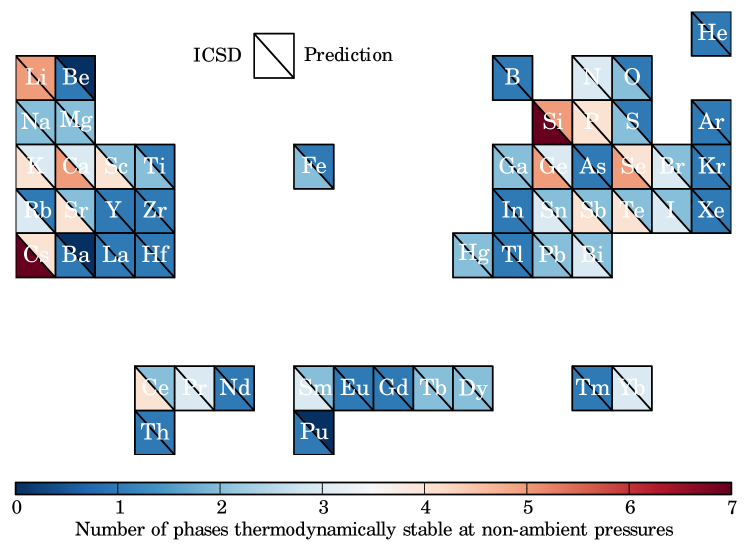
Figure 4: Comparison of predictions of high-pressure elemental phases from the LAE model against experiment. For each element, the number of (a) unique phases reported experimentally and (b) predicted by the linear enthalpy model to be thermodynamically stable at non-ambient pressures, are indicated by the color of the bottom-left and top-right halves, respectively, of the corresponding tile in the periodic table. Overall, the model correctly predicts $\sim$75% of the high-pressure phases in the ICSD to be thermodynamically stable at non-ambient pressures.

Next, we perform a similar large-scale analysis for all experimentally reported binary phases. Using calculations of experimentally reported compounds in the OQMD, curated using pressure-related metadata in the ICSD (in a manner similar to that employed for elemental phases), we compile a dataset of 343 unique binary compounds in total as a validation-dataset (the entire list is available in Supplementary Materials). This number is significantly lower than that expected from a simple combinatorial estimation. For elemental solids, we found in average more than one high-pressure phase per element. If we extend this observation to binaries and assume that every binary system has in average more than one high-pressure phase, the number of potential high-pressure phases considering 90 elements is ${}^{90}{\rm C}_{2}=4005$. We note that our estimation is very conservative, since binary $A$–$B$ systems introduce an additional, compositional degree of freedom, which allows multiple high-pressure phases to exist at the same pressure, A_pB_q, as we have seen in Sec. II.1.2. This indicates that the high-pressure phase diagrams of binary systems in general have been relatively underexplored. The linear enthalpy model performs equally well for binary compounds — 80% of experimentally reported high-pressure binary phases are predicted to be stable at some finite pressure (see lower panel of Table 1). For around 35% of the phases, the predicted pressure range of stability overlaps with the respective transition pressures reported experimentally.

Table 1: Accuracy of the linear enthalpy model in predicting the stability (at some finite-pressure) of experimentally reported elemental and binary high-pressure phases.

Elements
Experimentally reported HP phases	132
Predicted to be stable at finite pressure	97 (75%)
Predicted pressure range of stability	45 (35%)
matches experiment
Binaries
Experimentally reported HP phases	343
Predicted to be stable at finite pressure	273 (80%)
Predicted pressure range of stability	125 (35%)
matches experiment

Overall, our “crude” linear enthalpy model performs surprisingly well, with a success rate of 75–80%, in predicting the stability of both elemental and binary high-pressure phases. We identify four potential sources of error that could explain the discrepancy between the number of high-pressure phases reported experimentally and that predicted by our approximate model:

1. The crystal structure reported experimentally for the phase is erroneous. Resolving the crystal structure, e.g., from in-situ XRD measurements, under high pressure is a difficult and tedious task that can lead to incomplete/incorrect structural characterization. A prominent example is the Bi-III phase, the crystal structure of which was experimentally resolved only after several failed attempts (49). In fact, Bi-III has an incommensurate host-guest structure and the reported structure is only a representative ordered model with $P4/nnc$ symmetry (51). A similar incommensurate structure has been reported for phase IV of phosphorus in the pressure range of 107-137 GPa (68).

2. The high-pressure phase emerges via a phase transition of second order. In this case, the structural relaxations performed using DFT will inevitably transform the high-pressure phase to a lower-pressure structure. Therefore, our linear enthalpy model, which relies on the equilibrium energy $E_{0}$ and volume $V_{0}$ at ambient pressure of a high-pressure phase, will expectedly not capture its stability.

3. Errors inherent to DFT calculations and numerical noise, e.g., due to the approximation to the exchange correlation potential, pseudization of core electrons (which might be important especially at high pressures), unconverged basis sets and sampling meshes, insufficient tolerances during structural relaxations, etc.

4. Finally, there is the inherent error due to applying a linear approximation to the enthalpy of each phase (i.e., assuming all phases to be perfectly incompressible), which might be unreasonable for some materials at large values of pressure.

II.2.2 All experimentally reported compounds

We now use our linear enthalpy model to analyze the phase stability of all experimentally reported compounds calculated in the OQMD (not limited to high-pressure phases), a total of around 33,000 unique ordered compounds. As earlier, using the equilibrium energy and volume at ambient pressure of each phase in our dataset, we predict the number, and the pressure range of stability, of all phases that lie on the extended $N$–$V$–$E$ convex hull (i.e., presumably thermodynamically stable at some finite-pressure).

First, we find that only around 55% of the 33,000 compounds in our dataset lie on the $N$–$E$ convex hull, i.e., are thermodynamically stable at ambient pressure conditions, consistent with a previous report on a similar dataset from the OQMD (23). A recent study by Sun et al.(6) on a dataset of 29,900 experimentally reported compounds calculated in the Materials Project also finds around 50$\pm$4% of the phases to be ambient-metastable. In the latter study, it is proposed that the observed metastable compounds are generally remnants of thermodynamic conditions where they were once the stable ground states.

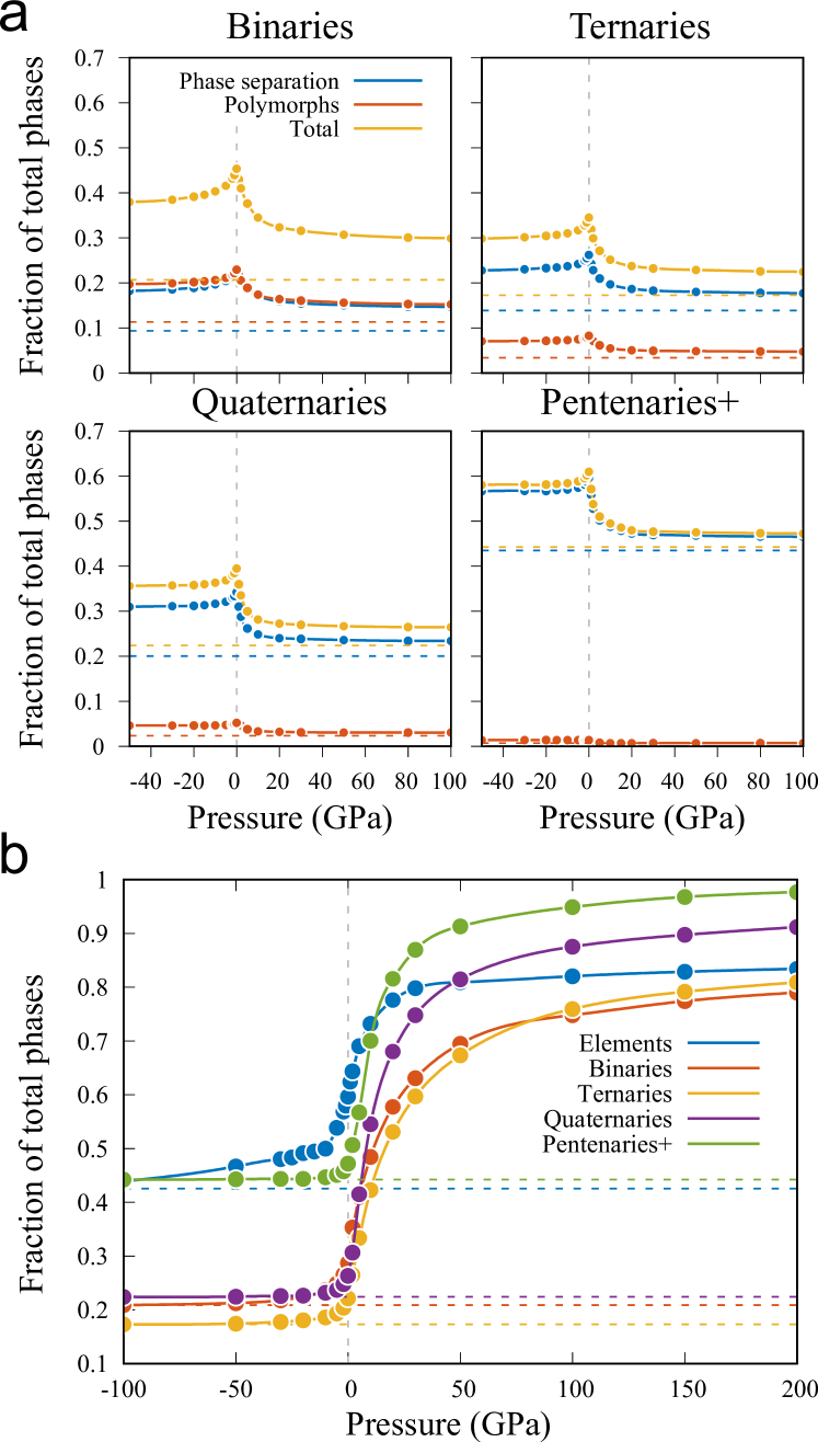
Figure 5: (a) Fraction of metastable phases that become thermodynamically stable with incremental increase/decrease in pressure, with respect to 0 GPa. The horizontal dashed lines indicate the fraction of metastable phases that do not lie on the $N$–$V$–$E$ convex hull at any pressure. (b) Fraction of ambient-metastable phases that cannot be accessed thermodynamically at any pressure larger than pressure $p$, equivalent to $1-$ (fraction of phases that can be accessed at some pressure larger than pressure $p$).

We next test this hypothesis of “remnant metastability” by using pressure as a thermodynamic handle and tracking the number of metastable phases that become stable with incremental increase/decrease in pressure, with respect to ambient conditions. Fig. 5a shows the fraction of metastable phases as a function of positive (compressive) or negative (tensile) pressure, separated into binary, ternary, quaternary and higher-component systems. We observe a range of trends based on our statistical analysis.

First of all, the number of metastable phases decreases with incremental application of both positive and negative pressures, relative to 0 GPa. In other words, a significant fraction of the ambient-metastable phases are in fact thermodynamically stable ground states at non-ambient pressure conditions. For example, in the case of binary compounds (top left in Fig. 5a), the fraction of metastable phases decreases from around 0.45 at 0 GPa to around 0.30 at 100 GPa—15% of the ambient-metastable phases are rendered thermodynamically stable at some pressure $p\in(0,100]$ GPa. However, in each case, a sizeable fraction of metastable phases remain metastable at all pressures, i.e., they are not equilibrium ground states at any pressure (represented by horizontal dashed lines in Fig. 5a). For example, around 21% of all binary ambient-metastable phases cannot be accessed thermodynamically via pressure alone.

Second, the rate of decrease in the number of metastable phases (or increase in the number of metastable phases made stable) with pressure is maximum near zero and decays rapidly toward higher positive/negative pressures. This is most likely due to a bias toward small values of pressure in our compiled set of phases—after all, most compounds reported experimentally are likely observed in near-ambient conditions—but could be also due to a fundamental property of materials, namely, the density of stable ground states as a function of volume/pressure is maximum near zero pressure.

Third, we find considerable differences concerning the “character” of metastability in binary, ternary, and higher order compositional systems. We distinguish two subsets for each $n$-component dataset ($n=$ 2, 3, 4, $\geq$5)—“polymorphs” and “phase separation”—depending on whether a given phase is metastable with respect to another phase at the same composition or a combination of phases, respectively, at ambient conditions. We note that the higher the number of components present in a metastable compound, the more likely it is to phase-separate rather than transform into a polymorph, in agreement with previous observations (6). Further, the lower the number of components in a metastable compound, the more likely it is to be stabilized with pressure. Considering the subset of all metastable phases that phase-separate at ambient pressure, 58%, 47%, 42%, and 27% become thermodynamically stable at some finite positive/negative pressure in the case of binary, ternary, quaternary, and higher-component systems, respectively.

Additionally, we observe that the effects of positive and negative pressures on the metastability of phases are not symmetric about zero pressure: a much larger portion of ambient-metastable phases become thermodynamically stable under positive (compressive) pressure when compared to negative (tensile) pressure. A difference is perhaps expected considering that the limiting behaviors are very different: large positive pressures favor the formation of close-packed phases before eventual overlap of atomic cores, while the limit of large negative pressures is simply the individual non-interacting atoms of each species in the phase.

Finally, we probe a complementary question: if one were to incrementally tune external conditions from large positive to large negative pressures, how many observed metastable phases $\mathcal{N}$ can be accessed thermodynamically below any given pressure $p$? We calculate at pressure $p$, the number of experimentally observed phases from our dataset that cannot be thermodynamically accessed at any pressure $>p$. We present this data as a cumulative histogram of the fraction of phases, integrated from pressures $p$ to $+\infty$, separated into elements, binaries, ternaries, etc. in Fig. 5b. Hypothetically, if all experimentally reported compounds were thermodynamically stable ground states at some finite pressure, one would expect this cumulative fraction of unstable phases to be 1 and 0 for $p\to\infty$ and $p\to-\infty$, respectively. Consistent with our previous observations, we find that (a) a sizable fraction of the phases do not lie on the extended $N$–$V$–$E$ convex hull at all, i.e., they are not ground states under any pressure (represented by horizontal dashed lines in Fig. 5b), and (b) the rate at which additional metastable phases can be thermodynamically accessed is maximum near zero pressure (given by the slopes of the curves). In other words, the pressure density of thermodynamic ground states, $\frac{d\mathcal{N}}{dp}$, is maximum near $p=0$. Whether this is an artifact of using a dataset of experimentally observed phases or is a fundamental property of matter, needs further analysis, and will be the subject of future work.

II.3 Discovery of new high-pressure compounds

So far, we have used the LAE to analyze the phase stability of experimentally reported high-pressure elemental and binary phases, and to probe the accessibility of ambient-metastable phases using pressure as a thermodynamic handle. Now, we go a step further by using the LAE to predict new intermetallic compounds by combining it with CSP methods. For this purpose, we focus on a unique subset of binary systems, namely, the combination of elements that are immiscible at ambient pressures. According to the data we compiled from the OQMD, there currently exist $\sim$1780 binary systems that do not contain any experimentally observed compounds. Any high-pressure phases that we identify in these systems are therefore true predictions of new materials.

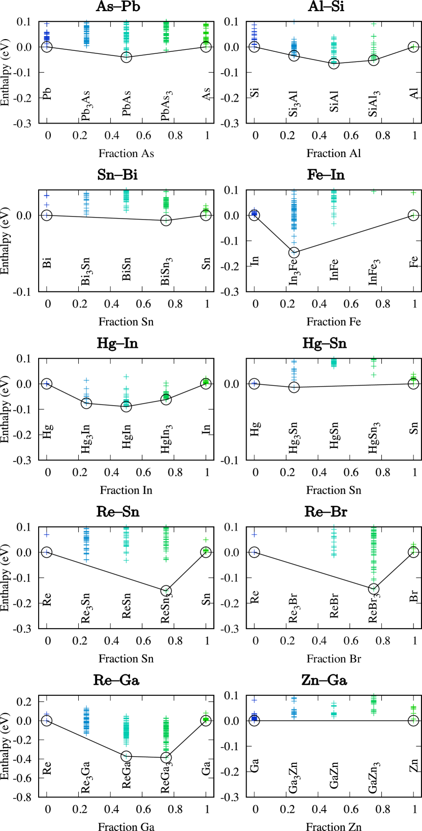
Figure 6: The convex hulls of formation enthalpy of ten ambient-immiscible binary systems calculated using structural search at 50 GPa via the MHM. Each cross denotes a phase sampled with the MHM. In all but the Zn-Ga system, we find at least one thermodynamically stable high-pressure phase.

For the dataset to be used for construction of the convex hull and calculation of transition pressures within the LAE, we use ambient-pressure formation energies and volumes of phases calculated in the OQMD. As mentioned in Section IV.1, the OQMD contains calculations of more than 450,000 compounds including experimentally reported compounds from the ICSD, and hypothetical compounds generated by decoration of common structural prototypes with all the elements in the periodic table. The Strukturbericht symbols of the prototype structures considered in this section are listed below (23; 69):

1. elemental prototypes: A1 (fcc), A2 (bcc), A3 (hcp), A3’ ($\alpha$-La), A4 (diamond), A5 ($\beta$-Sn), A7 ($\alpha$-As), A9 (graphite), A10 ($\alpha$-Hg), A11 ($\alpha$-Ga), A12 ($\alpha$-Mn), A13 ($\beta$-Mn), A_b ($\beta$-U), A_h ($\alpha$-Po), $C19$ ($\alpha$-Sm)

2. binary $AB$: B1 (NaCl), B2 (CsCl), B3 (zincblende ZnS), B4 (wurtzite ZnS), B19 (AuCd), B_h (WC), L1₀ (AuCu), L1₁ (CuPt)

3. binary $A_{3}B$: L1₂ (Cu₃Au), D0₁₉ (Ni₃Sn), D0₂₂ (Al₃Ti), D0₃ (AlFe₃)

We screen for promising chemical systems that contain high-pressure phases in the following manner: for every ambient-immiscible binary system, we use the LAE to predict the thermodynamic phase stability and pressure range of stability of each hypothetical compound in that chemical space. We select systems that contain at least one hypothetical compound predicted to become stable below an arbitrary pressure threshold of 50 GPa. We then rank these systems according to the predicted transition pressures, from lowest to highest, and select 10 of the most promising systems for further investigation. For each system, we further verify that no compound in that chemical space is reported in the ICSD or in phase diagrams available in the ASM Alloy Phase Diagram Database (70). At each composition where our model predicts a stable high-pressure phase we perform structural searches using the MHM, starting from the respective prototype structure from the OQMD, using simulation cells with up to 10 atoms/cell. Due to the set of binary prototypes currently calculated in the OQMD (see list above), the compositions we sample are limited to $A_{3}B$, AB and $AB_{3}$. Note that both the system size and the number of sampled compositions are far too low to give accurate predictions of the true high-pressure ground states. The structural searches are merely intended as proof-of-concept, i.e., to provide a sampling of configurations beyond the limited number of prototype structures.

Of the ten selected ambient-immiscible binary systems, namely, As-Pb, Al-Si, Sn-Bi, Fe-In, Hg-In, Hg-Sn, Re-Sn, Re-Br, Re-Ga, and Zn-Ga, structural searches performed at 50 GPa using the MHM confirmed the existence of at least one new stable high-pressure phase in all but the Zn-Ga system (see Fig. 6). All thermodynamically stable structures at 50 GPa are provided in the Supplementary Materials (SM). The high-pressure phases predicted present a number of avenues for experimental synthesis and verification. Overall, the success of the linear enthalpy model in guiding more accurate, sophisticated techniques based on crystal structure prediction in discovering novel high-pressure phases is remarkable.

III Conclusions

In summary, we present a method that allows an efficient screening for materials that are thermodynamically stable at non-ambient pressures using a simple linear approximation to the formation enthalpy of a phase. Using a generalized convex hull construction, the stability of thousands of compound can be evaluated at a low computational cost based on ambient-pressure data that is currently available in many materials databases without performing any additional DFT calculations. Through a large-scale analysis of experimentally reported compounds, we show that a large fraction of the observed ambient-metastable phases are in fact thermodynamic ground states at some finite pressure. Our method can be readily extended by further generalizing the convex hull construction and taking into account additional thermodynamic degrees of freedom, including temperature or surface areas of finite particles. Finally, we demonstrate the predictive power of this model when combined with a crystal structure prediction technique by discovering novel high-pressure phases in a set of ambient-immiscible binary intermetallic systems.

IV Methods

IV.1 Calculation of thermodynamic quantities

The equilibrium formation energy and volume data for all the phases considered in our analysis using LAE were retrieved from the Open Quantum Materials Database (OQMD) (22; 23). The dataset consists of DFT-calculated properties of over 450,000 compounds which include (a) unique, ordered experimentally reported compounds from the Inorganic Crystal Structure Database (ICSD), and (b) hypothetical compounds generated by the decoration of common structural prototypes with all the elements in the periodic table. Details of the settings used to calculate the equilibrium formation energy and volume of compounds in the OQMD can be found in Ref. 23.

All other DFT calculations reported in this work, i.e., those performed as part of global structure searches, were performed using the Vienna Ab initio Simulation Package (VASP) (71; 72; 73). We use the projector augmented wave (PAW) formalism (74; 75) and the PBE parameterization of the generalized gradient approximation to the exchange correlation functional (76) throughout. For all calculations, we use $\Gamma$-centered $k$-point meshes with about 8000 $k$-points per reciprocal atom and a plane-wave cutoff energy of 520 eV. All atomic and cell degrees of freedom of a structure are relaxed until the force components on all the atoms are within 0.01 eV/Å, and stresses are within a few kbar.

IV.2 Structural searches

The minima hopping method (MHM) (77; 78) implements a highly reliable algorithm to explore the low enthalpy phases of a compound at a specific pressure given solely the chemical composition (79; 80; 81). The low lying part of the enthalpy landscape is efficiently sampled by performing consecutive, short MD escape steps to overcome enthalpy barriers, followed by local geometry optimizations. The Bell-Evans-Polanyi principle is exploited through a feedback mechanism on the MD escape trials, and by aligning the initial MD velocities along soft-mode directions in order to accelerate the search (82; 83). The MHM has been successfully applied to identify the structure and composition of many materials, also for systems at high pressures (84; 85; 86; 56; 55; 59). In this work, we performed MHM simulations only at the compositions where a high-pressure phase is predicted to be stable by the linear enthalpy model.

IV.3 Software implementation

All convex hull constructions in this work were performed using the Qhull library (87) as implemented in the SciPy Python package (88). The GCLP calculations reported in this work were performed using the Cbc solver distributed with the PuLP Python library (89). An implementation of the framework described in Sections I.1–I.3 has been made available as an open-source Python module (90). An implementation of the MHM is available through the Minhocao package (77; 78).

V Acknowledgments

M.A. and V.I.H. conceived and carried out the project, and contributed equally to this work, S.D.J. and C.W. supervised the project, and all authors contributed to writing the manuscript. M.A. (construction of linear model, crystal structure prediction) acknowledges support from the Novartis Universität Basel Excellence Scholarship for Life Sciences and the Swiss National Science Foundation (Project No. P300P2-158407, P300P2-174475). V.I.H. (model implementation, high-throughput calculations) and C.W. acknowledge support from the Department of Energy, Office of Science, Basic Energy Sciences under Grant DE-SC0015106. S.D.J. acknowledges support from NSF DMR-1508577 and the Carnegie/DOE Alliance Center (CDAC). The authors acknowledge support from the Data Science Initiative at Northwestern University. The computational resources from the Swiss National Supercomputing Center in Lugano (Projects s499, s621, s700), the Extreme Science and Engineering Discovery Environment (XSEDE) (which is supported by National Science Foundation Grant OCI-1053575), the Bridges system at the Pittsburgh Supercomputing Center (PSC) (which is supported by NSF Award ACI-1445606), the Quest high performance computing facility at Northwestern University, and the National Energy Research Scientific Computing Center (DOE: DE-AC02-05CH11231), are gratefully acknowledged.

References

- Gibbs (1878) J. W. Gibbs, Am. J. Sci. Series 3 Vol. 16, 441 (1878).
- Rosenstein and Lamy (1969) S. Rosenstein and P. P. Lamy, Am. J. Hosp. Pharm. 26, 598 (1969).
- Brog et al. (2013) J.-P. Brog, C.-L. Chanez, A. Crochet, and K. M. Fromm, RSC Adv. 3, 16905 (2013).
- Gopalakrishnan (1995) J. Gopalakrishnan, Chem. Mater. 7, 1265 (1995).
- Stein et al. (1993) A. Stein, S. W. Keller, and T. E. Mallouk, Science 259, 1558 (1993).
- Sun et al. (2016a) W. Sun, S. T. Dacek, S. P. Ong, G. Hautier, A. Jain, W. D. Richards, A. C. Gamst, K. A. Persson, and G. Ceder, Sci. Adv. 2, e1600225 (2016a).
- Oganov (2010) A. R. Oganov, Modern Methods of Crystal Structure Prediction, 1st ed. (Wiley-VCH Verlag GmbH & Co. KGaA, 2010).
- Pickard and Needs (2011a) C. J. Pickard and R. J. Needs, J. Phys.: Condens. Matter 23, 053201 (2011a).
- Zhang et al. (2013) W. Zhang, A. R. Oganov, A. F. Goncharov, Q. Zhu, S. E. Boulfelfel, A. O. Lyakhov, E. Stavrou, M. Somayazulu, V. B. Prakapenka, and Z. Konôpková, Science 342, 1502 (2013).
- Walsh et al. (2016) J. P. S. Walsh, S. M. Clarke, Y. Meng, S. D. Jacobsen, and D. E. Freedman, ACS Cent. Sci. 2, 867 (2016).
- Zhang et al. (2017) L. Zhang, Y. Wang, J. Lv, and Y. Ma, Nat. Rev. Mater. 2, 17005 (2017).
- Amsler et al. (2015) M. Amsler, S. Botti, M. A. L. Marques, T. J. Lenosky, and S. Goedecker, Phys. Rev. B 92, 014101 (2015).
- Rasoulkhani et al. (2017) R. Rasoulkhani, H. Tahmasbi, S. A. Ghasemi, S. Faraji, S. Rostami, and M. Amsler, Phys. Rev. B 96, 064108 (2017).
- Wang et al. (2012) Y. Wang, M. Miao, J. Lv, L. Zhu, K. Yin, H. Liu, and Y. Ma, J. Chem. Phys. 137, 224108 (2012).
- Zhou et al. (2014) X.-F. Zhou, X. Dong, A. R. Oganov, Q. Zhu, Y. Tian, and H.-T. Wang, Phys. Rev. Lett. 112, 085502 (2014).
- Eivari et al. (2017) H. A. Eivari, S. A. Ghasemi, H. Tahmasbi, S. Rostami, S. Faraji, R. Rasoulkhani, S. Goedecker, and M. Amsler, Chem. Mater. 29, 8594 (2017).
- Chua et al. (2010) A. L.-S. Chua, N. A. Benedek, L. Chen, M. W. Finnis, and A. P. Sutton, Nat. Mater. 9, 418 (2010).
- Schusteritsch and Pickard (2014) G. Schusteritsch and C. J. Pickard, Phys. Rev. B 90, 035424 (2014).
- Lu et al. (2014) S. Lu, Y. Wang, H. Liu, M.-s. Miao, and Y. Ma, Nat. Commun. 5, 3666 (2014).
- Zhao et al. (2014) X. Zhao, Q. Shu, M. C. Nguyen, Y. Wang, M. Ji, H. Xiang, K.-M. Ho, X. Gong, and C.-Z. Wang, J. Phys. Chem. C 118, 9524 (2014).
- Fisicaro et al. (2017) G. Fisicaro, M. Sicher, M. Amsler, S. Saha, L. Genovese, and S. Goedecker, Phys. Rev. Materials 1, 033609 (2017).
- Saal et al. (2013) J. E. Saal, S. Kirklin, M. Aykol, B. Meredig, and C. Wolverton, JOM 65, 1501 (2013).
- Kirklin et al. (2015) S. Kirklin, J. E. Saal, B. Meredig, A. Thompson, J. W. Doak, M. Aykol, S. Rühl, and C. Wolverton, npj Computational Materials 1, 15010 (2015).
- Jain et al. (2013) A. Jain, S. P. Ong, G. Hautier, W. Chen, W. D. Richards, S. Dacek, S. Cholia, D. Gunter, D. Skinner, G. Ceder, and K. Persson, APL Mater. 1, 011002 (2013).
- Curtarolo et al. (2012) S. Curtarolo, W. Setyawan, S. Wang, J. Xue, K. Yang, R. H. Taylor, L. J. Nelson, G. L. W. Hart, S. Sanvito, M. Buongiorno-Nardelli, N. Mingo, and O. Levy, Comput. Mater. Sci. 58, 227 (2012).
- Curtarolo et al. (2013) S. Curtarolo, G. L. W. Hart, M. B. Nardelli, N. Mingo, S. Sanvito, and O. Levy, Nat. Mater. 12, 191 (2013).
- (27) “Inorganic Crystal Structure Database,” https://icsd.fiz-karlsruhe.de, [Online; accessed 20-September-2017].
- Shen and Mao (2017) G. Shen and H. K. Mao, Rep. Prog. Phys. 80, 016101 (2017).
- Tsuchiya (2013) J. Tsuchiya, Geophys. Res. Lett. 40, 4570 (2013).
- Pickard and Needs (2011b) C. J. Pickard and R. J. Needs, J. Phys.: Condens. Matter 23, 053201 (2011b).
- Note (1) This procedure is analogous to calculating the range of thermodynamic stability of a compound with respect to the chemical potential of a given species. Since the chemical potential of species , at , , is given by , the window of stability [, ] of the phase can be calculated using , i.e., as a perturbation of energy with respect to the composition of the species .
- R. Akbarzadeh et al. (2007) A. R. Akbarzadeh, V. Ozoliņš, and C. Wolverton, Adv. Mater. 19, 3233 (2007).
- Mason et al. (2011) T. H. Mason, X. Liu, J. Hong, J. Graetz, and E. H. Majzoub, The Journal of Physical Chemistry C 115, 16681 (2011).
- Aidhy et al. (2011) D. S. Aidhy, Y. Zhang, and C. Wolverton, Phys. Rev. B 84, 134103 (2011).
- Kirklin et al. (2013) S. Kirklin, B. Meredig, and C. Wolverton, Adv. Energy Mater. 3, 252 (2013).
- Emery et al. (2016) A. A. Emery, J. E. Saal, S. Kirklin, V. I. Hegde, and C. Wolverton, Chem. Mater. 28, 5621 (2016).
- Ma et al. (2017) J. Ma, V. I. Hegde, K. Munira, Y. Xie, S. Keshavarz, D. T. Mildebrath, C. Wolverton, A. W. Ghosh, and W. H. Butler, Phys. Rev. B 95, 024411 (2017).
- Dutta (1962) B. N. Dutta, Phys. Stat. Sol. (b) 2, 984 (1962).
- Jamieson (1963) J. C. Jamieson, Science 139, 762 (1963).
- McMahon and Nelmes (1993) M. I. McMahon and R. J. Nelmes, Phys. Rev. B 47, 8337 (1993).
- Hu and Spain (1984) J. Z. Hu and I. L. Spain, Solid State Commun. 51, 263 (1984).
- Hanfland et al. (1999) M. Hanfland, U. Schwarz, K. Syassen, and K. Takemura, Phys. Rev. Lett. 82, 1197 (1999).
- Olijnyk et al. (1984) H. Olijnyk, S. K. Sikka, and W. B. Holzapfel, Phys. Lett. A 103, 137 (1984).
- Duclos et al. (1987) S. J. Duclos, Y. K. Vohra, and A. L. Ruoff, Phys. Rev. Lett. 58, 775 (1987).
- Sun et al. (2016b) J. Sun, R. C. Remsing, Y. Zhang, Z. Sun, A. Ruzsinszky, H. Peng, Z. Yang, A. Paul, U. Waghmare, X. Wu, M. L. Klein, and J. P. Perdew, Nat. Chem. 8, 831 (2016b).
- Hennig et al. (2010) R. G. Hennig, A. Wadehra, K. P. Driver, W. D. Parker, C. J. Umrigar, and J. W. Wilkins, Phys. Rev. B 82, 014101 (2010).
- Brugger et al. (1967) R. M. Brugger, R. B. Bennion, and T. G. Worlton, Phys. Lett. A 24, 714 (1967).
- Akselrud et al. (2014) L. G. Akselrud, M. Hanfland, and U. Schwarz, Z. Kristallogr. - New Cryst. Struct. 218, 415 (2014).
- Chen et al. (1994) J. H. Chen, H. Iwasaki, T. Kikegawa, K. Yaoita, and K. Tsuji, in AIP Conference Proceedings, Vol. 309 (AIP Publishing, 1994) pp. 421–424.
- McMahon et al. (2000) M. I. McMahon, O. Degtyareva, and R. J. Nelmes, Phys. Rev. Lett. 85, 4896 (2000).
- Häussermann et al. (2002) U. Häussermann, K. Söderberg, and R. Norrestam, J. Am. Chem. Soc. 124, 15359 (2002).
- Chen et al. (1997) J. H. Chen, H. Iwasaki, and T. Kikegawa, J. Phys. Chem. Solids 58, 247 (1997).
- Aoki et al. (1982) K. Aoki, S. Fujiwara, and M. Kusakabe, J. Phys. Soc. Jpn. 51, 3826 (1982).
- Clarke et al. (2016) S. M. Clarke, J. P. S. Walsh, M. Amsler, C. D. Malliakas, T. Yu, S. Goedecker, Y. Wang, C. Wolverton, and D. E. Freedman, Angew. Chem. Int. Ed. 55, 13446 (2016).
- Clarke et al. (2017) S. M. Clarke, M. Amsler, J. P. S. Walsh, T. Yu, Y. Wang, Y. Meng, S. D. Jacobsen, C. Wolverton, and D. E. Freedman, Chem. Mater. 29, 5276 (2017).
- Amsler et al. (2017a) M. Amsler, S. S. Naghavi, and C. Wolverton, Chem. Sci. 8, 2226 (2017a).
- Powderly et al. (2017) K. M. Powderly, S. M. Clarke, M. Amsler, C. Wolverton, C. D. Malliakas, Y. Meng, S. D. Jacobsen, and D. E. Freedman, Chem. Commun. 53, 11241 (2017).
- Amsler et al. (2017b) M. Amsler, Z. Yao, and C. Wolverton, Chem. Mater. 29, 9819 (2017b).
- Amsler and Wolverton (2017) M. Amsler and C. Wolverton, Phys. Rev. Materials 1, 031801 (2017).
- Haegg and Funke (1929) G. Haegg and G. Funke, Z. Phys. Chem., Abt. B 6, 272 (1929).
- Glagoleva and Zhdanov (1954) V. P. Glagoleva and G. S. Zhdanov, Zh. Eksp. Teor. Fiz. 26, 337 (1954).
- Ruck and Söhnel (2006) M. Ruck and T. Söhnel, Z. Naturforsch. 61b, 785 (2006).
- Alekseevskii et al. (1952) N. Alekseevskii, N. Brandt, and T. Kostina, Izv. Akad. Nauk SSSR 16, 233 (1952).
- Alekseevskii (1948) N. Alekseevskii, Zh. Eksp. Teor. Fiz. 18, 101 (1948).
- Herrmannsdörfer et al. (2011) T. Herrmannsdörfer, R. Skrotzki, J. Wosnitza, D. Köhler, R. Boldt, and M. Ruck, Phys. Rev. B 83, 140501 (2011).
- Bachhuber et al. (2013) F. Bachhuber, J. Rothballer, T. Söhnel, and R. Weihrich, J. Chem. Phys. 139, 214705 (2013).
- Tonkov and Ponyatovsky (2004) E. Y. Tonkov and E. G. Ponyatovsky, Phase Transformations of Elements Under High Pressure, 1st ed. (CRC Press, Boca Raton, Fla, 2004).
- Fujihisa et al. (2007) H. Fujihisa, Y. Akahama, H. Kawamura, Y. Ohishi, Y. Gotoh, H. Yamawaki, M. Sakashita, S. Takeya, and K. Honda, Phys. Rev. Lett. 98, 175501 (2007).
- Kirklin et al. (2016) S. Kirklin, J. E. Saal, V. I. Hegde, and C. Wolverton, Acta Mater. 102, 125 (2016).
- Massalski et al. (1986) T. B. Massalski, H. Okamoto, P. Subramanian, L. Kacprzak, and W. W. Scott, Binary alloy phase diagrams, Vol. 1 (American Society for Metals, Metals Park, OH, 1986).
- Kresse and Hafner (1993) G. Kresse and J. Hafner, Phys. Rev. B 47, 558 (1993).
- Kresse and Furthmüller (1996a) G. Kresse and J. Furthmüller, Comput. Mater. Sci. 6, 15 (1996a).
- Kresse and Furthmüller (1996b) G. Kresse and J. Furthmüller, Phys. Rev. B 54, 11169 (1996b).
- Blöchl (1994) P. E. Blöchl, Phys. Rev. B 50, 17953 (1994).
- Kresse and Joubert (1999) G. Kresse and D. Joubert, Phys. Rev. B 59, 1758 (1999).
- Perdew et al. (1996) J. P. Perdew, K. Burke, and M. Ernzerhof, Phys. Rev. Lett. 77, 3865 (1996).
- Goedecker (2004) S. Goedecker, J. Chem. Phys. 120, 9911 (2004).
- Amsler and Goedecker (2010) M. Amsler and S. Goedecker, J. Chem. Phys. 133, 224104 (2010).
- Amsler et al. (2012a) M. Amsler, J. A. Flores-Livas, T. D. Huan, S. Botti, M. A. L. Marques, and S. Goedecker, Phys. Rev. Lett. 108, 205505 (2012a).
- Huan et al. (2012) T. D. Huan, M. Amsler, V. N. Tuoc, A. Willand, and S. Goedecker, Phys. Rev. B 86, 224110 (2012).
- Huan et al. (2013) T. D. Huan, M. Amsler, R. Sabatini, V. N. Tuoc, N. B. Le, L. M. Woods, N. Marzari, and S. Goedecker, Phys. Rev. B 88, 024108 (2013).
- Roy et al. (2008) S. Roy, S. Goedecker, and V. Hellmann, Phys. Rev. E 77, 056707 (2008).
- Sicher et al. (2011) M. Sicher, S. Mohr, and S. Goedecker, J. Chem. Phys. 134, 044106 (2011).
- Amsler et al. (2012b) M. Amsler, J. A. Flores-Livas, L. Lehtovaara, F. Balima, S. A. Ghasemi, D. Machon, S. Pailhès, A. Willand, D. Caliste, S. Botti, A. San Miguel, S. Goedecker, and M. A. L. Marques, Phys. Rev. Lett. 108, 065501 (2012b).
- Flores-Livas et al. (2012) J. A. Flores-Livas, M. Amsler, T. J. Lenosky, L. Lehtovaara, S. Botti, M. A. L. Marques, and S. Goedecker, Phys. Rev. Lett. 108, 117004 (2012).
- Flores-Livas et al. (2016) J. A. Flores-Livas, M. Amsler, C. Heil, A. Sanna, L. Boeri, G. Profeta, C. Wolverton, S. Goedecker, and E. K. U. Gross, Phys. Rev. B 93, 020508 (2016).
- Barber et al. (1996) C. B. Barber, D. P. Dobkin, and H. Huhdanpaa, ACM Transactions On Mathematical Software 22, 469 (1996).
- Jones et al. (2001) E. Jones, T. Oliphant, P. Peterson, et al., “SciPy: Open source scientific tools for Python,” (2001).
- Mitchell et al. (2011) S. Mitchell, S. M. Consulting, and I. Dunning, “PuLP: A Linear Programming Toolkit for Python,” (2011).
- Hegde and Amsler (2017) V. I. Hegde and M. Amsler, “wolverton-research-group/nve,” (2017).