Mujeeb Hasan^†, Binoy Krishna Patra^† , Bhaswar Chatterjee^†, and Partha Bagchi^{∗ †} Department of Physics, Indian Institute of Technology Roorkee, Roorkee 247 667, India
^∗ Variable Energy Cyclotron Centre, 1/AF Bidhannagar, Kolkata 700 064, India

Abstract

In this article we have investigated the effects of strong magnetic field on the properties of quarkonia immersed in a thermal medium of quarks and gluons and studied its quasi-free dissociation due to the Landau-damping. Thermalizing the Schwinger propagator in the lowest Landau levels for quarks and the Feynman propagator for gluons in real-time formalism, we have calculated the resummed retarded and symmetric propagators, which in turn give the real and imaginary components of dielectric permittivity, respectively. Thus the effect of a strongly magnetized hot QCD medium have been encrypted into the real and imaginary parts of heavy quark interaction in medium, respectively. The magnetic field affects the large-distance interaction more than the short-distance interaction, as a result, the real part of potential becomes more attractive and the magnitude of imaginary part too becomes larger, compared to the thermal medium in absence of strong magnetic field. As a consequence the average size of $J/\psi$’s and $\psi^{\prime}$’s are increased but $\chi_{c}$’s get shrunk. Similarly the magnetic field affects the binding of $J/\psi$’s and $\chi_{c}$’s discriminately, i.e. it decreases the binding of $J/\psi$ and increases for $\chi_{c}$. However, the further increase in magnetic field results in the decrease of binding energies. On contrary the magnetic field increases the width of the resonances, unless the temperature is sufficiently high. We have finally studied how the presence of magnetic field affects the dissolution of quarkonia in a thermal medium due to the Landau damping, where the dissociation temperatures are found to increase compared to the thermal medium in absence of magnetic field. However, further increase of magnetic field decreases the dissociation temperatures. For example, $J/\psi$’s and $\chi_{c}$’s are dissociated at higher temperatures at 2 $T_{c}$ and 1.1 $T_{c}$ at a magnetic field $eB\approx 6~{}{\rm{and}}~{}4~{}m_{\pi}^{2}$, respectively, compared to the values 1.60 $T_{c}$ and 0.8 $T_{c}$ in the absence of magnetic field, respectively.

PACS:   12.39.-x,11.10.St,12.38.Mh,12.39.Pn 12.75.N, 12.38.G
Keywords: Thermal QCD, Retarded Propagator, Symmetric Propagator, Dielectric Permittivity, heavy quark potential

1 Introduction

Quantum Chromodynamics (QCD) predicts that at sufficiently high temperatures and/or densities the quarks and gluon confined inside the hadrons are liberated into a medium of quarks and gluons, known as Quark-gluon Plasma (QGP). Over the decades a large number of activities have been directed towards the production and identification of this new state of matter theoretically and experimentally in ultra relativistic heavy-ion collisions (URHIC) with the increasing center of mass energies ($\sqrt{s}$) at BNL AGS, CERN SPS, BNL RHIC, and CERN LHC experiments. However, for the non-central events in the above URHICs, a very strong magnetic field is generated at the very early stages of the collisions due to very high relative velocities of the spectator quarks with respect to the fireball [1, 2]. Depending on the centralities of the collisions, the strength of the magnetic fields may vary from $m_{\pi}^{2}$ ($\sim 10^{18}$ Gauss) at RHIC to 10 $m_{\pi}^{2}$ at LHC. However, at extreme cases the magnetic field may even reach 50 $m_{\pi}^{2}$ at LHC and even much larger values $\sim 10^{5}~{}m_{\pi}^{2}$ in the early universe during electroweak phase transition [3]. Naive classical estimates of the lifetime of these magnetic fields show that it only exists for a small fraction of the lifetime of QGP. However depending on the transport properties of the plasma the magnetic field may remain strong during the lifetime of QGP [4].

One particularly suited probe to infer the properties of nuclear matter under extreme conditions is the heavy-quarkonia. The heavy quark and antiquark ($Q\bar{Q}$) pairs are produced in URHICs on a very short time-scale $t_{\rm prod}\sim 1/2m_{Q}$. Subsequently they develop into a physical resonance over a formation time $t_{\rm form}\sim 1/E_{\rm bind}$ ($E_{\rm{bind}}$ is the binding energy of the state). They traverse the plasma and later the hadronic matter before decaying into the dilepton, which is eventually detected. This long journey is fairly ‘hazardous’ for the quarkonium because even before the formation of resonances, the cold nuclear matter may dissociate the nascent $Q\bar{Q}$ pairs. However, even after the resonances are formed, they react to the presence of a thermal medium with the smaller binding energies. Since the mass of the charm or bottom quarks is larger than the temperature of QGP created in current heavy-ion collisions, viz. $T_{\rm LHC}\leq 0.6$ GeV heavy quarkonium bound states may survive while traversing the collision center. In that process they accumulate information about their environment which is imprinted on their depleted production yields, which may open up a direct window on the vital properties of the deconfined medium, namely the temperature and the presence of strong magnetic fields. Therefore the goal of the present work is to understand theoretically the properties of heavy quarkonium under realistic conditions existing in an environment at high temperatures in the presence of strong magnetic fields.

Our understanding of heavy quarkonium has made a significant step forward with the computations of effective field theories (EFT) from the underlying theory - QCD, such as non-relativistic QCD (NRQCD) and potential NRQCD, which are synthesized by separating the intrinsic scales of heavy quark bound states (e.g. mass, velocity, binding energy) as well as the additional scales of thermal medium (e.g. $T$, $g$T, $g^{2}$T) in weak-coupling regime, in overall comparison with $\Lambda_{QCD}$. However, the separation of scales in EFT is not always evident in realistic conditions achieved at URHICs, so one needs the first-principle lattice QCD simulations to study the quarkonia in a medium even without the potential models rather by the spectral functions in terms of the Euclidean meson correlation functions [5]. However the reconstruction of the spectral functions turns out to be very difficult because the temporal extent decreases at large temperature. Thereby the studies of quarkonia using the potential models at finite temperature complement the lattice studies.

For a long time phenomenological potential models had been deployed in the literature, which were not based on the systematic derivations from QCD. The color singlet free energies extracted from the correlation function of Polyakov loops, which is computed from the first-principle lattice QCD simulations, has been commonly advocated as an appropriate potential to study the quarkonia in vacuum as well as in medium. The perturbative computations of the potential at high temperatures show that the $Q\bar{Q}$ potential becomes complex, where the real part gets screened due to the presence of deconfined color charges [6] and the imaginary-part  [7, 8, 9, 10] attributes the thermal width of the resonance. The physics of quarkonium dissociation in a medium has been refined over the last decade, where the resonances were initially thought to be dissociated when the screening becomes sufficiently strong, the potential becomes too weak to hold $Q\bar{Q}$ together. Nowadays the dissociation is thought to be mainly due to the broadening of the width of resonances in a medium. The broadening arises mainly either by the inelastic parton scattering process mediated by the spacelike gluons, known as Landau damping  [9] or due to the gluo-dissociation process in which the color singlet state undergoes into a color octet state by a hard thermal gluon [11]. The later processes becomes dominant when the temperature of medium is smaller than the binding energy of the particular resonance. Recently one of us estimated the imaginary component of the potential perturbatively in resummed thermal field theory, where the inclusion of a confining string term makes the (magnitude) imaginary component smaller [12] , compared to the medium modification of the perturbative term alone [13]. Even in strong coupling limit the potential extracted through AdS/CFT correspondence develops an imaginary component beyond a critical separation of $Q\bar{Q}$ pair [14, 15]. In a similar calculation, generalized Gauss law relates the numerically simulated values of the potential to the in-medium permittivity of the QCD medium conventionally parameterized by the so called Debye mass pair [16].

The discussions referred above were limited for the simplest possible setting in heavy-ion phenomenology for fully central collisions but most events occur with a finite impact parameter where an extremely large magnetic fields may be produced. Recently some of us have explored the effects of strong magnetic field on the properties of heavy-quarkonium by computing the real part of $Q\bar{Q}$ potential [17] as well as on the QCD thermodynamics [18]. However, such purely real potential alone cannot capture the physics relevant for in-medium modification of quarkonium states so we aim to estimate the imaginary component of the potential perturbatively in the real-time formalism and investigate how the properties of quarkonia in a thermal QCD medium get affected by the presence of strong magnetic field. Recently there was an attempt to derive the complex heavy quark potential due to an external strong magnetic field in a generalised Gauss law [19], where the imaginary part of in-medium permittivity, $\epsilon(k)$ is heuristically obtained by simply replacing the Debye mass in the absence of magnetic field by the same in the presence of strong magnetic field. In our calculation, we aim to calculate meticulously the imaginary part of retarded gluon self-energy due to quark loop and gluon loop separately, similar to the calculation of the real part. It is found that the imaginary part due to quark loop is proportional to the square of the quark masses and does not depend on the temperature directly (apart from the Debye mass). As a result, the momentum dependence will be completely different from their calculation [19], which can be understood by the dimensional reduction caused by the effect of magnetic field to quark dynamics, not the gluon dynamics.

Our work proceeds as follows. First we calculate the resummed retarded/advanced and symmetric gluon propagator by calculating the real and imaginary part of retarded/advanced gluon self-energies for a thermal QCD medium in the presence of strong magnetic field in subsections 2.1 and 2.2, respectively. Next the real and imaginary component of dielectric permittivities are obtained by taking the static limit of the resummed retarded and symmetric propagators, whose inverse Fourier transform gives the real and imaginary parts of heavy quark potential in the coordinate space in subsection 3.1 and 3.2, respectively. The real part of potential is thereafter solved numerically by the Schrödinger equation to obtain both the energy eigenvalues and eigenfunctions to calculate the size and binding energies of quarkonia in subsection 4.1. In Section 4.2 we deals with the imaginary component in a time-independent perturbation theory to estimate the medium-induced thermal width of the resonances, which facilitates to study the dissociation due to the Landau damping. Finally we will conclude in Section 5.

2 The resummed gluon propagator in strong magnetic field

In Keldysh representation of real-time formalism, the retarded (R), advanced (A) and symmetric (S) propagators are written as the linear combination of the components of matrix propagator:

$$D_{R}^{0}=D_{11}^{0}-D_{12}^{0}~{},~{}D_{A}^{0}=D_{11}^{0}-D_{21}^{0}~{},~{}D_{S}^{0}=D_{11}^{0}+D_{22}^{0}~{}.$$ (1)

Similar representation for self-energies can also be worked out in terms of components of self-energy matrix through the retarded ($\Pi_{R}$), advanced ($\Pi_{A}$) and symmetric ($\Pi_{S}$) self energies.

The resummation for the above propagators is done by the Dyson-Schwinger equation. For the static potential, we need only the temporal (longitudinal) component of the propagator and its evaluation is easier in the Coulomb gauge so the temporal component of retarded/advanced propagator is resummed as

$$D^{L}_{R,A}=D^{L(0)}_{R,A}+D^{L(0)}_{R,A}\Pi^{L}_{R,A}{D}^{L}_{R,A}~{},$$ (2)

whereas the resummation for symmetric propagator is done as

$$D^{L}_{S}=D^{L(0)}_{S}+D^{L(0)}_{R}\Pi^{L}_{R}D^{L}_{S(0)}+D_{S}^{0}\Pi_{A}{D}_{A}+D_{R}^{0}\Pi_{S}{D}_{A}~{}.$$ (3)

Thus the resummed retarded (advanced) and symmetric propagators can be expressed explicitly by the self-energies as

$$D^{L}_{R,A}(k) = \frac{1}{{\textbf{k}}^{2}-\rm{Re}\Pi^{L}_{R}(k)\mp i\rm{Im}\Pi^{L}_{R}(k)},$$ (4)

$$D^{L}_{S}(k) = (1+2n_{B}(k_{0}))~{}{\rm{sgn}}(k_{0})\left(D^{L}_{R}(k)-D^{L}_{A}(k)\right),$$ (5)

where the factor, $(1+2n_{B}(k_{0})){\rm{sgn}}(k_{0})$ and the difference, $\left(D^{L}_{R}(k)-D^{L}_{A}(k)\right)$ can be obtained as  [13, 20]

$$(1+2n_{B}(k_{0})){\rm{sgn}}(k_{0}) = \frac{2T}{k_{0}},$$ (6)

$$\left(D^{L}_{R}(k)-D^{L}_{A}(k)\right) = \frac{2i\rm{Im}\Pi^{L}_{R}(k)}{\big{[}\textbf{k}^{2}-\rm{Re}\Pi^{L}_{R}(k)\big{]}^{2}+\big{[}\rm{Im}\Pi^{L}_{R}(k)\big{]}^{2}},$$ (7)

with the following identities

$$\rm{Re}\Pi^{L}_{R}(k) = \rm{Re}\Pi^{L}_{A}(k),$$ (8)

$$\rm{Im}\Pi^{L}_{R}(k) = -\rm{Im}\Pi^{L}_{A}(k).$$ (9)

It is thus learnt that only the real and imaginary parts of the longitudinal component of retarded self-energy suffice to calculate the resummed retarded, advanced and symmetric propagator in a strongly magnetized hot QCD medium.

For calculating the retarded self-energy, we need to evaluate the matrix propagator in a thermal medium in the presence of strong magnetic field for quarks and gluons. The magnetic field affects only the quark propagator via the projection operator and its dispersion relation. So we will now revisit the vacuum quark propagator in a strong magnetic field and then thermalize it in a real-time formalism, which in turn computes the gluon self-energy for the quark-loop diagram. We start with the vacuum quark propagator in coordinate-space, using the Schwinger’s proper-time method [21]

$$S(y,y^{\prime})=\phi(y,y^{\prime})\int\frac{d^{4}p}{(2\pi)^{4}}e^{-ip(y-y^{\prime})}S(p)~{},$$ (10)

where the phase factor, $\phi(y,y^{\prime})$ defined by

$$\phi(y,y^{\prime})=e^{i|q_{f}|\int^{y}_{y^{\prime}}A^{\mu}(\zeta)d\zeta_{\mu}}.$$ (11)

is a gauge-dependent quantity, which is responsible for breaking of translational invariance. For a single fermion line, it is possible to gauge away the phase factor by an appropriate gauge transformation for a symmetric gauge in a magnetic field directed along the $z$ axis. Thus one can express the propagator in the momentum-space [22, 23] as an integral over the proper-time ($s$)

$$iS(p)=\int_{0}^{\infty}\frac{1}{eB}\frac{ds}{\cos(s)}e^{-is\left[m^{2}_{f}-p_{\|}^{2}+\frac{\tan(s)}{s}p_{\bot}^{2}\right]}\left[(\cos(s)+\gamma_{1}\gamma_{2}\sin(s))(m_{f}+\gamma\cdot p_{\|})-\frac{\gamma\cdot p_{\bot}}{\cos(s)}\right],$$ (12)

which can be expressed more conveniently in a discrete form by the associated Laguerre polynomials

$$iS_{n}(p)=\sum_{n}\frac{-id_{n}(\alpha)D+d^{\prime}_{n}(\alpha)\bar{D}}{p_{L}^{2}+2neB}+i\frac{\gamma\cdot p_{\bot}}{p_{\bot}^{2}}~{},$$ (13)

with the notations in Ref[23].

In a strong magnetic field (SMF) limit both parallel and perpendicular components of quark momenta are smaller than the magnetic field (i.e. $p^{2}_{\parallel},p^{2}_{\perp}\ll|q_{f}B|\gg T^{2}$) so the transitions to the higher Landau levels ($n\geq 1$) are suppressed. Therefore only the lowest Landau levels (LLL) are populated, hence the vacuum propagator for quarks in the momentum-space for LLL ($n=0$) becomes

$$iS_{0}(p)=\frac{(1+\gamma^{0}\gamma^{3}\gamma^{5})(\gamma^{0}p_{0}-\gamma^{3}p_{z}+m_{f})}{p_{\parallel}^{2}-m^{2}_{f}+i\epsilon}e^{-\frac{p_{\perp}^{2}}{\mid q_{f}B\mid}},$$ (14)

where $m_{f}$ and $q_{f}$ are the mass and electric charge of $f^{th}$ flavour, respectively. However, in real-time formalism, the propagator in a thermal medium acquires a ($2\times{2}$) matrix structure [20]

$$S(p)=\begin{pmatrix}S_{0}(p)+n_{F}(p_{0})(S^{\ast}_{0}(p)-S_{0}(p))&\sqrt{n_{F}(p_{0})(1-n_{F}(p_{0}))}(S^{\ast}_{0}(p)-S_{0}(p))\\ -\sqrt{n_{F}(p_{0})(1-n_{F}(p_{0})}(S^{\ast}_{0}(p)-S_{0}(p))&-S^{\ast}_{0}(p)+n_{F}(p_{0})(S^{\ast}_{0}(p)-S_{0}(p))\end{pmatrix}~{},$$ (15)

where $n_{F}(p_{0})$ is the quark distribution function. Thus, the $11$- and $12$-components can be read off

$$iS_{11}(p) = \Bigg{[}\frac{1}{{p_{\parallel}^{2}-m_{f}^{2}+i\epsilon}}+2\pi in_{F}(p_{0})\delta(p_{\parallel}^{2}-m_{f}^{2})\Bigg{]}(1+\gamma^{0}\gamma^{3}\gamma^{5})(\gamma^{0}p_{0}-\gamma^{3}p_{z}+m_{f})e^{\frac{-p_{\perp}^{2}}{\mid q_{f}B\mid}},$$ (16)

$$S_{12}(p) = -2\pi\sqrt{n_{F}(p_{0})(1-n_{F}(p_{0}))}\delta(p_{\parallel}^{2}-m_{f}^{2})(1+\gamma^{0}\gamma^{3}\gamma^{5})(\gamma^{0}p_{0}-\gamma^{3}p_{z}+m_{f})e^{\frac{-p_{\perp}^{2}}{\mid q_{f}B\mid}}.$$ (17)

However, for gluons, the form of the vacuum propagator remains unaffected by the magnetic field, i.e.

$$D^{\mu\nu}_{0}(p)=\frac{ig^{\mu\nu}}{p^{2}+i\epsilon}~{}.$$ (18)

Similar to thermalization of quark propagator, the gluon propagator at finite temperature also takes the matrix structure in the real-time formalism [20] in terms of the gluon distribution function, $n_{B}(p_{0})$

$$D^{\mu\nu}(p)=\begin{pmatrix}D^{\mu\nu}_{0}(p)+n_{B}(p_{0})(D^{\ast\mu\nu}_{0}(p)+D^{\mu\nu}_{0}(p))&\sqrt{n_{B}(p_{0})(1+n_{B}(p_{0}))}(D^{\ast\mu\nu}_{0}(p)+D^{\mu\nu}_{0}(p))\\ \sqrt{n_{B}(p_{0})(1+n_{B}(p_{0}))}(D^{\ast\mu\nu}_{0}(p)+D^{\mu\nu}_{0}(p))&D^{\ast\mu\nu}_{0}(p)+n_{B}(p_{0})(D^{\ast\mu\nu}_{0}(p)+D^{\mu\nu}_{0}(p))\end{pmatrix}.$$ (19)

The above matrices (15, 19) will be used to calculate the retarded/advanced and symmetric self energies due to quark loop and gluon loops, respectively in the next section.

2.1 Real part of retarded gluon self energy in real-time formalism

In Keldysh representation of real-time formaism, the evaluation of the real part of retarded gluon self-energy requires only the real part of 11-component of self-energy matrix

$${\rm{Re}}\Pi_{R}(k)={\rm{Re}}\Pi_{11}(k).$$ (20)

There are four Feynman diagrams, e.g. tadpole, gluon-loop, ghost-loop and quark-loop, which contribute to the gluon self-energy. Since only the quark-loop diagram is affected by the presence of the magnetic field in the thermal medium so we first calculate the quark-loop in SMF limit and then obtain the thermal contributions due to the remaining gluon-loop diagrams.

Using the matrix propagator (15) for quarks in real-time formalism, the $11$-component of the gluon self-energy matrix for the quark-loop (omitting the prefix $11$) can be written as

$$\Pi^{\mu\nu}(k) = i\frac{g^{2}}{2}\sum_{f}\int\frac{{d^{2}p_{\perp}}{d^{2}p_{\parallel}}}{(2\pi)^{4}}{\rm{Tr}}\left[\gamma^{\mu}(1+\gamma^{0}\gamma^{3}\gamma^{5})\left(\gamma^{0}p_{0}-\gamma^{3}p_{z}+m_{f}\right)\gamma^{\nu}(1+\gamma^{0}\gamma^{3}\gamma^{5})\left(\gamma^{0}q_{0}-\gamma^{3}q_{z}+m_{f}\right)\right]$$ (21)

$$\times\left[\frac{1}{p^{2}_{\parallel}-m^{2}_{f}+i\epsilon}+2\pi{i}n_{F}\left(p_{0}\right)\delta\left(p^{2}_{\parallel}-m^{2}_{f}\right)\right]e^{-\frac{p^{2}_{\perp}}{|q_{f}B|}}$$

$$\times\left[\frac{1}{q^{2}_{\parallel}-m^{2}_{f}+i\epsilon}+2\pi{i}n_{F}\left(q_{0}\right)\delta\left(q^{2}_{\parallel}-m^{2}_{f}\right)\right]e^{-\frac{q^{2}_{\perp}}{|q_{f}B|}},$$

where the factor $1/2$ arises due to the trace in color space and the momentum, $(p+k)$ is replaced by $q$. Here we use the one-loop running QCD coupling ($g=\sqrt{4\pi\alpha_{s}(eB)}$), which, in strong magnetic field limit, runs exclusively with the magnetic field because the most dominant scale for quarks is no more the temperature of the medium rather the scale associated with the strong magnetic field. This is exactly Ferrar et. al has recently explored the dependence of running coupling on the magnetic field only by decomposing the momentum into parallel and perpendicular to the magnetic field [26].

Since the momentum integration is factorizable into parallel and perpendicular components with respect to the direction of magnetic field therefore the component, which depends only the transverse momentum, is given by

$$\Pi_{\perp}(k_{\perp})=\frac{\pi|q_{f}B|}{2}e^{-\frac{k^{2}_{\perp}}{2|q_{f}B|}}~{},$$ (22)

and the self energy, which depends only the parallel component of the momentum, $\Pi^{\mu\nu}(k_{\parallel})$ is decomposed into vacuum and medium contributions

$$\Pi_{\parallel}^{\mu\nu}(k_{\parallel})\equiv\Pi^{\mu\nu}_{\rm vacuum}(k_{\parallel})+\Pi^{\mu\nu}_{n}(k_{\parallel})+\Pi^{\mu\nu}_{n^{2}}(k_{\parallel}).$$ (23)

The vacuum and medium contributions having the linear and quadratic dependence on the distribution function, respectively are given by

$$\Pi^{\mu\nu}_{\rm{vacuum}}(k_{\parallel}) = \frac{ig^{2}}{2(2\pi)^{4}}\int dp_{0}dp_{z}L^{\mu\nu}\left[\frac{1}{(p_{\parallel}^{2}-m_{f}^{2}+i\epsilon)(q_{\parallel}^{2}-m_{f}^{2}+i\epsilon)}\right],$$ (24)

$$\Pi^{\mu\nu}_{n}(k_{\parallel}) = -\frac{g^{2}}{2(2\pi)^{3}}\int dp_{0}dp_{z}L^{\mu\nu}\left[n_{F}(p_{0})\frac{\delta(p_{\parallel}^{2}-m_{f}^{2})}{(q_{\parallel}^{2}-m_{f}^{2}+i\epsilon)}+n_{F}(q_{0})\frac{\delta(q_{\parallel}^{2}-m_{f}^{2})}{(p_{\parallel}^{2}-m_{f}^{2}+i\epsilon)}\right],$$ (25)

$$\Pi^{\mu\nu}_{n^{2}}(k_{\parallel}) = -\frac{ig^{2}}{2(2\pi)^{2}}\int dp_{0}dp_{z}L^{\mu\nu}\left[n_{F}(p_{0})n_{F}(q_{0})\delta(p_{\parallel}^{2}-m_{f}^{2})\delta(q_{\parallel}^{2}-m_{f}^{2})\right]~{},$$ (26)

where the trace over $\gamma$-matrices, $L^{\mu\nu}$ is

$$L^{\mu\nu}=8\left[p^{\mu}_{\parallel}\cdot{q^{\nu}_{\parallel}}+p^{\nu}_{\parallel}\cdot{q^{\mu}_{\parallel}}-g^{\mu\nu}_{\parallel}\left(p^{\mu}_{\parallel}\cdot{q}_{\parallel\mu}-m^{2}_{f}\right)\right]~{}.$$ (27)

Now we calculate the real part of the vacuum contribution (24) as [17]

$${\rm{Re}}~{}\Pi^{\mu\nu}_{\rm{vacuum}}(k_{\parallel})=\left(g_{\parallel}^{\mu\nu}-\frac{k_{\parallel}^{\mu}k_{\parallel}^{\nu}}{k_{\parallel}^{2}}\right)\Pi(k_{\parallel}^{2}),$$ (28)

where the form factor, $\Pi(k_{\parallel}^{2})$ is given by

$$\Pi(k_{\parallel}^{2})=\frac{g^{2}}{2\pi^{3}}\sum_{f}\left[\frac{2m_{f}^{2}}{k_{\parallel}^{2}}\left(1-\frac{4m_{f}^{2}}{k_{\parallel}^{2}}\right)^{-1/2}\ln\left\{\frac{{\Big{(}1-\frac{4m_{f}^{2}}{k_{\parallel}^{2}}\Big{)}}^{1/2}+1}{{\Big{(}1-\frac{4m_{f}^{2}}{k_{\parallel}^{2}}\Big{)}}^{1/2}-1}\right\}+1\right].$$ (29)

Thus multiplying the transverse momentum dependent part (22) to the parallel momentum dependent component (28) and taking the static limit ($k_{0}=0$, $k_{x},k_{y},k_{z}\rightarrow 0$), the longitudinal component of the vacuum part in the limit of massless flavours becomes

$${\rm{Re}}~{}\Pi^{L}_{\rm{vacuum}}=-\frac{g^{2}}{4\pi^{2}}\sum_{f}|q_{f}B|~{},$$ (30)

whereas for the physical quark masses, it vanishes

$$\rm{Re}~{}\Pi^{L}_{\rm{vacuum}}=0.~{}$$ (31)

Next the real part of the thermal contribution having linear dependence on the distribution function in static limit for the massless quarks can be obtained [17] as

$${\rm{Re}}~{}\Pi^{L}_{n}=\frac{g^{2}}{4\pi^{2}}\sum_{f}|q_{f}B|-\frac{g^{2}}{8\pi^{2}}\sum_{f}|q_{f}B|~{},$$ (32)

and for the physical quark masses, it becomes

$${\rm{Re}}~{}\Pi^{L}_{n}=-\frac{g^{2}}{4\pi^{2}T}\sum_{f}|q_{f}B|\int^{\infty}_{0}dp_{z}\frac{e^{\beta\sqrt{p^{2}_{z}+m^{2}_{f}}}}{\left(1+e^{\beta\sqrt{p^{2}_{z}+m^{2}_{f}}}\right)^{2}}~{}.$$ (33)

The medium contribution having quadratic dependence on the distribution function (26) does not yield any contribution to the real-part, i.e.

$${\rm{Re}}~{}\Pi^{\mu\nu}_{n^{2}}(k_{\parallel})=0~{}.$$ (34)

Thus the vacuum (30) and medium contributions (32) are combined together to give the longitudinal component due to the quark-loop in the limit of massless quarks

$${\rm{Re}}~{}\Pi^{L}_{\rm{quark~{}loop}}=-\frac{g^{2}}{8\pi^{2}}\sum_{f}|q_{f}B|~{},$$ (35)

which depends on the magnetic field only in the SMF limit ($eB>>T^{2}$) and is independent of temperature even in the thermal medium. The above form have also been calculated through the different approaches [24, 25, 17].

Similarly for the physical quark masses, the vacuum (31) and medium contributions (33) due to the quark loop are added to give the longitudinal component in the static limit

$${\rm{Re}}~{}\Pi^{L}_{\rm{quark~{}loop}}=-\frac{g^{2}}{4\pi^{2}T}\sum_{f}|q_{f}B|\int^{\infty}_{0}dp_{z}\frac{e^{\beta\sqrt{p^{2}_{z}+m^{2}_{f}}}}{\left(1+e^{\beta\sqrt{p^{2}_{z}+m^{2}_{f}}}\right)^{2}}~{},$$ (36)

which now depends on both magnetic field and temperature. However it becomes independent of temperature beyond a certain temperature [17].

We will now calculate the retarded/advanced gluon self-energy tensor due to gluon loops using the $11$-component of matrix propagator for gluons (19) in a thermal medium. The longitudinal component of the same [12] is obtained by the HTL perturbation theory as

$$\Pi^{L}_{\rm{gluon~{}loops}}(k)={g^{\prime}}^{2}T^{2}\left(\frac{k_{0}}{2\textbf{k}}\ln\frac{k_{0}+\textbf{k}\pm i\epsilon}{k_{0}-\textbf{k}\pm i\epsilon}-1\right)~{},$$ (37)

with the prescriptions $+i\epsilon$ ($-i\epsilon$) for the retarded and advanced self-energies, respectively. Here we take $g^{\prime}=\sqrt{4\pi\alpha_{s}^{\prime}(T)}$ as the one-loop strong running coupling, where the dominant scale for gluonic degrees of freedom is the temperature so the renormalization scale is taken as $2\pi T$.

Thus the real part of longitudinal component due to the gluon-loops in the static limit reduces to [12]

$${\rm{Re}}~{}\Pi^{L}_{\rm{gluon~{}loops}}=-{g^{\prime}}^{2}T^{2}$$ (38)

Thus the Debye mass is obtained from static limit of quark-loop (35) and gluon-loops (38) contributions for the massless quarks

$$m_{D}^{2}={g^{\prime}}^{2}T^{2}+\frac{g^{2}}{8\pi^{2}}\sum_{f}|q_{f}B|~{},$$ (39)

Therefore the collective behaviour of the thermal medium in the presence of magnetic field is affected both by the temperature and strong magnetic field, mainly through the gluon loop and quark loop contributions, respectively. Similarly for the physical quark masses, the Debye mass is obtained

$$m_{D}^{2}={g^{\prime}}^{2}T^{2}+\frac{g^{2}}{4\pi^{2}T}\sum_{f}|q_{f}B|\int^{\infty}_{0}dp_{z}\frac{e^{\beta\sqrt{p^{2}_{z}+m^{2}_{f}}}}{\left(1+e^{\beta\sqrt{p^{2}_{z}+m^{2}_{f}}}\right)^{2}}~{}.$$ (40)

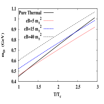
Figure 1: Variation of Debye mass with temperature

To see the competition between the temperature and the magnetic field, we have plotted the Debye mass as a function of temperature at the different strength of magnetic fields in Figure 1. At lower temperatures the magnetic field contributes more to the screening mass than the temperature whereas as the temperature increases within the SMF limit ($eB\gg T^{2}$) the thermal part plays more dominant role than the magnetic field unless the magnetic field is sufficiently strong.

Therefore the real part of retarded gluon self-energy (40) gives the real-part of the retarded resummed gluon propagator for realistic quark masses

$${\rm{Re}}D^{L}_{R}(k_{0}\rightarrow 0)=\frac{1}{\textbf{k}^{2}+m_{D}^{2}}.$$ (41)

2.2 Imaginary part of retarded gluon self-energy

Similar to the calculation of real part, the imaginary part of retarded self-energy is obtained from the real-time formalism

$$\rm{Im}~{}\Pi_{R}(k_{0},{\bf k})=\frac{\rm{Im}\bar{\Pi}(k_{0},{\bf k})}{\varepsilon(k_{0})},$$ (42)

where ${\rm{Im}}~{}\bar{\Pi}(k_{0},{\bf k})$ is derived from the off-diagonal element of self-energy matrix as

$$\rm{Im}~{}\bar{\Pi}(k_{0},{\bf k})=-\sinh(\beta k_{0}/2)\rm{Im}~{}\Pi_{12}(k_{0},{\bf k}),$$ (43)

and $\varepsilon(k_{0})$ is the theta function.

Like the evaluation of the real-part we will first evaluate the contribution due to quark-loop and then calculate for the gluon loops. Therefore the off-diagonal element (17) of the propagator matrix (15) for quarks gives the $12$-component of self-energy matrix

$$i\Pi_{12}^{L}(k) = -\frac{g^{2}}{2}\sum_{f}\int\frac{dp_{x}dp_{y}}{(2\pi)^{2}}e^{-\frac{(p+k)_{\perp}^{2}}{|q_{f}B|}}e^{-\frac{p_{\perp}^{2}}{|q_{f}B|}}$$ (44)

$$\times\int dp_{0}dp_{z}e^{\frac{\beta|p_{0}+k_{0}|}{2}}e^{\frac{\beta|p_{0}|}{2}}n_{F}(p_{0})n_{F}(p_{0}+k_{0})L^{00}\delta\left((p_{\parallel}+k_{\parallel})^{2}-m_{f}^{2}\right)\delta(p_{\parallel}^{2}-m_{f}^{2}),$$

wherein we use the equality $\sqrt{n_{F}(p_{0})(1-n_{F}(p_{0}))}=e^{\frac{\beta p_{0}}{2}}n_{F}(p_{0})$ and the trace, $L^{00}$ is evaluated as

$$L^{00} = 8\left[p_{0}(p+k)_{0}+p_{z}(p+k)_{z}+m_{f}^{2}\right].$$ (45)

The magnetic field again facilitates the calculation of the imaginary part by separating the momentum integration into components perpendicular and parallel to the magnetic field,

$${\rm{Im}}~{}\Pi_{12}^{L}(k)=\frac{g^{2}}{2}\sum_{f}{\rm{Im}}~{}\Pi_{\parallel}(k_{\parallel})~{}{\rm{Im}}~{}\Pi_{\perp}(k_{\perp}),$$ (46)

where the transverse component, $\Pi_{\perp}$ is integrated out as

$${\rm{Im}}~{}\Pi_{\perp}(k_{\perp})=\frac{|q_{f}B|}{8\pi}e^{-\frac{k_{\perp}^{2}}{2|q_{f}B|}},$$ (47)

and after performing the $p_{0}$ integration, the parallel component is given by

$${\rm{Im}}~{}\Pi_{\parallel}(k_{\parallel}) = \int\frac{dp_{z}}{2\omega_{p}}e^{\frac{\beta|\omega_{p}|}{2}}e^{\frac{\beta|k_{0}+\omega_{p}|}{2}}n(\omega_{p})n(k_{0}+\omega_{p})L^{00}(p_{0}=\omega_{p})\delta(k_{0}^{2}-k_{z}^{2}+2p_{0}\omega_{p}-2p_{z}k_{z})$$ (48)

$$+ \int\frac{dp_{z}}{2\omega_{p}}e^{\frac{\beta|\omega_{p}|}{2}}e^{\frac{\beta|k_{0}-\omega_{p}|}{2}}n(\omega_{p})n(k_{0}-\omega_{p})L^{00}(p_{0}=-\omega_{p})\delta(k_{0}^{2}-k_{z}^{2}-2k_{0}\omega_{p}-2p_{z}k_{z}).$$

Thus, in the static limit ($k_{0}\rightarrow 0$), the longitudinal component of the imaginary part of retarded self-energy (42) assumes the form

$$\lim_{k_{0}\to 0}~{}\frac{\rm{Im}\Pi_{R}^{L}(\textbf{k})}{k_{0}}=-g^{2}\sum_{f}\frac{2m_{f}^{2}}{T|k_{z}|E_{k_{z}/2}}n_{F}(E_{k_{z}/2})\left(1-n_{F}(E_{k_{z}/2})\right){\rm{Im}}~{}\Pi_{\perp}(k_{\perp}),$$ (49)

with $E_{\frac{k_{z}}{2}}=\sqrt{m^{2}_{f}+k_{z}^{2}/4}$.

In weak coupling limit, the leading-order contribution in SMF limit comes from the momentum-transferred - $|\textbf{k}|^{2}\sim\alpha_{s}eB$, thus the exponential factor in transverse component becomes unity - $\exp{(-\frac{k^{2}_{\bot}}{2\mid q_{f}B\mid})}$ $\sim$ 1. Thus the transverse component of the imaginary part of the self-energy is approximated into

$${\rm{Im}}~{}\Pi_{\perp}\approx\frac{\mid q_{f}B\mid}{8\pi}~{},$$ (50)

and the dispersion relation is simplified too:

$$E_{\frac{k_{z}}{2}}\approx\frac{\mid k_{z}\mid}{2}.$$ (51)

Furthermore using the identity

$$n_{F}(E_{\frac{k_{z}}{2}})\Big{[}1-n_{F}(E_{\frac{k_{z}}{2}})\Big{]}=\frac{1}{2\big{[}1+\cosh(\beta E_{\frac{k_{z}}{2}}\big{]}},$$ (52)

the imaginary component is rewritten as

$$\lim_{k_{0}\to 0}~{}\left[\frac{\rm{Im}~{}\Pi_{R}^{L}(\textbf{k})}{\rm k_{0}}\right]=-\frac{g^{2}}{4\pi T}\sum_{f}m^{2}_{f}\mid q_{f}B\mid\frac{1}{k_{z}^{2}\big{[}1+\cosh(\beta E_{\frac{k_{z}}{2}}\big{]}},$$ (53)

Moreover in SMF limit the longitudinal component ($\mid k_{z}\mid$) of the momentum is of the order $(\alpha_{s}eB)^{1/2}$, which is much smaller than the temperature ($<<T$). Therefore, the imaginary component of retarded self energy due to quark-loop takes further lucid form

$$\lim_{k_{0}\to 0}\Big{[}\frac{\rm{Im}\Pi^{L}_{R}(\textbf{k})}{k_{0}}\Big{]}_{\rm{quark~{}loop}}=-g^{2}\frac{\sum_{f}m^{2}_{f}\mid q_{f}B\mid}{8\pi T}\frac{1}{k^{2}_{z}}~{},$$ (54)

Similarly we will now calculate the imaginary part due to the gluon loops from the off-diagonal element of the self-energy matrix by the off-diagonal element of gluon propagator matrix (19). However, it will be easier to calculate it directly from the imaginary part of the retarded self-energy from the gluon-loop contribution (37). Thus using the identity

$$\frac{1}{x\pm{y}\pm{i\epsilon}}={\rm{P}}\left(\frac{1}{x\pm{y}}\right)\mp{i\pi{\delta(x\pm{y})}}~{},$$ (55)

the imaginary part due to the gluon-loop is extracted from (37)

$$\lim_{k_{0}\to 0}\Big{[}\frac{\rm{Im}\Pi^{L}_{R}(\textbf{k})}{k_{0}}\Big{]}_{\rm{gluon~{}loops}}=-{g^{\prime}}^{2}\frac{\pi T^{2}}{2}\frac{1}{\textbf{k}}.$$ (56)

Thus the longitudinal component of the imaginary part of gluon self-energy due to both quark and gluon-loop always factorizes into $k_{0}$ times $\rm{Im}\Pi^{L}_{R}(\bf k)$ so it vanishes in the static limit ($k_{0}\to 0$). Therefore, using the factors in (6, 7), the resummed symmetric propagator (5) in the static limit reduces to

$$D^{L}_{S}(\textbf{k}) = [1+2n_{B}(k_{0})]~{}{\rm{sgn}}(k_{0})\left(D^{L}_{R}(k)-D^{L}_{A}(k)\right)$$ (57)

$$= i4T\frac{{\rm{Im}}\Pi^{L}_{R}(\textbf{k})}{\left[\textbf{k}^{2}-\rm{Re}\Pi^{L}_{R}(\textbf{k})\right]^{2}},$$

which is however decomposed into the contributions due to the quark and gluon loop

$$D^{L}_{S}(\textbf{k}) = D^{L}_{S}(\textbf{k})_{\rm{quark~{}loop}}+D^{L}_{S}(\textbf{k})_{\rm{gluon~{}loop}}$$ (58)

with

$$D^{L}_{S}(\textbf{k})_{\rm{quark~{}loop}} = -\frac{ig^{2}}{2\pi k^{2}_{z}}\frac{\sum_{f}\mid q_{f}B\mid m^{2}_{f}}{({\textbf{k}}^{2}+m^{2}_{D})^{2}}$$ (59)

$$D^{L}_{S}(\textbf{k})_{\rm{gluon~{}loop}} = \frac{-2i\pi{g^{\prime}}^{2}T^{3}}{\textbf{k}({\textbf{k}}^{2}+m_{D}^{2})^{2}}~{}.$$ (60)

3 Heavy quark potential

The derivation of potential between a heavy quark $Q$ and its anti-quark ($\bar{Q}$) from effective field theory, namely pNRQCD may not be plausible because the hierarchy of non relativistic scales and thermal scales assumed in weak coupling EFT calculations may not be satisfied. Even in the first principle QCD study, the adequate quality of the data is not available in the present lattice correlator studies so one may use the potential model to circumvent the problems. Since the mass of the heavy quark ($m_{Q}$) is very large, so the requirement - $m_{Q}\gg T\gg\Lambda_{QCD}$ is satisfied for the description of the interactions between a pair of heavy quark and anti-quark at finite temperature in strong magnetic field limit in terms of quantum mechanical potential. Thus we can obtain the medium-modification to the vacuum potential in the presence of magnetic field by correcting both its short and long-distance part with a dielectric function $\epsilon(\textbf{k})$ as

$$V(r;T,B)=\int\frac{d^{3}\textbf{k}}{(2\pi)^{3/2}}({e^{i\textbf{k}.\textbf{r}}-1})\frac{V(\textbf{k})}{\epsilon(\textbf{k})},$$ (61)

where we have subtracted a $r$-independent term to renormalize the heavy quark free energy, which is the perturbative free energy of quarkonium at infinite separation. The Fourier transform, $V(\textbf{k})$ of the Cornell potential is given by

$${V}(\textbf{k})=-\frac{4}{3}\sqrt{\frac{2}{\pi}}\frac{\alpha_{s}}{\textbf{k}^{2}}-\frac{4\sigma}{\sqrt{2\pi}\textbf{k}^{4}},$$ (62)

and the dielectric permittivity, $\epsilon(\mathbf{k})$ encodes the effects of deconfined medium in the presence of magnetic field, which is going to be calculated next.

3.1 The complex permittivity for a hot QCD medium in a strong magnetic field

The dielectric permittivity is defined by the static limit of 11-component of longitudinal resummed gluon propagator by the following equation

$$\frac{1}{\epsilon(\bf{k})}=\displaystyle{\lim_{k_{0}\rightarrow 0}}{\textbf{k}}^{2}D_{11}^{L}(k_{0},\textbf{k}),$$ (63)

where the real and imaginary parts of $D^{L}_{11}(\textbf{k})$ are obtained by the retarded (or advanced) and symmetric propagator, respectively

$$\rm{Re}D^{L}_{11}(\textbf{k}) = \rm{Re}D^{L}_{R}(\textbf{k})$$

$$\rm{Im}D^{L}_{11}(\textbf{k}) = \rm{Im}\frac{D^{L}_{S}}{2}(\textbf{k}),$$ (64)

which will in turn gives the real and imaginary part of dielectric permittivity, respectively.

Thus the static limit of resummed retarded propagator (41) gives the real part of dielectric permittivity

$$\frac{1}{{\rm Re}~{}\epsilon(\bf{k})}=\frac{\textbf{k}^{2}}{\textbf{k}^{2}+m_{D}^{2}}.$$ (65)

Similarly the static limit of resummed symmetric propagators (59, 60) gives the imaginary part of dielectric permittivity, due to quark and gluon loop contributions

$$\frac{1}{\rm{Im}~{}{\epsilon(\bf{k})}_{\rm quark~{}loop}} = -\frac{g^{2}}{4\pi}\sum_{f}m_{f}^{2}\mid q_{f}B\mid\frac{{\bf k}^{2}}{k^{2}_{z}({\bf{k}}^{2}+m_{D}^{2})^{2}}~{},$$ (66)

$$\frac{1}{{{\rm{Im}}~{}\epsilon(\bf k)}_{\rm gluon~{}loop}} = -{g^{\prime}}^{2}\pi T^{3}\frac{{\bf{k}}^{2}}{\bf{k}({{\bf{k}}^{2}+m_{D}^{2})}^{2}}~{},$$ (67)

respectively.

Therefore the real and imaginary part of dielectric permittivities give the real and imaginary part of the complex potential, respectively in the next subsection.

3.2 Real and Imaginary Part of the potential

The real-part of dielectric permittivity (65) is substituted into the definition (61) to give the real part of $Q\bar{Q}$ potential in the presence of strong magnetic field [17] (with $\hat{r}=rm_{D}$)

$$\rm{Re}V(r;T,B) = -\frac{4}{3}\alpha_{s}m_{D}\frac{e^{-\hat{r}}}{\hat{r}}+\frac{2\sigma}{m_{D}}\frac{(e^{-\hat{r}}-1)}{\hat{r}}$$ (68)

$$- \frac{4}{3}\alpha_{s}m_{D}+\frac{2\sigma}{m_{D}}~{},$$

where the dependence of temperature and magnetic field enter through the Debye mass. The nonlocal terms insure the potential in medium $V(r;T,B)$ to reduce to the potential in $(T,B)\rightarrow 0$ limit, which are, however, required to compute the masses of quarkonium states. The additional effect due to the strong magnetic field on the potential in a hot QCD medium is displayed as a function of interparticle distance ($r$) for different strength of magnetic fields in Figure 2, after excluding the constant terms from (68). The solid line represents the potential in a pure thermal medium (i.e. in the absence of magnetic field) whereas the dashed and dotted lines denote the effect of strong magnetic fields, 10 and 25 $m_{\pi}^{2}$ to a thermal medium, respectively. We have found that the magnetic field (eB=10 $m_{\pi}^{2}$) affects the linear string term more than the Coulomb term, as a result, the overall potential at small and intermediate $r$ becomes less screened than the potential in pure thermal medium. However, further increase of magnetic field (i.e. eB= 25 $m_{\pi}^{2}$), the potential becomes less attractive than eB=10 $m_{\pi}^{2}$. However for large $r$ the effect of magnetic field diminishes gradually.

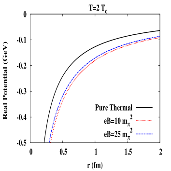
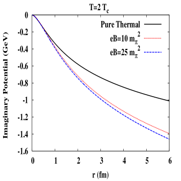
Figure 2: Real (left) and imaginary (right) part of the potential

Similarly the imaginary part of the potential is obtained by plugging the imaginary part of dielectric permittivities due to quark-loop (66) and gluon-loop (67) contributions into the definition of potential (61). The imaginary component of the potential consists of Coulomb and string terms

$$\rm{Im}~{}V(r;T,B)=\rm{Im}~{}V_{C}(r;T,B)+\rm{Im}~{}V_{S}(r;T,B),$$ (69)

where each term is again split into quark-loop ($q$) and gluon-loop ($g$) contributions. We will first calculate due to the quark loop from (66)

$$\rm{Im}V_{C}^{q}(r;T,B) = \int\frac{d^{3}\textbf{k}}{(2\pi)^{3/2}}\left(e^{ik.r}-1\right)\left(-\frac{4}{3}\sqrt{\frac{2}{\pi}}\frac{\alpha_{s}}{{\textbf{k}}^{2}}\right)\left(-\frac{g^{2}{\textbf{k}}^{2}}{4\pi k^{2}_{z}}\frac{\sum_{f}\mid q_{f}B\mid m^{2}_{f}}{{({\textbf{k}}^{2}+m^{2}_{D})}^{2}}\right)$$ (70)

$$= \frac{\alpha_{s}g^{2}}{3\pi^{2}}\left(\sum_{f}\mid q_{f}B\mid m^{2}_{f}\right)I_{C},$$

where the momentum integral, $I_{C}$ is integrated as

$$I_{C} = \int_{0}^{\infty}\frac{dk}{{({\textbf{k}}^{2}+m^{2}_{D})}^{2}}\int_{-1}^{1}dx\frac{(e^{ikrx}-1)}{x^{2}}$$ (71)

$$= \int_{0}^{\infty}\frac{dk}{{({\textbf{k}}^{2}+m^{2}_{D})}^{2}}\left[2-2\cos(kr)-2kr~{}Si(kr)\right]$$

$$\equiv I_{C1}+I_{C2}+I_{C3},$$

where

$$I_{C1} = 2\int_{0}^{\infty}\frac{dk}{{({\textbf{k}}^{2}+m^{2}_{D})}^{2}}=\frac{\pi}{2m_{D}^{3}}$$ (72)

$$I_{C2} = -2\int_{0}^{\infty}\frac{\cos kr~{}dk}{{({\textbf{k}}^{2}+m^{2}_{D})}^{2}}=-\left[\frac{\pi e^{-\hat{r}}}{2m_{D}^{3}}+\frac{\hat{r}\pi e^{-\hat{r}}}{2m_{D}^{3}}\right]$$ (73)

$$I_{C3} = -2r\int_{0}^{\infty}\frac{dk~{}k}{{({\textbf{k}}^{2}+m^{2}_{D})}^{2}}Si(kr)$$ (74)

$$= -2\frac{\hat{r}}{m_{D}}\int_{0}^{\infty}\frac{dk~{}k}{{({\textbf{k}}^{2}+m^{2}_{D})}^{2}}\int_{0}^{kr}dx\frac{\sin x}{x}~{},$$

respectively. Similarly the string part of the imaginary potential is

$$\rm{Im}V_{S}^{q}(r;T,B) = \int\frac{d^{3}\textbf{k}}{(2\pi)^{3/2}}\left(e^{ik.r}-1\right)\left(-\frac{4\sigma}{\sqrt{2\pi}{\textbf{k}}^{4}}\right)\left(-\frac{g^{2}{\textbf{k}}^{2}}{4\pi k^{2}_{z}}\frac{\sum_{f}\mid q_{f}B\mid m^{2}_{f}}{{({\textbf{k}}^{2}+m^{2}_{D})}^{2}}\right)$$ (75)

$$= \frac{\sigma g^{2}}{2\pi^{2}}\left(\sum_{f}\mid q_{f}B\mid m^{2}_{f}\right)I_{S},$$

where the integral, $I_{S}$ is evaluated as

$$I_{S} = \int_{0}^{\infty}\frac{dk}{{\textbf{k}}^{2}{({\textbf{k}}^{2}+m^{2}_{D})}^{2}}\int_{-1}^{1}dx\frac{(e^{ikrx}-1)}{x^{2}}$$ (76)

$$= \int_{0}^{\infty}\frac{dk}{{\textbf{k}}^{2}{({\textbf{k}}^{2}+m^{2}_{D})}^{2}}\left[2-2\cos(kr)-2krSi(kr)\right]$$

$$\equiv I_{S1}+I_{S2},$$

where $I_{S1}$ and $I_{S2}$ are given by

$$I_{S1} = \int_{0}^{\infty}\frac{dk}{{\textbf{k}^{2}{({\textbf{k}}^{2}+m^{2}_{D})}^{2}}}\left(2-2cos(kr)\right)$$ (77)

$$= \frac{\pi}{2m_{D}^{5}}\left[\hat{r}e^{-\hat{r}}-3(1-e^{-\hat{r}})+2\hat{r}\right]$$

$$I_{S2} = -2\frac{\hat{r}}{m_{D}}\int_{0}^{\infty}\frac{dk}{{{k}{({\textbf{k}}^{2}+m^{2}_{D})}^{2}}}\int_{0}^{kr}\frac{\sin x}{x}dx,$$ (78)

Next we calculate the imaginary part due to the gluon loop contribution (67) for the Coulomb and string terms, respectively [12] as

$$\rm{Im}V^{g}_{C}(r;T,B) = -\frac{8{\alpha_{s}}^{\prime}T}{3}\int_{0}^{\infty}\frac{dz~{}z}{(z^{2}+1)^{2}}\left(1-\frac{\sin{z\hat{r}}}{z\hat{r}}\right)$$ (79)

$$\rm{Im}V_{S}^{g}(r;T,B) = -\frac{4\sigma T}{m_{D}^{2}}\int_{0}^{\infty}\frac{dz}{z(z^{2}+1)^{2}}\left(1-\frac{\sin{z\hat{r}}}{z\hat{r}}\right)~{},$$ (80)

where the Debye mass is given by Eq.(40).

Thus the equations (70) and (79) give the Coulombic contribution whereas the equations (75), (80) give the string contribution

$${\rm{Im}}~{}V_{C}(r;T,B) = \rm{Im}V^{q}_{C}(r;T,B)+\rm{Im}V^{g}_{C}(r;T,B)$$ (81)

$${\rm{Im}}~{}V_{S}(r;T,B) = \rm{Im}V^{q}_{S}(r;T,B)+\rm{Im}V^{g}_{S}(r;T,B)$$ (82)

to the imaginary component of the potential, respectively. Like the real-part of potential, how does the imaginary part get affected by the additional presence of magnetic field we have plotted it as a function of interquark distance in the right panel of Figure 2. In pure thermal medium (denoted by solid line), both Coulomb and string term are larger powers of $\hat{r}$ and counter each other, resulting the overall magnitude very small. Now the strong magnetic field not only reduces the power of $\hat{r}$ in both terms compared to the pure thermal medium, it induces Coulomb and string terms to contribute additively, resulting the overall magnitude of imaginary part larger. The above observation ultimately translates into the enhancement of thermal width of resonance states due to the ambient strong magnetic field.

4 Properties of Quarkonia

4.1 Wavefunction and Binding Energy

To investigate the properties of quarkonia in a strong magnetic field, we first solve the Schrödinger equation numerically by employing the real part of the potential (68) to see how the eigenstates to $J/\psi$, $\psi^{\prime}$ and $\chi_{c}$ states in a thermal QCD medium get affected by the presence of strong magnetic field in figures 3-5, respectively. In the presence of magnetic field both wavefunction and probability distribution of quarkonia becomes sharply peaked compared to quarkonia in absence of magnetic field.

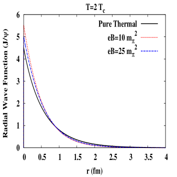
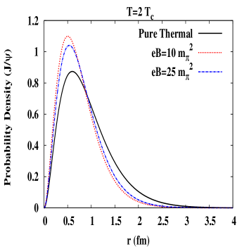
Figure 3: The wavefunction and the radial probability density of $J/\psi$ state

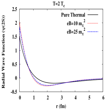
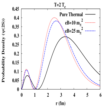
Figure 4: The wavefunction and the radial probability density of $\psi^{\prime}$ state

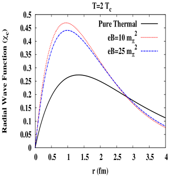
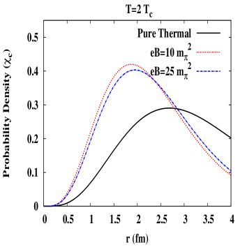
Figure 5: The wavefunction and the radial probability density of $\chi_{c}$ state

Thus the medium effects encoded into the wavefunctions ($\Phi(r)$) and the corresponding probability distributions explore how the average size of a particular quarkonia ($\sqrt{{r_{i}}^{2}}$ =${(\int d\tau~{}r^{2}~{}{\mid\Phi_{i}(r)\mid}^{2})}^{1/2}$) get affected due to a thermal medium in absence (presence) of magnetic field in left (right) panel of Figure 6, respectively. The magnetic field in general causes swelling of all resonances unless the temperature is very large (Figure 7).

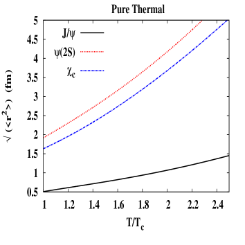
Figure 6: The average size ($\sqrt{r^{2}}$) of quarkonia in pure thermal medium (left) and then thermal medium in presence of strong magnetic field (right)

Figure 7: Variation of the size of quarkonia with the magnetic field at a fixed temperature.

Finally we have studied how the binding energies of quarkonia change with the temperature in absence (presence) of magnetic field in left (right) panel of Figure 8, respectively. The immediate observation is that the magnetic field causes the binding energy to decrease with the temperature slowly, compared to the medium in absence of magnetic field. Moreover the competition between the scales associated to the temperature and magnetic field affects the binding of quarkonia discriminately, viz. $J/\psi$ becomes less bound and $\chi_{c}$ becomes more bound due to the presence of magnetic field. However, the binding energy decreases with the magnetic field too (Figure 9).

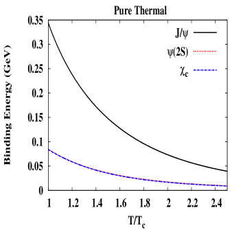
Figure 8: The binding energies of quarkonia in pure thermal medium (left) and thermal medium in presence of magnetic field (right).

Figure 9: Variation of binding energies with the magnetic field

4.2 Thermal Width and Dissociation of Quarkonia

Using the first-order perturbation theory, the width ($\Gamma$) has been evaluated numerically by folding the eigenstates of a specific quarkonium state in the deconfined medium in the presence of magnetic field

$$\Gamma=-2\int_{0}^{\infty}\rm{Im}~{}V(r;B,T)|\Phi_{i}(r)|^{2}d\tau.$$ (83)

We have thus computed the width as a function of temperature in absence (presence) of magnetic field in the left (right) panel of Figure 10, respectively. We have found that in pure thermal medium (left panel) the width increases with the temperature faster than in the presence of strong magnetic field (right panel). However, the magnetic field always enhances the width of the resonances (Figure 11).

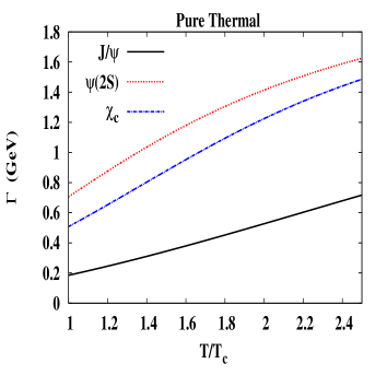
Figure 10: Variation of the thermal widths with the temperature of the medium in absence (left) as well as presence (right) of magnetic field

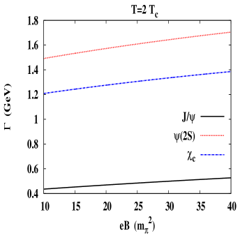
Figure 11: Thermal widths of quarkonia is plotted as a function of magnetic field

Having studied the change of properties of quarkonia in the presence of magnetic field, we investigate now the effect of strong magnetic field on the dissociation of quarkonia from the conservative criterion on the width of the resonance in $\Gamma\geq 2\rm{Re}~{}{\rm{B.E.}}$ [29]. So we have first estimated the dissociation temperatures of quarkonia in absence of magnetic field in the Table 1 and then did the same in presence of magnetic fields in Table 2. We found that the dissociation temperatures increase due to the presence of strong magnetic field but with the further increase of magnetic field the dissociation temperatures decrease. For example, $J/\psi$’s and $\chi_{c}$’s are dissociated at higher temperatures at 2 $T_{c}$ and 1.1 $T_{c}$ at a magnetic field $eB\approx 6~{}{\rm{and}}~{}4~{}m_{\pi}^{2}$, respectively, compared to the values 1.60 $T_{c}$ and 0.80$T_{c}$ in the absence of magnetic field, respectively. However, the $J/\psi$ is dissociated at smaller temperatures, 1.8 $T_{c}$ and 1.5 $T_{c}$ for higher magnetic fields, $eB=27~{}{\rm{and}}~{}68~{}m_{\pi}^{2}$, respectively. Similarly for higher magnetic field, $eB=12~{}m_{\pi}^{2}$, $\chi_{c}$ gets dissociated at the critical temperature.

State	Dissociation Temperature
	$T_{D}$ (in $T_{c}$)
$J/\psi$	1.60
$\chi_{c}$	0.80
$\psi(2S)$	0.70

Table 1: Dissociation temperature for thermal medium in absence of magnetic field

State	Dissociation Temperature (Magnetic field)
	$T_{D}/T_{c}$ ($eB$ ($m^{2}_{\pi}$))
$J/\psi$	2.0 (6.50)
	1.8 (27.0)
	1.5 (68.0)
$\chi_{c}$	1.1 (3.7)
	1.0 (12)
$\psi(2S)$	$<1(<m^{2}_{\pi}$)

Table 2: Dissociation temperature for thermal medium in presence of magnetic field

5 Conclusion

The noncentral events in ultra-relativistic heavy-ion collisions provide an opportunity to probe the properties of heavy quarkonia in the presence of a strong magnetic field. So we utilize this by calculating the bound state radii, binding energy, thermal width etc. of quarkonia by resummed perturbative thermal QCD in the presence of strong magnetic field, thereby studying the dissociation of quarkonia due to the Landau damping. For that purpose, using the Keldysh representation in real-time formalism, we have first calculated the real and imaginary parts of retarded gluon self-energy for a deconfined medium in a strong magnetic field by thermalizing the Schwinger proper-time fermion propagator and then calculate the resummed retarded and symmetric propagators by the Schwinger-Dyson equation. As a result, the Fourier components of both short and long distance components of $Q\bar{Q}$ interaction are being modified by the static limit of resummed propagators and its inverse Fourier transform gives rise the real and imaginary part of potential in coordinate space. We have noticed that the long-distance term is largely affected by the magnetic field than the shot-distance term, as a result the real part of potential becomes stronger and the imaginary part becomes larger than the medium in absence of magnetic field.

We have then studied the quarkonium dissociation by investigating its properties by solving the Schrodinger equation numerically with potential derived to check how the states and the probability distributions of quarkonia change in the strong magnetic field. With the solutions of Schrödinger equation we have then calculated the average size, binding energy, thermal width of resonances. We have found that the presence of strong magnetic field causes the swelling for $J/\psi$ and squeezing for $\chi_{c}$. Similarly the binding decreases for $J/\psi$ and increases for $\chi_{c}$. Moreover the binding energies decrease with the temperature of medium very slowly due to the presence of magnetic field and for a given medium the binding decreases with the increase in magnetic fields. On the other hand the presence of magnetic field causes an increase the width of resonances in a hot QCD medium.

The above observations on the change of the properties of quarkonia in a strong magnetic field facilitate to study the dissociation of quarkonia due to the Landau damping and quantify the magnetic field at which a specific $Q\bar{Q}$ state excites to the continuum from the intersection of the magnetic field induced thermal width and the (twice) binding energy curve. We have noticed that the presence of strong magnetic field increase the dissociation temperatures but it decreases with the further increase of magnetic field. For example, $J/\psi$’s and $\chi_{c}$’s are dissociated at higher temperatures at 2 $T_{c}$ and 1.1 $T_{c}$ at a magnetic field $eB\approx 6m_{\pi}^{2}$ and $4m_{\pi}^{2}$, respectively, compared to the values 1.60 $T_{c}$ and 0.8 $T_{c}$ in the absence of magnetic field, respectively.

6 Acknowledgement

BKP is thankful to the CSIR (Grant No.03 (1407)/17/EMR-II), Government of India for the financial assistance.

References

• [1] V. Skokov, A. Illarionov, and V. Toneev, Int. J. Mod. Phys. A 24, 5925 (2009).
• [2] V. Voronyuk, V. D. Toneev, W. Cassing, E. L. Bratkovskaya, V. P. Konchakovski, S .A. Voloshin, Phys. Rev. C 83, 054911 (2011).
• [3] T. Vachaspati, Phys.Lett. B 265 258-261 (1991).
• [4] K. Tuchin, Phys. Rev. C 82, 034904 (2010).
• [5] W. M. Alberico, A. Beraudo, A. De Pace, A. Molinari, Phys. Rev. D 77, 017502 (2008).
• [6] T. Matsui and H. Satz, Phys. Lett. B 178, 416 (1986).
• [7] M. A. Escobedo and J. Soto, Phys. Rev. A 78, 032520 (2008).
• [8] N. Brambilla, J. Ghiglieri, A. Vairo and P. Petreczky, Phys. Rev. D 78, 014017 (2008).
• [9] M. Laine, O. Philipsen, P. Romatschke, and M. Tassler,  JHEP 0703, 054 (2007).
• [10] A. Beraudo, J. P. Blaizot, C. Ratti, Nucl. Phys. A 806, 312 (2008).
• [11] N. Brambilla, M. A. Escobedo, J. Ghiglieri, and A. Vairo, JHEP 1305, 130 (2013).
• [12] Lata Thakur, Uttam Kakade and Binoy Krishna Patra, Phys. Rev. D 89, 094020 (2014).
• [13] Adrian Dumitru, Yun Guo, Michael Strickland, Phys. Rev. D79, 114003 (2009).
• [14] B. K. Patra, H. Khanchandani, and L. Thakur, Phys Rev D 92, 085034 (2015).
• [15] B. K. Patra, H. Khanchandani,
• [16] A. Rothkopf, T. Hatsuda and S. Sasaki, Phys. Rev. Lett.  108, 162001 (2012).
• [17] Mujeeb Hasan, Bhaswar Chatterjee and Binoy Krishna Patra, Eur. Phys. J. C 77, 767 (2017).
• [18] Shubhalaxmi Rath, Binoy Krishna Patra, JHEP 1712, 098 (2017).
• [19] Balbeer Singh, Lata Thakur, Hiranmaya Mishra. arXiv:1711.03071 [hep-ph].
• [20] Magaret E. Carrington, H. Defu, Markus H. Thoma, Eur. Phys. J. C 7, 347-354 (1999).
• [21] J. Schwinger, Phys. Rev. 82, 664 (1951).
• [22] Wu-yang Tsai, Phys. Rev. D 10, 2699 (1974).
• [23] T. Chyi et. al, Phys. Rev. D 62, 105014 (2000).
• [24] K. Fukushima, K. Hattori, H-U. Yee and Y. Yin, Phys. Rev. D 93, 074028 (2016).
• [25] A. Bandyopadhyay, C. A. Islam and M. G. Mustafa, Phys. Rev. D 94, 114034 (2016).
• [26] E. J. Ferrer, V. de la Incera and X. J. Wen, Phys. Rev. D 91, 054006 (2015).
• [27] Yu. A. Simonov, Phys. At. Nucl. 58, 107 (1995).
• [28] M. A. Andreichikov, V. D. Orlovsky and Yu. A. Simonov, Phys. Rev. Lett. 110, 162002 (2013).
• [29] A. Mocsy and P. Petreczky, Phys. Rev. Lett. 99, 211602 (2007).