The selection function of the LAMOST Spectroscopic Survey of the Galactic Anticentre

Abstract

We present a detailed analysis of the selection function of the LAMOST Spectroscopic Survey of the Galactic Anti-centre (LSS-GAC). LSS-GAC was designed to obtain low resolution optical spectra for a sample of more than 3 million stars in the Galactic anti-centre. The second release of value-added catalogues of the LSS-GAC (LSS-GAC DR2) contains stellar parameters, including radial velocity, atmospheric parameters, elemental abundances and absolute magnitudes deduced from 1.8 million spectra of 1.4 million unique stars targeted by the LSS-GAC between 2011 and 2014. For many studies using this database, such as those investigating the chemodynamical structure of the Milky Way, a detailed understanding of the selection function of the survey is indispensable. In this paper, we describe how the selection function of the LSS-GAC can be evaluated to sufficient detail and provide selection function corrections for all spectroscopic measurements with reliable parameters released in LSS-GAC DR2. The results, to be released as new entries in the LSS-GAC value-added catalogues, can be used to correct the selection effects of the catalogue for scientific studies of various purposes.

1 Introduction

Large-scale spectroscopic surveys of Galactic stars, e.g. the Sloan Extension for Galactic Understanding and Exploration (SEGUE; Yanny et al. 2009) and the LAMOST Experiment for Galactic Understanding and Exploration (LEGUE; Deng et al. 2012; Zhao et al. 2012), are opening a new window for the study of the formation and evolution of the Milky Way galaxy in great detail. However, unlike photometric surveys that yield, in general, complete samples of objects to a given limiting magnitude, time-consuming spectroscopic surveys often have to select targets, and are unavoidably affected by the various potential target selection effects. Bias arises from the target selection, the observation, data reduction and processes determining parameters. To understand the relationship between a spectroscopic sample of stars with a reliable estimation of parameters and the parent stellar population, one needs to study and account for the selection function.

Many authors have made efforts to characterise the selection function of spectroscopic samples from various completed or on-going surveys. Cheng et al. (2012) determine the selection function of a sample of SEGUE main-sequence turn-off stars. Schlesinger et al. (2012) study and correct for the various selection biases of SEGUE G and K dwarfs. Selection effects are also considered in Bovy et al. (2012) and Liu & van de Ven (2012) for SEGUE G dwarfs for different purposes. Nidever et al. (2014) characterise the selection effects of the Apache Point Observatory Galactic Evolution Experiment (APOGEE; Majewski et al. 2015) red clump stars. More recently, Stonkutė et al. (2016) discuss the selection function of Milky Way field stars targeted by the Gaia-ESO survey (Gilmore et al., 2012), and Wojno et al. (2017) describe in detail the selection function of the Radial Velocity Experiment (RAVE; Steinmetz et al. 2006) survey.

In this paper, we take efforts to analyze the selection function of the LAMOST spectroscopic Survey of the Galactic Anticentre (LSS-GAC; Liu et al. 2014, 2015; Yuan et al. 2015). LSS-GAC is a major component of LEGUE. It was initiated in October, 2012, following a year-long Pilot Survey. It aims to observe $\sim$ 3 million stars of all colours and magnitudes of $r$ $\lesssim$17.8 mag (18.5 for a limited number of fields) in a large (3,400 deg²) and continuous sky area centred on the Galactic anti-centre (GAC). The survey should allow us to obtain a deeper understanding of the structure, formation and evolution of the Milky Way disk(s), and of the Galaxy as a whole.

Data yielded by the LSS-GAC survey are available from the LAMOST official data releases, such as LAMOST DR1 (Luo et al., 2015). The official data releases include stellar spectra and stellar parameters derived with the LAMOST Stellar parameter Pipeline (LASP; Wu et al. 2011, 2014). In addition, there are public releases of LSS-GAC value-added catalogues, the LSS-GAC DR1 (Yuan et al., 2015) and LSS-GAC DR2 (Xiang et al., 2017a). The LSS-GAC DR1 contains radial velocities and stellar atmospheric parameters derived with a different stellar parameter pipeline, the LAMOST Stellar Parameter Pipeline at Peking University (LSP3; Xiang et al. 2015a), for LAMOST spectroscopic observations between September, 2011 and June, 2013. The catalogue also presents additional information, including multiband photometry and proper motions collected from various databases, as well as extinction, distance and orbital parameters deduced with a variety of techniques. For LSS-GAC DR2, in addition to the above information, $\alpha$-element abundances, C and N abundances, and absolute magnitudes derived from the improved LSP3 (Xiang et al., 2017b) are also provided for LAMOST spectroscopic observations between September, 2011 and June, 2014.

In this paper we present a detailed study of the selection function of LSS-GAC based on its most recent data release, LSS-GAC DR2 (Xiang et al., 2017a), to facilitate broad and robust usage of this publicly-available database. There have already been several studies trying to characterise the selection function of stars targeted by LSS-GAC. Rebassa-Mansergas et al. (2015) have discussed the selection function of a small sample of white dwarfs identified in an early stage of LSS-GAC in a study aimed to determine the mass function of Galactic white dwarfs. Xiang et al. (2015b) have carried out a detailed analysis of the selection effects of LSS-GAC F-type turn off stars that they used to determine metallicity gradients of the Milky Way disk. Liu et al. (2017) take the selection effects of LAMOST K giants into account when deriving the stellar number density distribution.

However, a comprehensive analysis of the selection function of LSS-GAC is still lacking. The earlier efforts of Rebassa-Mansergas et al. (2015), Xiang et al. (2015b), and Liu et al. (2017) all concentrate on specific samples selected from LSS-GAC. In addition, Liu et al. (2017) determine the selection function of stars on the basis of the individual LAMOST plates, which have a field of view (FoV) of $\sim$20 deg². The approach is not suitable for LSS-GAC, which selects targets based on boxes of $\sim$ 1 deg² in sky area. Given the steep stellar number density gradients with latitude near the Galactic plane, the selection function in different parts of a given LAMOST plate near the plane would be quite different. Furthermore, LAMOST is equipped with 16 spectrographs that have different throughputs, decreasing in general with distance from the field centre (Yuan et al., 2015). Clearly, such variations of the selection function can not be ignored. Xiang et al. (2015b) improve the work by determining the selection function spectrograph by spectrograph. However in evaluating the selection function, they have combined stars in a given spectrograph targeted by all LAMOST plates that share the same central star. Different plates are usually observed under different weather conditions including transparency, seeing and lunar phase, and are thus likely to have different limiting magnitudes. The selection function is expected to differ significantly amongst different plates. Furthermore, in some rare cases, although two plates target the same field, the sky areas targeted by the individual spectrographs of the two plates actually differ. Thus evaluating the selection function by combining data from the different plates is inappropriate.

In this work, we discuss in detail the selection function of spectroscopic measurements of stars catalogued in the LSS-GAC DR2 and give a robust way to evaluate the selection bias, by considering as many effects as possible. Mock data are used to test our technique for the selection function evaluation. The paper is organised as follows. In §2 we introduce briefly the LSS-GAC, including the target selection algorithm and the LSS-GAC DR2. In §3 we describe how we evaluate the selection function of LSS-GAC. In §4 we test our algorithm using mock data. We discuss the applications of our results in §5 and summarise in §6.

2 LSS-GAC

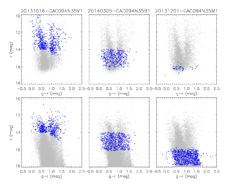
Figure 1: Target selection for three LSS-GAC example plates all centred on RA = 94.39059°and Dec = 35.14920°. The grey dots represent all stars in the clean photometric samples of the field. The blue dots represent all those selected and observed objects by the three LSS-GAC plates. The upper and bottom rows are based on the APASS DR9 and XSTPS-GAC photometric catalogues, respectively. The left, middle and right columns show target selection for the VB, B and M plates, respectively. The observational dates and IDs of the individual plates are labeled at the top of the three columns.

LSS-GAC contains three different components, the main, the M31/M33 and the VB surveys. The main survey aims to observe about 3 million stars in a contiguous sky area towards the GAC (150°$<l<$ 210°, and $-$30°$<b<$30°). The M31/M33 survey observes all kinds of interesting targets in the vicinity fields of M31 and M33 within the reach of LAMOST, including supergiants, massive star clusters, planetary nebulae, $\rm H~{}{\scriptstyle II}$ regions, as well as background QSOs, galaxies and foreground Galactic stars. The VB survey is designed to observe very bright (VB) stars (9 $<r<$ 14 mag) in sky areas accessible to LAMOST ($-$10$\degr<{\rm Dec}<$ 60°) for time of non-ideal observing conditions such as in bright/grey lunar nights.

In this section we will give a brief introduction to the LSS-GAC survey and its most recent data release, LSS-GAC DR2. Liu et al. (2014) introduce the survey design and scientific motivations of LSS-GAC. Yuan et al. (2015) present the target selection and the LSS-GAC DR1. Liu et al. (2015) give a review of the early scientific results. Xiang et al. (2015a, c) and Xiang et al. (2017b) describe the data reduction of LSS-GAC and Xiang et al. (2017a) present the LSS-GAC DR2.

2.1 Target selection

Four different types of survey plates, namely, very bright (VB) , bright (B), median bright (M) and faint (F) plates, are designed for LSS-GAC. They are defined by different $r$-band magnitude ranges. Usually, VB plates target stars of $r<14$ mag. B, M and F plates target stars of $14<r\leq m_{1}$ mag, $m_{1}<r\leq m_{2}$ mag and $m_{2}\leq r<18.5$ mag, respectively. Here $m_{1}$ and $m_{2}$ are the border magnitudes separating B, M and F plates and differ slightly for different regions in the sky (Yuan et al., 2015). Typical values of $m_{1}$ and $m_{2}$ are 16.3 and 17.8 mag, respectively. Except for some VB plates, LSS-GAC targets are selected from the photometric catalogues of Xuyi Schmidt Telescope Photometric Survey of the Galactic Anticentre (XSTPS-GAC; Liu et al. 2014; Yuan et al. 2015).

XSTPS-GAC surveys an area of approximately 7,000 deg² in the GAC area, including the M31/M33 region, using the Xuyi 1.04/1.20m Schmidt Telescope. It collects images in SDSS $g$, $r$ and $i$ bands. XSTPS-GAC catalogues about one hundred million stars down to a limiting magnitude of $r$ $\sim$ 19.0 mag (10$\sigma$). The photometric systematic uncertainties of XSTPS-GAC are estimated to be smaller than 0.02 mag (Yuan et al., in preparation), and the uncertainties of resulted RA and Dec are about 0.1 arcsec (Zhang et al., 2014).

The basic strategy of the LSS-GAC target selection is to uniformly and randomly select stars from the colour-magnitude diagrams (Yuan et al., 2015). A brief summary of the target selection procedure for the LSS-GAC B, M and F plates is as follows:

1. The XSTPS-GAC photometric catalogue is used to generate a clean sample of targets for LSS-GAC, excluding stars that are either poorly detected, badly positioned, flagged as galaxies or star pairs, or contaminated by bright neighbours or by sky background.

2. The whole survey area is divided into boxes of 1 deg side in RA and Dec. For stars in each box, ($r$, $g-r$) and ($r,$ $r-i$) Hess diagrams are constructed from the clean sample. Stars of extremely blue colours, $(g-r)$ or $(r-i)$ $<-$0.5 mag, and of extremely red colours, $(g-r)$ or $(r-i)$ $>$ 2.5 mag, are first selected.

3. Stars in the remaining colour space are then sorted in magnitude from bright to faint. $m_{1}$ and $m_{2}$ are set to the faint end magnitudes of the first 40% and 80% sources, respectively.

4. Stars of B, M and F plates are selected and assigned priorities, in batches of 200 stars per deg², with a Monte Carlo (random) approach.

5. The field centres of the individual LAMOST plates are defined. All LAMOST plates must be centred on bright stars ($\lesssim 8$ mag) such that the LAMOST active optics can operate.

6. For each plate, the SSS software (Luo et al., 2015) is used to allocate fibres to the selected stars.

The target selection of VB plates is slightly different from B, M and F plates. Within the XSTPS-GAC footprint, all stars of $r\leq$ 14.0 mag from XSTPS-GAC and all stars of 9 $\leq J\leq$ 12.5 mag from Two Micron All-Sky Survey (2MASS; Skrutskie et al. 2006) are selected as potential targets with equal priorities. Outside the XSTPS-GAC footprint, all stars of 10.0 $\leq b1\leq$ 15.0 mag, or 10.0 $\leq b2\leq$ 15.0 mag, or 9.0 $\leq r1\leq$ 14.0 mag, or 9.0 $\leq r2\leq$ 14.0 mag, or 8.5 $\leq i\leq$ 13.5mag from PPMXL (Roeser et al., 2010) and stars of 9 $\leq J\leq$ 12.5 mag from 2MASS are selected as potential targets with equal priorities.

2.2 Observation, data reduction and the LSS-GAC DR2

The five-year long Phase I LAMOST Regular Surveys were initiated in October 2012, following the one-year long Pilot Surveys. In each year, a sufficient number of the LSS-GAC plates are planned in advance for the observation. The main and the M31/M33 survey plates are observed in dark/grey nights. Typically 2 – 3 exposures are obtained for each plate, with typical integration time per exposure of 600 – 1200 s, 1200 – 1800 s, 1800 – 2400 s for B, M and F plates, respectively, depending on the weather. The seeing varies between 3 – 4 arcsec for most plates, with a typical value of about 3.5 arcsec. The VB plates, typically observed with 2 $\times$ 600 s, are observed in bright nights or nights of poor observing conditions.

In total, 314 plates (194 B + 103M + 17 F) for the LSS-GAC main survey, 59 plates (38 B + 17 M + 4 F) for the M31/M33 survey and 682 plates for the VB survey have been observed by June, 2014. The raw spectra are first processed with the LAMOST 2D pipeline (Luo et al., 2012, 2015) to extract the 1D spectra. The resultant 1D spectra are then processed with LSP3 to obtain radial velocities, basic atmospheric parameters ($T_{\rm eff},~{}{\rm log}\,g$ and [Fe/H]) as well as [$\alpha$/Fe], [C/H] and [N/H] abundance ratios, and absolute magnitudes $M_{V}$ and $M_{K_{\rm s}}$. The resultant parameters serve as the core data of the LSS-GAC DR2 (Xiang et al., 2017b).

The most recently published LSS-GAC DR2 contains information derived from 1.8 million spectra of 1.4 million unique stars that have a spectral signal to noise ratio (SNR) at 4650Å higher than 10, collected for the LSS-GAC main, M31/M33 and VB surveys since 2011 September until 2014 June. LSS-GAC DR2 provides additional information of the individual targets, including the observing conditions, and absolute magnitudes, values of interstellar extinction, distances, and orbital parameters derived from the basic parameters using a variety of techniques.

3 The selection function

In this paper, we consider the selection function to be the relation between a spectroscopic sample selected from the LSS-GAC value-added catalogue with robust determinations for (certain) stellar parameters and the underlying (statistically complete to a given limiting magnitude) photometric sample. Generally, the selection effects of a selected LSS-GAC spectroscopic sample are due to the following two parts: (1) the LSS-GAC target selection algorithm, and (2) the observation, data reduction and parameter determination processes. We define the selection function, $S$, as the probability of a star which is selected, observed and ends up as a valid entry in the LSS-GAC value-added catalogue. The selection function $S$ can then be divided into two parts, namely, $S_{1}$, the probability of a star in a given colour-magnitude bin that is selected and gets observed by LAMOST, and $S_{2}$, the probability of a LAMOST spectrum of a star in a given colour-magnitude bin that is capable of delivering robust stellar parameters.

In the current work, we discuss the selection function $S$ of LSS-GAC mainly based on the photometric data of XSTPS-GAC, as most of the LSS-GAC targets are selected from XSTPS-GAC. Limited by the sky coverage and bright star saturation of XSTPS-GAC, some VB stars are selected from PPMXL and 2MASS. For those plates we adopt the AAVSO Photometric All-Sky Survey (APASS; Henden et al. 2016) DR9 catalogue to determine the selection function of the spectroscopic measurements. The APASS survey is conducted in five filters, including the Johnson $B$ and $V$, and Sloan $g,~{}r,~{}i$ bands. It covers the entire sky and is valid for magnitude range $7<r<17$ mag. It thus serves as an excellent photometric catalogue for the LSS-GAC VB targets. The APASS DR9 contains photometric data of $\sim$ 61 million measurements covering about 99 per cent of the sky. We remove all the repeated measurements in APASS DR9 (about 7 per cent) and keep only those with the smallest photometric uncertainties for the individual stars. We require that all stars should have detections in $g$ and $r$ bands in both the XSTPS-GAC and APASS DR9 catalogues. In Fig. 1, we show the colour-magnitude diagrams (CMD) for stars targeted by three LSS-GAC plates, VB, B and M each, with all stars from the XSTPS-GAC and APASS DR9 catalogues overplotted. The Figure shows clearly how LSS-GAC targets are selected from the photometric catalogues.

For all the spectroscopic measurements with reliable parameters released in LSS-GAC DR2, values of selection function are calculated based on the XSTPS-GAC and on the APASS photometric catalogue separately. For stars falling inside the XSTPS-GAC footprint and having magnitudes in the range of 13.0 $<$ $r$ $<$ 18.0 mag, the selection function values calculated with the XSTPS-GAC catalogue are adopted. For stars falling outside the XSTPS-GAC footprint and having magnitudes in the range of 7.0 $<$ $r$ $<$ 15.5 mag, or stars falling inside the XSTPS-GAC footprint but having magnitudes in the range of 7.0 $<$ $r$ $<$ 13.0 mag, the selection function values calculated by the APASS DR9 catalogue are adopted.

3.1 Selection effect due to target selection

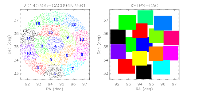
Figure 2: Spatial distribution of stars targeted by an example LSS-GAC plate 20140305-GAC094N35B1 (left) and the layout of the 16 rectangular boxes that are used to define the parent photometric samples from the XSTPS-GAC catalogue for the 16 spectrographs of LAMOST (right; see text for detail). In the left panel, stars targeted by different spectrographs are plotted with different colours. The spectrograph IDs are labelled. In the right panel, the rectangles are plotted with the same colour as the stars in the spectrographs they represent on the left.

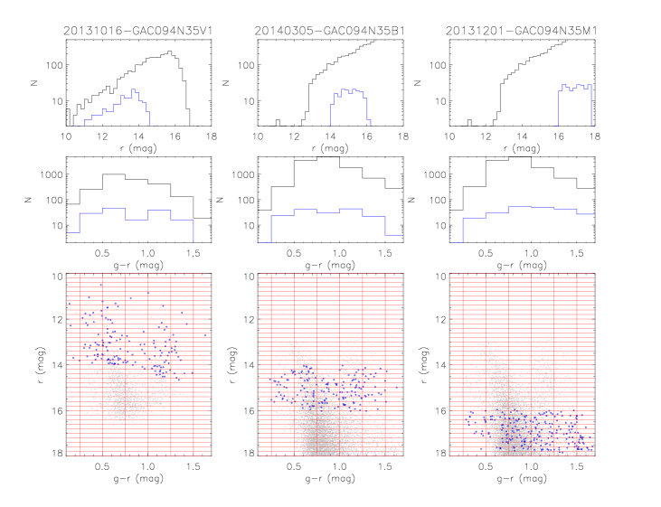
Figure 3: Distributions in CMDs of stars targeted by Spectrograph #1 of three example plates (blue dots and histograms) and of all stars in the representative rectangular box, for the case of using the APASS (left panel, a VB plate) or the XSTPS-GAC (middle panel, a B plate and right panel, an M plate) photometric catalogues. Red lines in the bottom panels show the grid of bins for $S_{1}$ evaluation. The observational dates and IDs of the three example plates are labeled at the top of the three columns.

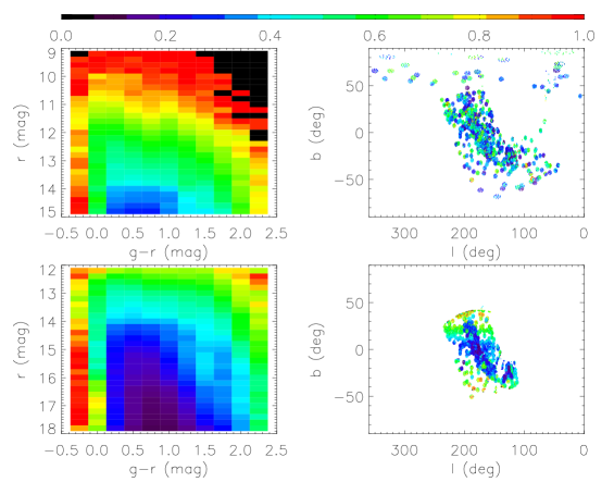
Figure 4: Distributions of mean values of $S_{1}$ in CMDs (left panels) and in Galactic longitude-latitude ($l~{},b$) plane (right panels) for stars targeted by all spectrographs of all plates included in the LSS-GAC DR2. The upper and bottom panels represent respectively results obtained using the APASS and XSTPS-GAC photometric catalogues.

We first collect all spectroscopic measurements in LSS-GAC. For those measurements, the selection effects come from the LSS-GAC target selection algorithm, i.e. $S_{1}$. We calculate $S_{1}$ for the individual spectrographs of each LSS-GAC plate. In Fig. 2, we show the spatial distribution in the sky for the measurements in different spectrographs of a given LSS-GAC plate. The boundaries of the individual spectrographs are irregular and the areas covered by them differ from each other. To make a robust comparison between the LSS-GAC targeted sample and the parent photometric sample, we consider each plate to be composed of rectangles, roughly centred on each spectrograph. The area of the rectangle is chosen to cover the same area in the sky as the corresponding spectrograph. Thus the stellar distribution in the rectangular area would be the same as that in the corresponding spectrograph, which can be used to calculate $S_{1}$. The centre of the rectangular area is set to the mean position of all stars targeted in the spectrograph. The size in Declination of the rectangular area is set to 1.1°, while the size in Right Ascension is set to $\Omega/(1.1\cos\delta)$, where $\Omega$ is the size of the spectrograph (unit in deg² ) and $\delta$ the central Declination of the spectrograph. We show in the right panel of Fig. 2 the rectangular areas for the individual spectrographs.

A LAMOST plate has a circular FoV of $\sim$20 deg, covering a diameter of 5 deg. Thus the individual spectrographs have an average area of $\sim$ 1.2 deg², comparable to the size of the box that we used for target selection (1° $\times$ 1°). According to the LSS-GAC target selection strategy, for the individual spectrographs of LAMOST, the probability of a star in a given colour-magnitude bin that is selected and gets observed by LAMOST, $S_{1}$, can be calculated as,

$$S_{1}=\dfrac{N_{\rm LAMOST}({\rm sp},C,M)}{N_{\rm phot.}({\rm sp},C,M)},$$ (1)

where ${N_{\rm LAMOST}({\rm sp},C,M)}$ and ${N_{\rm phot.}({\rm sp},C,M)}$ are respectively the number of all LAMOST measurements and the number of all photometric stars in a given colour $C$ and magnitude $M$ bin for Spectrograph sp of a LSS-GAC plate. For both the calculation with XSTPS-GAC and APASS photometric catalogues, $C$ and $M$ corresponds to $g-r$ and $r$, respectively. We adopt a colour and magnitude bin-size of $\delta(g-r)$ = 0.25 mag and $\delta r$ = 0.2 mag. Fig. 3 shows the colour and magnitude distributions of all targets observed with LAMOST and of the underlying photometric samples, along with the grid we use to calculate $S_{1}$, for Spectrograph #1 of three example plates.

The distributions of averaged values of $S_{1}$ in the CMD and in the Galactic longitude-latitude $(l,b)$ plane for targets observed with all spectrographs of all plates included in the LSS-GAC DR2 are shown in Fig. 4 for the cases of selection with APASS and selection with XSTPS-GAC. In general, brighter stars have higher values of $S_{1}$ than the fainter ones, and stars of extreme colours have higher values of $S_{1}$ than those of medium colours. The result is consistent with the strategy of LSS-GAC target selection, i.e., selecting stars uniformly and randomly from the CMDs. Stars of fainter magnitudes or of medium colours are much more numerous than those of brighter magnitudes or of extreme colours, so they have lower probabilities to get observed, i.e. smaller values of $S_{1}$. Spectrographs (of plates) of high Galactic latitudes have higher average values of $S_{1}$ than those of lower latitudes. Again, this is simply due to the steep decline of stellar number density (to a given limited magnitude) with latitude.

Note that there exists substantial overlaps between adjacent LSS-GAC plates. In addition, often there are more than two plates targeting the same field, covering exactly the same sky area. Nevertheless, it is extremely important to bear in mind that values of $S_{1}$ calculated here are for stars targeted by individual (plate) observations of LAMOST. For any follow-up scientific applications, e.g. to derive the underlying stellar number density of a given age from the LAMOST spectroscopic sample with robust stellar parameter determinations, results from the individual observations can only be combined after correcting for the selection effects.

3.2 Selection effect due to observation, data reduction and parameter determination

Table 1: Probabilities $S_{1}$, $S_{2}$ and $S$ for measurements catalogued in the LSS-GAC DR2.

Spec_id	Date	Plate	Spectrograph	RA	Dec	$S_{1}$	$S_{2}$	$S$	Notesa
20110921-PM1-01-003	20110921	PM1	01	12.90091	35.61838	0.100	0.600	0.060	1
20110921-PM1-01-005	20110921	PM1	01	13.23111	35.65357	0.154	0.833	0.128	1
20110921-PM1-01-006	20110921	PM1	01	12.98870	35.79328	0.182	1.000	0.182	1
20110921-PM1-01-007	20110921	PM1	01	13.24852	35.89709	0.750	1.000	0.667	1
…	…	…	…	…	…	…	…	…	…
20110921-PM1-01-011	20110921	PM1	01	13.18381	35.87553	0.062	1.000	0.062	2
20110921-PM1-01-013	20110921	PM1	01	12.93216	35.62636	0.571	0.750	0.429	2
…	…	…	…	…	…	…	…	…	…

^a 1: The probabilities calculated with the XSTPS-GAC photometric catalogue. 2: The probabilities calculated with the APASS photometric catalogue.

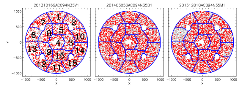
Figure 5: Spatial distributions of stars in the LAMOST focal plane (X, Y). The stars with reliable parameters determined with LSP3 are denoted with red dots. All stars selected and observed by LAMOST are denoted with grey dots. The three panels are corresponding to three example plates (a VB, a B and an M plate from left to right). The boundaries of the individual spectrographs are delineated by blue lines with IDs marked. The observational dates and IDs of the three plates are labelled on the top of the panels.

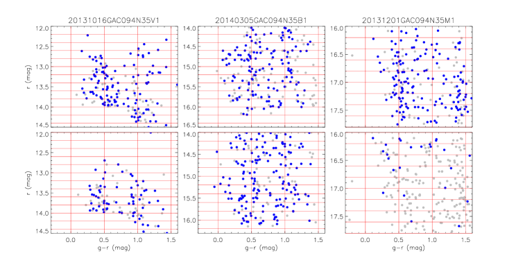
Figure 6: CMDs for stars observed with two selected spectrographs of three example plates. In each panel all stars selected and get observed with LAMOST (grey dots) and those with reliable parameters determined with LSP3 (blue dots) are shown. Values of colour $g-r$ and magnitude $r$ are from the XSTPS-GAC catalogue. Red lines delineate the grid of bins for $S_{2}$ evaluation. The observational dates and IDs of the plates are labelled on the top of the columns. The upper and bottom panels are for Spectrograph #15 and #6 of those plates, respectively.

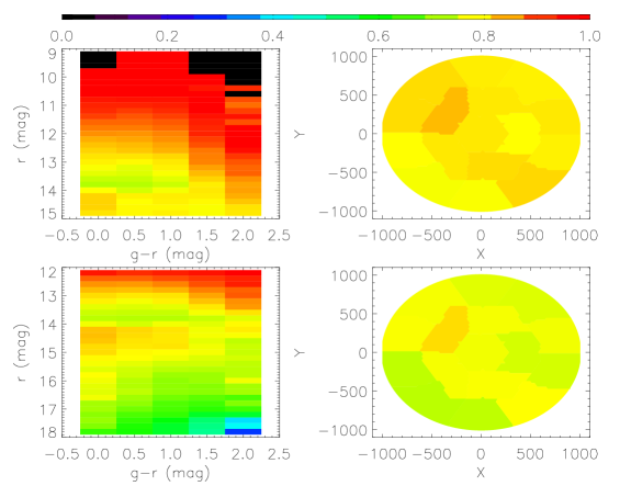
Figure 7: Distribution of averaged values of $S_{2}$ in the colour and magnitude $(C,~{}M)$ space (left panels) and in LAMOST focal plane ($X~{},Y$) (right panels) for all spectroscopic measurements with robust stellar parameters in LSS-GAC DR2. The top and bottom panels represent the results obtained using the APASS and XSTPS-GAC catalogues, respectively.

$S_{1}$ represents the bias induced by the LSS-GAC target selection algorithm. Accounting for $S_{1}$ will eliminate the discrepancy between the number of stars targeted by LAMOST and the number of stars in the parent photometric catalogue. However, there are additional effects that determine whether a spectroscopic measurement of star targeted by LAMOST ends up in the resultant spectroscopic catalogue with robust parameters. This is related to the quality of the observation, data reduction, and parameter determination. Robust estimates of stellar parameters, including radial velocities and basic atmospheric parameters, plus any additional information, such as values of interstellar extinction and distances can only be deduced from spectra of sufficient quality. Even for spectra of good quality, the currently developed stellar parameter pipelines (e.g. LSP3) may fail to deliver usable parameters because of lack of suitable analysis tools. This is the case for stars of extremely hot or cool colours. Thus one needs another quantity to account for this selection effect.

The precision of stellar parameters deduced from the spectra are mainly determined by the quality of spectra. The requirements are however different for different parameters. For example, robust radial velocities can be deduced for LAMOST spectra of $\rm SNR(4650\,\AA)$$>$5; while [$\alpha$/Fe] ratios can only be used for spectra of $\rm SNR(4650\,\AA)$$>$20 (Xiang et al., 2017a). Thus the selection criteria to build a spectroscopic sample with ‘robust’ parameters are different for different applications. In the current work, we consider a commonly used sample selected from the LSS-GAC DR2, following the recommendation of Xiang et al. (2017a). We select stars that have,

1. snr_b $>$ 10 for LAMOST spectra of good quality;

2. moondis $>$ 30 to avoid moonlight contamination;

3. vr_flag $\leq$ 6 and Teff $>$ 0 for robust radial velocity and atmospheric parameters;

4. satflag $=$ 0 to avoid CCD saturation;

5. brightflag $=$ 0 to eliminate contaminations by nearby bright stars;

6. deadfiber $=$ 0 to reject the spectra from LAMOST bad fibres;

The above criteria are the basic requirements for robust radial velocity and basic atmospheric parameters. We compare in Fig. 5 the distributions of stars observed with LAMOST and those with reliable parameters in the LAMOST focus physical plane ($X,~{}Y$) for three example plates. A similar comparison for two example spectrographs of the above three example plates is given in Fig. 6 in the colour-magnitude ($C,~{}M$) plane. It is clear that the probabilities of stars with reliable parameters depend on the spectrographs, plates with which they are observed, as well as on colours and magnitudes of the stars themselves.

As described above, whether a LAMOST spectrum is capable of delivering reliable stellar parameters could depend on many factors. The most important factor is of course the SNR of the spectrum that depends on the brightness of the target, the exposure time and the observation conditions. The individual spectrographs of LAMOST also have different throughputs (Yuan et al., 2015). Finally, the current implemented version of LSP3 pipeline uses the blue-arm spectra for parameter estimation. Thus stars of blue colours are more likely to yield spectra of sufficient SNRs and thus reliable stellar parameters than stars of red colours, either intrinsically red or heavily reddened by the interstellar dust grains. The quantity to account for all the above effects, $S_{2}$, defined above as the probability of a LAMOST spectrum of a star in a given colour-magnitude bin that is capable of delivering robust stellar parameters, can be calculated as,

$$S_{2}=\dfrac{N_{\rm PARAM}({\rm sp},C,M)}{N_{\rm LAMOST}({\rm sp},C,M)},$$ (2)

where ${N_{\rm PARAM}({\rm sp},C,M)}$ and ${N_{\rm LAMOST}({\rm sp},C,M)}$ are respectively the number of stars having reliable parameters in a colour-magnitude bin and the number of all stars in the same colour-magnitude bin that are selected and observed by LAMOST in Spectrograph sp of a given plate. Again, for both selection with the XSTPS-GAC and APASS catalogues, $C$ is $g-r$ and $M$ is $r$. The magnitude bin-size is the same ($\delta r$ = 0.2 mag) as in calculating $S_{1}$. We adopt however a larger colour bin-size [$\delta(g-r)$ = 0.5 mag] for calculating $S_{2}$ as this quantity is less sensitive to the colours of stars. In Fig. 6 we show the adopted colour-magnitude grid for some example spectrographs of three illustrative plates.

The distribution of averaged values of $S_{2}$ in the $C$-$M$ space and in the LAMOST focal plane for all spectroscopic measurements with robust stellar parameters in LSS-GAC DR2 are shown in Fig. 7. Bright and blue stars have higher averaged values of $S_{2}$ than faint and red stars. The differences in the average values of $S_{2}$ of the individual spectrographs are clearly visible, although the differences reduce significantly after averaging over all LSS-GAC plates. For example, Spectrographs #12 and #13 near the edge of the LAMOST focal plane have lower averaged values of $S_{2}$ (i.e. lower observing efficiencies) than Spectrographs #4 and #8 near the centre of the focal plane. The differences between the average values of $S_{2}$ of the individual spectrographs are more pronounced for results based on the XSTPS-GAC catalogue than those based on the APASS catalogue, with the fraction of faint (B/M) plates are larger in the former case.

3.3 The final selection function

In the case that both $S_{1}$ and $S_{2}$ are evaluated using the same $C$ and $M$ bin sizes, then the final selection function, $S$, is simply given by the product of $S_{1}$ and $S_{2}$. However, as noted above, we use slightly different $C$ and $M$ bin sizes when evaluating $S_{2}$ compared to the bin sizes used for $S_{1}$. As such, we now define $C1$ and $M1$ for the colour-magnitude bin used to calculate $S1$. Similarly, $C2$ and $M2$ is defined as the colour-magnitude bin used to calculate $S2$. The final selection function, $S$, is given by

$$S=\dfrac{N_{\rm PARAM}({\rm sp},C2,M2)}{N_{\rm total}({\rm sp},C2,M2)},$$ (3)

where for each spectrograph ${\rm sp}$ and each $C2$ and $M2$ bin, $N_{\rm PARAM}({\rm sp},C2,M2)$ is the number of stars having robust parameters and $N_{\rm total}({\rm sp},C2,M2)$ is the total number of stars observed by LAMOST with target selection function $S_{1}$ corrected. We thus have

$$N_{\rm total}({\rm sp},C2,M2)={\sum\limits_{C1\in C2}\sum\limits_{M1\in M2}\frac{N_{\rm LAMOST}({\rm sp},C1,M1)}{S_{1}({\rm sp},C1,M1)}}.$$ (4)

Example values of selection functions $S_{1}$, $S_{2}$ and $S$ thus calculated for spectroscopic measurements in LSS-GAC DR2 are given in Table 1 for the purpose of illustration. The full results are available by contacting the authors (BQC, XWL) and will be included in the next release of LSS-GAC value-added catalogue, i.e. LSS-GAC DR3 (Huang et al., in preparation).

4 Mock data test

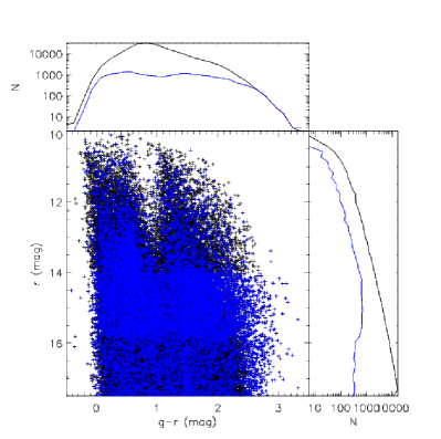
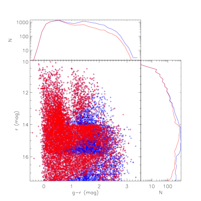
Figure 8: Top panel shows distributions in colour-magnitude plane of targets selected from the Besançon simulated catalogue (black dots and histograms), using the same target selection algorithm as for LSS-GAC (blue dots and histograms). Selected targets with simulated ‘SNR’ $>$ 10 (see text for details) are represented by red dots and histograms in the bottom panel.

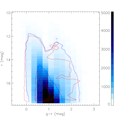
Figure 9: Hess diagram of the mock ‘photometric’ sample (blue scales and contours), compared to that given by the sample with ‘reliable’ parameters after corrected for the selection biases (red contours).

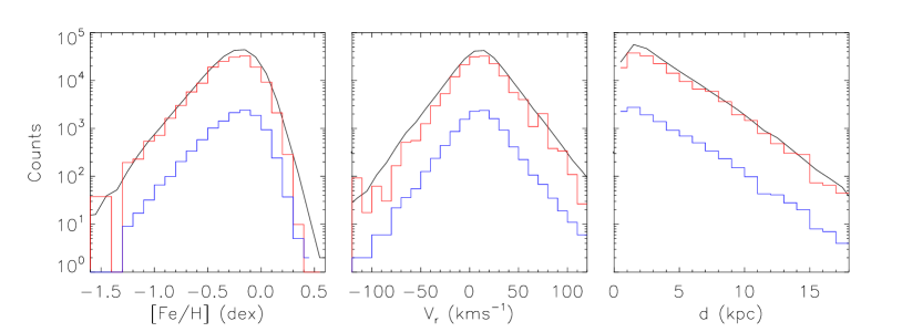
Figure 10: Distributions of metallicity [Fe/H], radial velocity $V_{\rm r}$ and distance $d$ for the mock ‘photometric’ sample (black histograms), the sample with ‘reliable’ parameters (blue histograms), and for the sample with ‘reliable’ parameters after corrected for the selection effects (red histograms).

In this Section we validate our method using a mock star catalogue. For this purpose, we utilise the Besançon stellar population synthesis model (Robin et al., 2003) to generate a catalogue centred on the GAC, ($l,~{}b$) = (180°, 0°). The three-dimensional extinction maps from Chen et al. (2014) are used to add extinction to stars in the catalogue. Taking the simulated catalogue as an observed one, we select targets using the same algorithm as adopted for the LSS-GAC target selection. We artificially define a field centred on ($l,~{}b$) = (180°, 0°). Within this field, four plates, one VB, two B and one M plates, are generated, containing 4 000, 3 888, 3 914 and 3 950 stars, respectively. In Fig. 8 we plot the colours and magnitudes of the selected targets, along with those of all stars in the full ‘photometric’ catalogue.

To define a sample of stars with ‘reliable stellar parameters’, we artificially add SNRs to all of the selected targets. To simulate the quality of stellar spectra in real LAMOST observations, we randomly select three plates from LSS-GAC: a VB plate HD213239N421743V01, a B plate GAC101N22B1 and an M plate GAC091N33M1. For each spectrograph of each plate, the distribution of $\rm SNR(4650\,\AA)$ of stars in the selected plates is fitted as a function of colour $g-r$ and magnitude $r$, as,

$${\rm SNR}=a_{1}+a_{2}(g-r)+a_{3}(g-r)^{2}r+a_{4}(g-r)r+a_{5}r+a_{6}r^{2},$$ (5)

where $a_{1}$, $a_{2}$, …, and $a_{6}$ are the coefficients. The fitting is then applied to all spectrographs of simulated plates to assign ‘real’ SNRs for those selected and get ‘observed’ stars. We ignore here the effects of the dead, saturated or contaminated fibres and the uncertainties induced by the LSP3 pipeline. Assuming that the LSP3 pipeline is able to deliver robust stellar parameters for all stars with a ‘SNR’ $>$ 10, the sample of stars with robust parameters is simply defined by stars with a ‘SNR’ $>$ 10. In Fig. 8, stars in this sample with ‘robust’ parameters are also overplotted.

We now have a ‘photometric’ sample generated with the Besançon model, a sample of stars selected with the same target selection algorithm as for the LSS-GAC and get ‘observed’, and a sample with ‘reliable’ parameters by adding artificially ‘SNRs’ to their ‘observed’ spectra. The values of selection function for each star with ‘reliable’ parameters are then calculated following the procedure introduced in the former Section.

The sample with ‘reliable’ parameters is then corrected for selection biases using the calculated selection function. In Fig. 9, we compare the resultant colour and magnitude distribution of the sample with ‘reliable’ parameters after correcting for the selection effects with the distribution of the underlying population (i.e. the ‘photometric’ sample). Overall the agreement is quite good. For regions of extreme red colours and faint magnitudes, given the small number of stars with ‘reliable’ parameters, we are not able to perfectly recover the CMD of the underlying stellar population.

We have also tested our selection function results for the metallicity, radial velocity and star count distributions. Comparisons of those distributions as given the sample with ‘reliable’ parameters after corrected for the selection effects and those of the underlying population are shown in Fig. 10. Overall, the agreement is good. We note that for stars of extreme parameters, such as those of very high metallicities, very high radial velocities, or very far distances, due to the large statistical uncertainties, the two sets of distributions do not match well, but are still consistent with each other. Thus the selection function presented in the current work is a powerful tool for the studies of Galactic chemistry and dynamics.

5 Applications of the selection function

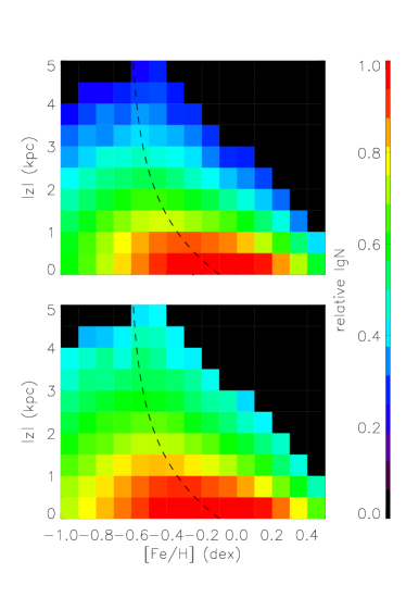
Figure 11: Distribution of stellar number density in the metallicity [Fe/H] and height from the Galactic mid-plane $|z|$ from a sample of LAMOST F-type stars. The density is shown on a logarithmic scale, with peak value normalized to unity. The dashed lines show Eq. (11) of Chen et al. (2017). The top and bottom panels show results before and after applying the selection function corrections, respectively.

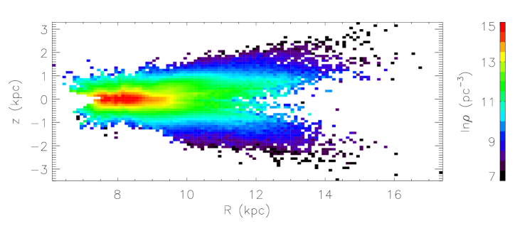
Figure 12: Stellar density distribution in the $R$ - $z$ plane deduced from a sample of LAMOST F-type stars after corrected for selection biases. The colour encodes the mean ln $\rho$ value in each $R$-$z$ bin.

In this Section we give two simple applications of our selection function. We select a sample of F-type stars from the internal release of LSS-GAC DR2 with effective temperature and surface gravity cuts, 6000 $<$ $T_{\rm eff}$ $<$ 6800 K and 3.8 $<$ log $g$ $<$ 5.0 dex. The internal release of LSS-GAC DR2 includes all observations from the initiation of the survey up to 2016 June. The selected F-type star sample contains 713 016 spectroscopic measurements.

5.1 The metallicity distribution

In Fig. 11, we plot the distribution of stellar number density in the plane of metallicity [Fe/H] and height from the Galactic mid-plane $|z|$ of this sample for the metallicity and height ranges, $-$1 $<{\rm[Fe/H]}<$ 0.5 dex and 0 $<|z|<$ 5 kpc. The peak value of the distribution is normalized to unity. The upper and bottom panels show respectively the results derived before and after applying the selection function corrections deduced in the current work. When plotting the distributions, we have discarded bins containing fewer than 10 stars. For different $|z|$ slices, the variations of peak metallicities as a function of $|z|$ is consistent with the fit given by Eq. (11) of Chen et al. (2017), a fit obtained using main sequence turn off stars selected from LSS-GAC DR2 (Xiang et al., 2015b). The variations of peak metallicities as $|z|$ are quite similar before and after applying the selection function corrections, suggesting that the LSS-GAC selection function has only a marginal effect on the metallicity peak distributions. This is in consistent with the recent work by Nandakumar et al. (2017).

Amongst the individual $|z|$ slices, both the metallicity dispersion and skewness vary. As $|z|$ increases, the metallicity dispersions decrease while the skewness increase, which imply the star formation and radial migrations history of the Galactic thin and thick disks (Sellwood & Binney, 2002; Schönrich & Binney, 2009; Hayden et al., 2015; Loebman et al., 2016). A detailed analysis of the Galactic disk metallicity distribution based on the LAMOST main sequence turn off stars will be presented in a separate work (Wang et al., in preparation). Compared to the distributions after the selection effect corrections, those before the selection function corrections have smaller dispersions and larger skewness. This is likely to be caused by the fact that stars further away (of larger $|z|$) are fainter and thus suffer from larger selection effects than those nearby ones.

5.2 The stellar number density distribution

Fig. 11 also shows for different metallicity bins how the stellar number density varies with $|z|$. It is clear that the number densities of metal-poor populations decrease more slowly than those of the metal-rich ones, in other words, the metal-poor populations have larger scale heights. There is no doubt that applying the selection function corrections is very important for this type of study. Without the corrections, the scale heights derived will be systematically underestimated. This is again largely due to the fact that stars further away suffer from larger selection effects than those nearby.

With the selection function corrections presented here, one can thus examine the underlying stellar number density distributions using the LAMOST spectroscopic samples. We give an example here using the F-type star sample. From stars observed in each spectrograph of each plate, one can simply derive the stellar number density using,

$$\rho_{j}=\dfrac{\Sigma_{i,j}(\frac{1}{S_{i,j}})}{V_{j}},$$ (6)

where $i$ is the index of stars in a distance bin of index $j$, and $V_{j}$ is the volume of the $j$th distance bin. We adopt the centre $l$ and $b$ for each spectrograph and convert ($l,~{}b,~{}d$) into the Galactocentric cylindrical coordinates ($R,~{}z,~{}\phi$) similar as in Bovy et al. (2012) and Liu et al. (2017). The resultant number density is then averaged in the $R$ and $z$ plane. The results are presented in Fig. 12. The Figure displays a remarkable shape of the Galactic disk, very similar to that seen in an edge-on external disk galaxy, for Galactic radius $R$ between 5 and 16 kpc. Note that here we have assumed that the photometric sample from which LAMOST targets are drawn is complete. In addition, we have also ignored the possible variations of the absolute magnitudes of F-type stars. Any such variations, coupled with the varying interstellar extinction, affect the lower and upper completeness distance limits for the individual lines of sight lines, effects that one must take into account when studying the Galactic structure (Chen et al., 2017). More quantitative analysis will be presented in a separate work ( Chen et al., in preparation).

6 Summary

In this paper, we have discussed in detail the selection function of LSS-GAC spectroscopic survey and presented corrections for all spectroscopic measurements with reliable parameters in the LSS-GAC DR2. The selection function determines how representative the final spectroscopic catalogue is compared to the underlying stellar population of the Milky Way. It is a powerful tool for the studies of the Galactic chemistry and structure problems.

We divide the selection function into two parts. The first part, quantified by $S_{1}$, characterise the LSS-GAC target selection strategy. The LSS-GAC target selection is based on stellar magnitudes and colours, using photometric data from the XSTPS-GAC, supplemented by PPMXL and 2MASS photometry for the VB survey. Based on the photometric data of XSTPS-GAC and APASS DR9, we calculate $S_{1}$ in the $C$ and $M$ space for each spectrograph of each LSS-GAC plate. The second part, quantified by $S_{2}$, characterise the selection effects due to the observational quality, data reduction and parameter determination. We select from LSS-GAC DR2 a commonly used sample that contains stars with reliable stellar parameters. Values of $S_{2}$ of the sample are calculated for each $C$-$M$ bin and for each spectrograph of each plate. The full selection function $S$ can then be calculated from $S_{1}$ and $S_{2}$. Example values of selection function corrections are listed in Table 1. The full results are available upon request by email, and will be included in the next release of LSS-GAC value-added catalogue.

We test our method using mock data. The test shows that the selection function corrections presented here can successfully recover the distributions of colours, magnitudes, metallicities, radical velocities, as well as number counts of the underlying stellar populations. Finally we present two simple applications of our deduced selection function corrections. The selection function presented in the current work provide a better insight of the properties of LSS-GAC and the resulted value-added catalogue, and can be used to study a variety of problems of the Milky Way galaxy that rely on proper corrections for the selection biases in the LSS-GAC spectroscopic dataset.

References

- Bovy et al. (2012) Bovy, J., Rix, H.-W., Liu, C., Hogg, D. W., Beers, T. C., & Lee, Y. S. 2012, ApJ, 753, 148
- Chen et al. (2017) Chen, B.-Q., et al. 2017, MNRAS, 464, 2545
- Chen et al. (2014) Chen, B.-Q., et al. 2014, MNRAS, 443, 1192
- Cheng et al. (2012) Cheng, J. Y., et al. 2012, ApJ, 746, 149
- Deng et al. (2012) Deng, L.-C., et al. 2012, Research in Astronomy and Astrophysics, 12, 735
- Gilmore et al. (2012) Gilmore, G., et al. 2012, The Messenger, 147, 25
- Hayden et al. (2015) Hayden, M. R., et al. 2015, ApJ, 808, 132
- Henden et al. (2016) Henden, A. A., Templeton, M., Terrell, D., Smith, T. C., Levine, S., & Welch, D. 2016, VizieR Online Data Catalog, 2336
- Liu & van de Ven (2012) Liu, C. & van de Ven, G. 2012, MNRAS, 425, 2144
- Liu et al. (2017) Liu, C., et al. 2017, Research in Astronomy and Astrophysics, 17, 096
- Liu et al. (2014) Liu, X.-W., et al. 2014, in IAU Symposium, Vol. 298, Setting the scene for Gaia and LAMOST, ed. S. Feltzing, G. Zhao, N. A. Walton, & P. Whitelock, 310–321
- Liu et al. (2015) Liu, X.-W., Zhao, G., & Hou, J.-L. 2015, Research in Astronomy and Astrophysics, 15, 1089
- Loebman et al. (2016) Loebman, S. R., Debattista, V. P., Nidever, D. L., Hayden, M. R., Holtzman, J. A., Clarke, A. J., Roškar, R., & Valluri, M. 2016, The Astrophysical Journal Letters, 818, L6
- Luo et al. (2012) Luo, A.-L., et al. 2012, Research in Astronomy and Astrophysics, 12, 1243
- Luo et al. (2015) Luo, A.-L., et al. 2015, Research in Astronomy and Astrophysics, 15, 1095
- Majewski et al. (2015) Majewski, S. R., et al. 2015, ArXiv 1509.05420
- Nandakumar et al. (2017) Nandakumar, G., Schultheis, M., Hayden, M., Rojas-Arriagada, A., Kordopatis, G., & Haywood, M. 2017, A&A, 606, A97
- Nidever et al. (2014) Nidever, D. L., et al. 2014, ApJ, 796, 38
- Rebassa-Mansergas et al. (2015) Rebassa-Mansergas, A., et al. 2015, MNRAS, 450, 743
- Robin et al. (2003) Robin, A. C., Reylé, C., Derrière, S., & Picaud, S. 2003, A&A, 409, 523
- Roeser et al. (2010) Roeser, S., Demleitner, M., & Schilbach, E. 2010, AJ, 139, 2440
- Schlesinger et al. (2012) Schlesinger, K. J., et al. 2012, ApJ, 761, 160
- Schönrich & Binney (2009) Schönrich, R. & Binney, J. 2009, MNRAS, 396, 203
- Sellwood & Binney (2002) Sellwood, J. A. & Binney, J. J. 2002, MNRAS, 336, 785
- Skrutskie et al. (2006) Skrutskie, M. F., et al. 2006, AJ, 131, 1163
- Steinmetz et al. (2006) Steinmetz, M., et al. 2006, AJ, 132, 1645
- Stonkutė et al. (2016) Stonkutė, E., et al. 2016, MNRAS, 460, 1131
- Wojno et al. (2017) Wojno, J., et al. 2017, MNRAS, 468, 3368
- Wu et al. (2014) Wu, Y., Du, B., Luo, A., Zhao, Y., & Yuan, H. 2014, in IAU Symposium, Vol. 306, Statistical Challenges in 21st Century Cosmology, ed. A. Heavens, J.-L. Starck, & A. Krone-Martins, 340–342
- Wu et al. (2011) Wu, Y., et al. 2011, Research in Astronomy and Astrophysics, 11, 924
- Xiang et al. (2017a) Xiang, M.-S., et al. 2017a, MNRAS, 464, 3657
- Xiang et al. (2015a) Xiang, M. S., et al. 2015a, MNRAS, 448, 822
- Xiang et al. (2015b) Xiang, M.-S., et al. 2015b, Research in Astronomy and Astrophysics, 15, 1209
- Xiang et al. (2017b) Xiang, M.-S., et al. 2017b, MNRAS
- Xiang et al. (2015c) Xiang, M. S., et al. 2015c, MNRAS, 448, 90
- Yanny et al. (2009) Yanny, B., et al. 2009, AJ, 137, 4377
- Yuan et al. (2015) Yuan, H.-B., et al. 2015, MNRAS, 448, 855
- Zhang et al. (2014) Zhang, H.-H., Liu, X.-W., Yuan, H.-B., Zhao, H.-B., Yao, J.-S., Zhang, H.-W. Xiang, M.-S., & Huang, Y. 2014, Research in Astronomy and Astrophysics, 14, 456
- Zhao et al. (2012) Zhao, G., Zhao, Y.-H., Chu, Y.-Q., Jing, Y.-P., & Deng, L.-C. 2012, Research in Astronomy and Astrophysics, 12, 723