Entanglement entropy between virtual and real excitations in quantum electrodynamics

Abstract

The aim of this work is to introduce the entanglement entropy of real and virtual excitations of fermion and photon fields. By rewriting the generating functional of quantum electrodynamics theory as an inner product between quantum operators, it is possible to obtain quantum density operators representing the propagation of real and virtual particles. These operators are partial traces, where the degrees of freedom traced out are unobserved excitations. Then the Von Neumann definition of entropy can be applied to these quantum operators and in particular, for the partial traces taken over the internal or external degrees of freedom. A universal behavior is obtained for the entanglement entropy for different quantum fields at zero order in the coupling constant. In order to obtain numerical results at different orders in the perturbation expansion, the Bloch-Nordsieck model is considered, where it it shown that for some particular values of the electric charge, the von Neumann entropy increases or decreases with respect to the non-interacting case.

1 Introduction

Entanglement entropy has become an important topic in theoretical physics and has become a widely studied topic in the last few years. In general, the entanglement is studied between one part of a system and in different branches of theoretical physics usually the partitioning is spatial. An entanglement entropy can be defined through the quantum density operator and permits applying the concept in different frameworks, for example to distinguish new topological phases and characterize critical points ([1], [2] and [3]) or in discussions of holographic descriptions of quantum gravity, in particular, for the AdS/CFT correspondence ([4]). More recently the entanglement entropy has been applied in condensed matter physics, density matrix renormalization group method ([5], [6]) and black hole thermodynamics (see [7], [8], [9], [4], [10] and [11]), thermal quantum field theory (see [12], [13] and [14]) curved space-time (see [15], [16] and [17]), decoherence [18], squeezed vacuum [19] and in low dimension systems [20].

The concept of entanglement entropy in quantum field theory is linked to a region of space-time that contains the relevant degrees of freedom ([21], [22], [23] and [24]). The trace over the degrees of freedom localized on a region which is not accessible to the observer, results in a reduced density matrix. Then, the von Neumann definition of entanglement entropy can be applied to obtain a measure of the inaccesibility of the vacuum state that is mixed after the partial trace. In QFT geometric entropy can be computed by using the Euclidean path integral method in models without interactions and the results show that in $d$ dimensions, the entropy behaves as a Laurent series starting in $\epsilon^{-(d-1)}$, where $\epsilon$ is a short-distance cutoff and the leading coefficient that multiplies to $\epsilon^{-(d-1)}$ is proportional to the $d-1$ power of the size of $V$, which is the area law for the entanglement entropy [9].

Although entanglement entropy in quantum field theory has been focused on entanglement between degrees of freedom associated with spatial regions, it is also permissible to consider the entanglement between real and virtual excitations. The virtual excitations are a mere mathematical artifact of the pertubation expansion, so in principle any physical quantity that depends on this entanglement depends naturally on interactions introduced in the Lagrangian. On the other hand, given that interactions introduce virtual excitations and these are entangled with the real excitations, then an interaction entanglement entropy can be defined and it would be a measure of the information restored in the propagation of the quantum field, this information would depend on the interactions with other quantum fields or itself. In [25], the generating functional of the $\phi^{4}$ theory has been written in terms of quantum operators. These operators are partial traces over larger quantum operators that depends on the internal vertices and a new set of vertices. These new vertices imply that there are real particles propagating elsewhere but cannot be measured; then we must average over the possible space-time points where these particles propagate. This inaccesibility to these new particles implies that there are unobserved particles or virtual particles. That is, interactions introduce new particles, but these particles cannot be observed, then the quantum state must be traced out. Because the real particles and the new particles are entangled, then the entanglement entropy can be computed. A very simple example (see [25]) is the first order correction to the $\phi^{4}$ theory, where the quantum density operator can be written as (not normalized)

$$\rho=\int\Delta(x_{1}-y_{1})\Delta(y_{1}-w_{1})\Delta(y_{1}-x_{2})\left|x_{1},y_{1}\right\rangle\left\langle x_{2},w_{1}\right|d^{4}w_{1}d^{4}y_{1}d^{4}x_{1}d^{4}x_{2}$$ (1)

By considering the following quantum operator

$$O=\int\delta(y_{1}-w_{1})J(x_{1})J(x_{2})\left|x_{1},y_{1}\right\rangle\left\langle x_{2},w_{1}\right|d^{4}w_{1}d^{4}y_{1}d^{4}x_{1}d^{4}x_{2}$$ (2)

where $J(x)$ are the external sources and the Dirac delta $\delta(y_{1}-w_{1})$ is explicitly shown inside the integral in order to remark that the coefficients related to the internal degrees of freedom are the identity matrix. Then it follows that the mean value $Tr(\rho O)$ is identical to the first order in $\lambda_{0}$ of the generating functional. In turn, $Tr(\rho O)=Tr(\rho_{ext}O_{ext})$, where

$$\rho_{ext}=Tr_{int}(\rho)=\Delta(0)\int\Delta(x_{1}-y_{1})\Delta(y_{1}-x_{2})d^{4}y_{1}\left|x_{1}\right\rangle\left\langle x_{2}\right|d^{4}x_{1}d^{4}x_{2}$$ (3)

which is identical to the first correction to the two-point correlation function. The trace over the internal degrees of freedom $y_{1}$ and $w_{1}$ implies that there is a virtual propagation between $y_{1}$ and $w_{1}$ that is unobserved and then their degrees of freedom must be traced out. This is the crucial point of the idea of this manuscript and [25]: the quantum operator of the quantum field theory is a partial trace which implies, in some sense, that some physical process has been neglected and moreover, the consequences of this lack of observability occurs in the scattering processes of $\phi^{4}$ theory. The coefficient of the quantum density operator $\rho$ is entangled in the coordinates because these are linked through the propagators. Making a Fourier transform, the quantum operator can be written in the momentum basis as

$$\rho=\int\int\frac{d^{D}p}{(2\pi)^{D}}\frac{d^{D}q}{(2\pi)^{D}}\frac{d^{D}r}{(2\pi)^{D}}\frac{1}{p_{1}^{2}-m_{0}^{2}}\frac{1}{p_{2}^{2}-m_{0}^{2}}\frac{1}{p_{3}^{2}-m_{0}^{2}}\left|p_{1},p_{2}+p_{3}-p_{1}\right\rangle\left\langle p_{3},p_{2}\right|$$ (4)

In this way, the coefficient is not entangled, each propagator depends on its momentum vector but the entanglement has been translated to the bra and ket vectors. That is, the degrees of freedom of an interacting quantum field theory are entangled in momentum space [26].

In [27], [28] and [29], the full description of the model described above is done, where the intermediate operators introduced artificially by the perturbation expansion can be obtained as partial traces over the internal degrees of freedom, represented by a duplication of the internal vertices of the internal propagators. The particles that are created in these vertices are virtual particles because they do not obey the constraint of the energy-momentum relation. This implies that these particles are not measured, then it must be traced out. This unobservation causes these particles to become virtual. One of the most known consequence of the imposibility of unobserved particles is in the scattering process of quantum electrodynamics (QED), where the infrared divergences are canceled by the contribution of the soft photons which are unobserved photons ([30] and [31]). Although this phenomena will be discussed in the next section in relation with the photon entropy, it must be stressed that the additional soft photon emmisions can be interpreted as ”opened” loops in the scheme presented in [25] (figure 1). It should be stressed that in the previous work [25], the quantum operators $\rho$ and $O$ has been called ”states” and ”observables”. Although the main result of this work, where the correlation function can be written as $Tr(\rho O)$ suggests to consider $\rho$ as a quantum state written formally as a quantum density operator and $O$ as an observable, the mathematical objects cannot be associated to physical concepts, mainly because the latter can be constrained by physical relations, where the former are defined mathematically. In particular, the quantum states satisfy dynamical equations and the quantum density operators $\rho$ defined in [25] using the generating functional obeys a functional differential equation (see eq.(1) of page 288 of [32]). In this sense, the quantum entropy computed can be related to processes, but not to quantum states.

The model introduced in this work can be considered a particular case of the General Boundary Formalism (GBF) ([33], [34], [35], [36] and [37]), where to each boundary $S$ defined by an space-like hyperplane in Minskowski space-time there is a vector space $\mathcal{H}_{s}$. In turn, for a given boundary $S$ changing the orientation corresponds to replace $\mathcal{H}_{s}$ with $\mathcal{H}_{s}^{\ast}$. Moreover, associated with $M$, which is the region bounded by $S$, there is a complex function $\rho_{M}:\mathcal{H}_{s}\rightarrow\mathbb{C}$ which associates an amplitude to a state. In turn, if $S$ can be decomposed into disconnected componentes $S=S_{1}\cup S_{2}...\cup S_{n}$, then one may convert $\rho_{M}:\mathcal{H}_{S_{1}}\otimes...\otimes\mathcal{H}_{S_{n}}\rightarrow\mathbb{C}$ to a function $\rho_{M}:\mathcal{H}_{S_{1}}\otimes...\otimes\mathcal{H}_{S_{k}}\rightarrow\mathcal{H}_{S_{k+1}}^{\ast}\otimes...\otimes\mathcal{H}_{S_{n}}^{\ast}$ replacing spaces with dual spaces. In the general boundary formalism, then the focus is moved from quantum states, which describe a system at some given time, to quantum states of processes, which describe what happens to a local system during a finite time-span. For conventional nonrelativistic system, the quantum space of the processes are defined as the tensor product of the initial and final Hilbert state spaces $\mathcal{H}_{1}\otimes\mathcal{H}_{2}$ where the subscripts $1$ and $2$ indicate the initial and final stages of the process. The amplitude of the process is represented by the Feynman propagator and is determined as a linear functional over the quantum state defined as the tensor product of the initial and final quantum states. In [25], the processes are ordered in terms of the perturbation parameter $\lambda_{0}$. The external points of the correlation functions define the boundary and this boundary should be chosen as space-like hyperplanes as it is done in [36], which implies to fix the time components of $x_{1}$ and $x_{2}$ and consider $\mathcal{H}_{1}\otimes\mathcal{H}_{2}$ as the space which represents the whole family of transition amplitudes between two space-like hyperplanes. But when interactions are turned on, internal propagators appear and moreover, we must integrate over the possible space-time coordinate of these propagators. Must be stressed that to integrate in the external points, implies to connect $x_{1}$ with $x_{2}$ in the Feynman diagrams, which is a simple example of the generation of correlation functions from vacuum diagrams (see Section 5.5 of [38], page 68), where for example, by cutting one line to the first order vacuum diagram we obtain the first order contribution to the two-point function. Then, the space-time coordinates should not be fixed when interactions are considered because all the correlation functions are related. A vertex inside a Feynman diagram can be converted into an external point by cutting an internal propagator (see [25]). As an example of the concept of family of processes, we can consider the Feynman propagator in 3+1 dimensions (see [39])

$$\Delta(s)=\theta(s^{2})\frac{im}{8\pi\sqrt{s^{2}-i\epsilon}}H_{1}^{(2)}(m\sqrt{s^{2}-i\epsilon})+$$ (5)

$$\theta(-s^{2})\frac{im}{8\pi\sqrt{-s^{2}+i\epsilon}}K_{1}(m\sqrt{-s^{2}+i\epsilon})$$

where $s^{2}=\Delta t^{2}-\Delta r^{2}$ is the proper distance and $H_{1}^{(2)}$ is the Hankel function of the second kind and $K_{1}$ is the modified Bessel function of the first kind. What is interesting of this propagator is that depends on the proper distance between the two space-time coordinates. We can consider the whole family of processes that is parametrized by $s$. For $s\in(-\infty,0)$  we have spacelike interval, $s=0$ lightlike interval and $s\in(0,\infty)$ timelike interval. We can consider that we are only interested in those processes with timelike interval, then if we consider $\Delta(s)$ the amplitude of the process, then $\left|\Delta(s)\right|^{2}$ is the probability of the process. If we demand that it is a probability then it must be normalized, which can be obtained easily for timelike intervals $\int_{0}^{\infty}\left|\Delta^{2}(s)\right|ds=\frac{m^{3}}{2\pi^{3}}$ .

In [41], the distinction between pure and mixed states is weaken in the general covariant context when finite spatial regions are considered. In the model introduced in this paper, the quantum state is mixed when interactions are turned on. The mixture is due to the entanglement of the virtual state in the bulk with the real states in the boundary. In turn, for free fields there is a priori distinction between pure and mixture states because we can distinguish between past and future parts of the boundary. Moreover, the observables acts in the infinite past and infinite future. In this sense, it seems that the model introduced in the manuscript submitted is a particular case of the general boundary formalism with the incorporation of the interactions treated in a perturbative manner and allowing these virtual states to be defined in the whole space-time.

In order to introduce the formalism for quantum operators and where the trace can be applied, the generating functional of the quantum field theory must be considered. As it was done for the self-interacting theory $\phi^{4}$, it is necessary to establish the formalism to the quantum field theory of electrons, positrons and photons in order to apply the concept of entanglement entropy between these particles. Due to the complicated integrals that must be solved, in order to obtain results for the second order corrections to the photonic and fermionic entropies, the Bloch-Nordsieck model [42] will be considered, to show the way in which the interaction entanglement introduces changes in the quantum entropy. Then, the manuscript will be organized as follows: In Section II, the formalism for the quantum opearators by rewriting the generating functional is introduced for electrons and photons. In section III, the von Neumann entropy is computed for the electron and photon propagator at zero order in $e$ and the first corrections are sketched by using the results found in Appendix B. The Bloch-Nordsieck model is discussed and exact results for the von Neumann entropy are obtained. In last section, the conclusions are presented and in Appendix A a conceptual discussion of the model is done.

2 Quantum operators in QED

The generating functional can be constructed in a general way by considering some (symmetric) $n$-point functions $\tau^{(n)}(x_{1},...,x_{n})$, then the corresponding generating functional ([43], eq. (II.2.21), [44], eq. (3.2.11)) can be defined as

$$Z\left[\eta,\overline{\eta}\right]=\underset{n=0}{\overset{\infty}{\sum}}\frac{i^{n}}{n!}\int\tau^{(n)}(x_{1},...,x_{n})\eta(x_{1})\overline{\eta}(x_{2})...\eta(x_{n-1})\overline{\eta}(x_{n})\underset{i=1}{\overset{n}{\prod}}d^{4}x_{i}$$ (6)

where $\eta(x_{i})$ and $\overline{\eta}(x_{i})$ are external sources for $\psi(x_{i})$ and $\overline{\psi}(x_{i})$ fields respectively and $\tau^{(n)}$ can be

$$\tau_{F}^{(n)}(x_{1},...,x_{n}) = S^{(n)}(x_{1},...,x_{n})=\left\langle\Omega\left|\psi(x_{1})\overline{\psi}(x_{2})...\psi(x_{n-1})\overline{\psi}(x_{n})\right|\Omega\right\rangle$$ (7)

$$\tau_{P}^{(n)}(x_{1},...,x_{n}) = D_{\mu_{1},...,\mu_{n}}^{(n)}(x_{1},...,x_{n})=\left\langle\Omega\left|A_{\mu_{1}}(x_{1})...A_{\mu_{n}}(x_{n})\right|\Omega\right\rangle$$

where the first correlation function is for fermions and the second is for photons, $\psi(x)$ ($\overline{\psi}(x)$) and $A_{\mu}(x)$ are the fermion (positron) and photon fields and $\left|\Omega\right\rangle$ is the vacuum state. A convenient way to eliminate trivial contributions in the correlation function is by introducing a modified generating functional $Z\left[\eta,\overline{\eta}\right]$ for irreducible Green’s functions that is defined as $W\left[\eta,\overline{\eta}\right]=e^{iZ\left[\eta,\overline{\eta}\right]}$. The new generating functional $Z\left[\eta,\overline{\eta}\right]$ satisfies the normalization condition $Z[0,0]=0$ and it reads

$$Z\left[\eta,\overline{\eta}\right]=\underset{n=0}{\overset{\infty}{\sum}}\frac{1}{n!}\int\tau_{c}^{(n)}(x_{1},...,x_{n})\eta(x_{1})\overline{\eta}(x_{2})...\eta(x_{n-1})\overline{\eta}(x_{n})\underset{i=1}{\overset{n}{\prod}}d^{4}x_{i}$$ (8)

where in this case $\tau_{c}^{(n)}(x_{1},...,x_{n})$ are connected $n$-point functions that can be obtained by differentiation

$$\tau_{c}^{(n)}(x_{1},...,x_{n})=\frac{\delta^{n}Z\left[\eta,\overline{\eta}\right]}{\delta\eta(x_{1})\delta\overline{\eta}(x_{2})...\delta\eta(x_{n-1})\delta\overline{\eta}(x_{n})}\mid_{\begin{subarray}{c}\eta=0\\ \overline{\eta}=0\end{subarray}}$$ (9)

In turn, the connected $n$-point functions can be written in terms of the Lagrangian interaction density $\mathcal{L}_{I}^{0}=-e\overline{\psi}\gamma^{\mu}\psi A_{\mu}$ for QED as (see eq.(II.2.33) of [43])

$$S^{(n)}(x_{1},...,x_{n})^{(p)}=\frac{i^{p}}{p!}\int\left\langle\Omega_{0}\left|T\psi(x_{1})\overline{\psi}(x_{2})...\psi(x_{n-1})\overline{\psi}(x_{n})\mathcal{L}_{I}^{0}(y_{1})...\mathcal{L}_{I}^{0}(y_{p})\right|\Omega_{0}\right\rangle\underset{i=1}{\overset{p}{\prod}}d^{4}y_{i}$$ (10)

for external fermions and

$$D_{\mu_{1},...,\mu_{n}}^{(n)}(x_{1},...,x_{n})^{(p)}=\frac{i^{p}}{p!}\int\left\langle\Omega_{0}\left|TA_{\mu_{1}}(x_{1})...A_{\mu_{n}}(x_{n})\mathcal{L}_{I}^{0}(y_{1})...\mathcal{L}_{I}^{0}(y_{p})\right|\Omega_{0}\right\rangle\underset{i=1}{\overset{p}{\prod}}d^{4}y_{i}$$ (11)

for external photons and introducing (10) in (8) we have

$$iZ_{F}\left[\eta,\overline{\eta}\right]=\underset{n=0}{\overset{\infty}{\sum}}\underset{p=0}{\overset{\infty}{\sum}}\frac{i^{n}}{n!}\frac{i^{p}}{p!}\int\left\langle\Omega_{0}\left|T\psi(x_{1})\overline{\psi}(x_{2})...\psi(x_{n-1})\overline{\psi}(x_{n})\mathcal{L}_{I}^{0}(y_{1})...\mathcal{L}_{I}^{0}(y_{p})\right|\Omega_{0}\right\rangle$$ (12)

$$\eta(x_{1})\overline{\eta}(x_{2})...\eta(x_{n-1})\overline{\eta}(x_{n})\underset{i=1}{\overset{n}{\prod}}d^{4}x_{i}\underset{i=1}{\overset{p}{\prod}}d^{4}y_{i}$$

and

$$iZ_{P}\left[\eta,\overline{\eta}\right]=\underset{n=0}{\overset{\infty}{\sum}}\underset{p=0}{\overset{\infty}{\sum}}\frac{i^{n}}{n!}\frac{i^{p}}{p!}\int\left\langle\Omega_{0}\left|TA_{\mu_{1}}(x_{1})...A_{\mu_{n}}(x_{n})\mathcal{L}_{I}^{0}(y_{1})...\mathcal{L}_{I}^{0}(y_{p})\right|\Omega_{0}\right\rangle\eta(x_{1})$$ (13)

$$\overline{\eta}(x_{2})...\eta(x_{n-1})\overline{\eta}(x_{n})\underset{i=1}{\overset{n}{\prod}}d^{4}x_{i}\underset{i=1}{\overset{p}{\prod}}d^{4}y_{i}$$

where in last equation, indices in $Z_{p}\left[\eta,\overline{\eta}\right]$ are not written. The main idea on which is based the entanglement entropy between real and virtual field excitations is that both generating functionals can be written as an inner product of a quantum operator defined through the $\eta(x)$ and $\overline{\eta}(x)$ sources with a quantum operator defined by the correlation functions $S^{(n)}(x_{1},...,x_{n})$ and $D_{\mu_{1},...,\mu_{n}}^{(n)}(x_{1},...,x_{n})$. For the sake of simplicity, the procedure will be shown for the generating functional of the fermion correlation functions. The procedure for photon correlation functions is identical. To define the quantum operator we can consider some operator function $\mathbf{F}$ that depends on a set of vertices $y_{1}$,…,$y_{p}$ and some new coodinates $w_{1},...,w_{p}$ in such a way that

$$\int\mathbf{F}(y_{1},..,y_{p},w_{1},...,w_{p})\underset{i=1}{\overset{p}{\prod}}\delta(y_{i}-w_{i})d^{4}w_{i}=\mathcal{L}_{I}^{0}(y_{1})...\mathcal{L}_{I}^{0}(y_{p})$$ (14)

where $\mathcal{L}_{I}^{0}(y_{p})$ is the Lagrangian that appears in eq.(10). In [27] we have studied the $\phi^{4}$ theory and two possible functional forms can be found. In a similar way, the corresponding operator for quantum electrodynamics $\mathcal{L}_{I}^{0}=-e\overline{\psi}\gamma^{\mu}\psi A_{\mu}$ can be represented by two different functional forms

$$\mathbf{F_{1}}(y_{1},..,y_{p},w_{1},...,w_{p}) = (-1)^{p}e^{p}\underset{i=1}{\overset{p}{\prod}}\overline{\psi}(y_{i})\gamma^{\mu_{i}}\psi(w_{i})A_{\mu_{i}}(y_{i})$$ (15)

$$\mathbf{F_{2}}(y_{1},..,y_{p},w_{1},...,w_{p}) = (-1)^{p}e^{p}\underset{i=1}{\overset{p}{\prod}}\overline{\psi}(y_{i})\gamma^{\mu_{i}}\psi(y_{i})A_{\mu_{i}}(w_{i})$$

where in both cases, eq.(14) holds, that is, by introducing $\mathbf{F}_{1/2}$ in eq.(14), and performing the integration in $w_{1}$ using the the Dirac delta $\delta(y_{i}-w_{i})$, the QED Lagrangian is recovered $\mathcal{L}_{I}^{0}(y)=$ $e\overline{\psi}(y)\gamma^{\mu}\psi(y)A_{\mu}(y)$. The main difference between $\mathbf{F_{1}}$ and $\mathbf{F_{2}}$ is that the new internal vertex $w_{i}$ is attached to the fermion field for $\mathbf{F_{1}}$ and to the photon field for $\mathbf{F_{2}}$. The last equation implies that are we are considering a non-local Lagrangian that contains information that can be traced out. It must be stressed that although there are two different ways to introduce the formalism, for the purposes of this work, any choice would be adequate because, as was shown in eq.(14), the quantum operator that appears in the correlation function of QED is the reduced quantum operator, which does not depend on the prescription adopted $\mathbf{F_{1}}$ or $\mathbf{F_{2}}$. Different von Neumann entropies will be obtained for the non-traced quantum operator whereas for the reduced operators the von Neumann entropy is identical for both prescriptions (see figure 1). In [25] a physical interpretation of the operator function $\mathbf{F_{i}}$ is given for $\phi^{4}$ theory. In the same way, we can consider $\mathbf{F_{1}}$ in eq.(15) for the electron propagator. In this case the non-reduced quantum operator represents an electron in a definite momentum which is prepared in the infinite past $x_{1}$, and when the interaction is turned on, this electron annihilates at the point $w_{1}$. In the point $y_{1}$ an electron and a photon are created, where the electron annihilates at the point $w_{2}$ and the photon annihilates at the point $y_{2}$ and creates a new electron that propagates and is measured in the infinite future point $x_{2}$. In the same way, $\mathbf{F_{2}}$ describes the physical process in which an electron is created at the point $x_{1}$ and annihilates at $y_{1}$, where another electron is created and annihilates at $y_{2}$, where a third electron is created and measured in $x_{2}$. At the coordinate $w_{1}$ a photon is created and annihilates at $w_{2}$. For experimental purposes, different choices of the operator function is irrelevant because there is no available experimental procedure in which the remaining particles propagating elsewhere can be measured in such a way to to have access to the non-traced quantum state. The unique comparison available is then the von Neumann entropy with and without interaction. In order to understand the number of different choices of the operator function in $\phi^{n}$ theory, a simple inspection indicates that a $\phi^{n}$ theory can be split, according to the partition, to $n=p+q$, where $p$ and $q$ are natural numbers. Because $n$ is symmetric under interchange of $p$ and $q$, the number of different splitting is $\frac{n}{2}$. In [25] a particular operator function was adopted because it was easier to compute the von Neumann entropy of the non-reduced quantum operator. In this work no prescription is adopted because only the entanglement entropy of the reduced operator will computed, which does not depend on the choice of the operator function.

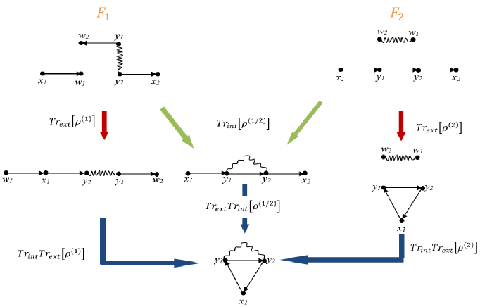
Figure 1: Scheme of partial traces over the possible quantum operator of the electron propagator at first order in $e$.

In the first case of eq.(15), in terms of Feynman diagrams, a positron and a photon field interact at the same space-time point and an electron in a different point. In the second case, an electron and a positron interact at the same space-time point and a photon field acts in a different space-time point. Both functions of the fields will contain the same reduced state when the internal degrees of freedom are traced out. Then, inserting eq.(14) in eq.(12) we obtain

$$iZ_{F}\left[\eta,\overline{\eta}\right]=\underset{n=0}{\overset{\infty}{\sum}}\underset{p=0}{\overset{\infty}{\sum}}\frac{i^{n}}{n!}\frac{i^{p}}{p!}\int\left\langle\Omega_{0}\left|T\psi(x_{1})\overline{\psi}(x_{2})...\psi(x_{n-1})\overline{\psi}(x_{n})\mathbf{F}(y_{1},..,y_{p},w_{1},...,w_{p})\right|\Omega_{0}\right\rangle$$ (16)

$$\eta(x_{1})\overline{\eta}(x_{2})...\eta(x_{n-1})\overline{\eta}(x_{n})\underset{i=1}{\overset{p}{\prod}}\delta(y_{i}-w_{i})\underset{i=1}{\overset{n}{\prod}}d^{4}x_{i}\underset{i=1}{\overset{p}{\prod}}d^{4}y_{i}d^{4}w_{i}$$

Now we can define two quantum operators in the following way

$$\varrho^{(F,n,p)}=\int\left\langle\Omega_{0}\left|T\psi(x_{1})\overline{\psi}(x_{2})...\psi(x_{n-1})\overline{\psi}(x_{n})\mathbf{F}(y_{1},..,y_{p},w_{1},...,w_{p})\right|\Omega_{0}\right\rangle$$ (17)

$$\left|x_{1},...,x_{\frac{n}{2}},y_{1},...,y_{p}\right\rangle\left\langle x_{\frac{n}{2}+1},...,x_{n},w_{1},...,w_{p}\right|\underset{i=1}{\overset{n}{\prod}}d^{4}x_{i}\underset{i=1}{\overset{p}{\prod}}d^{4}y_{i}d^{4}w_{i}$$

$$O^{(n,p)}=\int\eta(x_{1})\overline{\eta}(x_{2})...\eta(x_{n-1})\overline{\eta}(x_{n})\underset{i=1}{\overset{p}{\prod}}\delta(y_{i}-w_{i})\left|x_{1},...,x_{\frac{n}{2}},y_{1},...,y_{p}\right\rangle\left\langle x_{\frac{n}{2}+1},...,x_{n},w_{1},...,w_{p}\right|$$ (18)

$$\underset{i=1}{\overset{n}{\prod}}d^{4}x_{i}\underset{i=1}{\overset{p}{\prod}}d^{4}y_{i}d^{4}w_{i}$$

Then, eq.(16) can be written as

$$iZ_{F}\left[\eta,\overline{\eta}\right]=\underset{n=0}{\overset{\infty}{\sum}}\underset{p=0}{\overset{\infty}{\sum}}\frac{i^{n}}{n!}\frac{i^{p}}{p!}Tr(\varrho^{(F,n,p)}O^{(n,p)})$$ (19)

The quantum operator of eq.(18) has the following form

$$O^{(n,p)}=O_{ext}^{(n)}\otimes I_{int}^{(p)}$$ (20)

where

$$O_{ext}^{(n)}=\int\eta(x_{1})\overline{\eta}(x_{2})...\eta(x_{n-1})\overline{\eta}(x_{n})\left|x_{1},...,x_{\frac{n}{2}}\right\rangle\left\langle x_{\frac{n}{2}+1},...,x_{n}\right|\underset{i=1}{\overset{n}{\prod}}d^{4}x_{i}$$ (21)

and

$$I_{int}^{(p)}=\int\underset{i=1}{\overset{p}{\prod}}\delta(y_{i}-w_{i})\left|y_{1},...,y_{p}\right\rangle\left\langle w_{1},...,w_{p}\right|\underset{i=1}{\overset{p}{\prod}}d^{4}y_{i}d^{4}w_{i}=$$ (22)

$$\int\left|y_{1},...,y_{p}\right\rangle\left\langle y_{1},...,y_{p}\right|\underset{i=1}{\overset{p}{\prod}}d^{4}y_{i}$$

is an identity operator acting on the $y_{i}$ vertices that appear in the perturbation expansion. The Dirac delta that appears as the coefficient of the identity operator can be considered as a particular choice of an operator that physically implies no measurement. The subscript $ext$ in eq.(20) refers to the external points $x_{i}$ and the subscript $int$ to the internal vertices $y_{i}$. Then, the generating functional of eq.(12) can be written as the inner product of the quantum operator $O_{ext}$ on the reduced operator $\overline{\varrho}_{ext}$ as

$$Tr(\varrho^{(F,n,p)}O^{(n,p)})=Tr(\overline{\varrho}_{ext}^{(F,n,p)}O_{ext}^{(n)})$$ (23)

where

$$\overline{\varrho}_{ext}^{(F,n,p)}=Tr_{int}(\varrho^{(F,n,p)})=\int\left\langle y_{1},...,y_{p}\right|\varrho^{(F;n,p)}\left|y_{1},...,y_{p}\right\rangle\underset{i=1}{\overset{p}{\prod}}d^{4}y_{i}=$$ (24)

$$\int\left(\int\limits\left\langle\Omega_{0}\left|T\psi(x_{1})\overline{\psi}(x_{2})...\psi(x_{n-1})\overline{\psi}(x_{n})L_{I}^{0}(y_{1})...L_{I}^{0}(y_{p})\right|\Omega_{0}\right\rangle\underset{i=1}{\overset{p}{\prod}}d^{4}y_{i}\right)\times$$

$$\left|x_{1},...,x_{\frac{n}{2}}\right\rangle\left\langle x_{\frac{n}{2}+1},...,x_{n}\right|\underset{i=1}{\overset{n}{\prod}}d^{4}x_{i}$$

The procedure introduced above is suitable to consider the von Neumann entropy defined as $S_{ext/int}=-Tr\left[\varrho_{ext/int}\ln(\varrho_{ext/int})\right]$, where $\varrho_{ext/int}$ are partial traces with respect the internal/external vertices respectively. In $\phi^{4}$ theory, in the propagator, the contributions to the physical mass are given by the loop diagrams obtained from the perturbation theory. By ”opening” the loops, a quantum density operator can be defined, that represents the propagation of a defined number of entangled bosons. By considering the internal trace over this quantum operator, the boson propagator is recovered, represented by a reduced operator. In this sense, the dressed propagator of the boson is a reduced operator that represents a real propagating particle entangled with its virtual excitations and a measure of this entanglement is related to the physical mass, which is a consequence of the irrelevant degrees of freedom traced out. In the same way as for the $\phi^{4}$ theory, we can write the non-renormalized quantum state of the two-point correlation function that represents the electron propagation as

$$\rho_{ext}=\int\frac{d^{4}p}{(2\pi)^{4}}\frac{i}{p^{2}-m_{0}^{2}-\Sigma(p,m_{0}^{2})}\left|p\right\rangle\left\langle p\right|$$ (25)

where $\Sigma(p,m_{0}^{2})$ is the self-energy. For the sake of simplicity, the first contribution to $\Sigma$ comes from the diagram

$$\Sigma\sim\lambda_{0}\Delta_{0}+O(\lambda_{0}^{2})\sim\lambda_{0}\int d^{4}w_{1}\Delta(y_{1}-w_{1})\delta(y_{1}-w_{1})+O(\lambda_{0}^{2})$$ (26)

Because we can conceive the propagators as quantum density operators, then it is natural to interpret the coefficients of the operator as the probability amplitude attached to a particle travelling from one point $x_{1}$ to another point $x_{2}$ with an specific value of energy and momentum that a particle is created at $x_{1}$ and annihilated at $x_{2}$. Finally, it should be possible to apply the concept of entanglement entropy between real and virtual excitations for other systems that are treated perturbatively, for example for the Gell-Mann and Goldberger relation [45], in disordered systems in condensed matter [46] and whenever there is a generating functional for the correlation function or a generating function for the Green functions, as it is occur in condensed matter with the Luttinger-Ward functional [47].

3 The quantum entropy

In order to compute the quantum entropy we must take into account the algebraic structure of the Hilbert space involved in the procedure introduced in the previous section. The main difference between spinor quantum electrodynamics and $\phi^{4}$ theory is that in the latter, the coefficients of the quantum operators are complex numbers and in the first theory are $d\times d$ matrices due to the Dirac matrices in $d$ dimensions, where $d$ is the dimension of space-time when the dimensional regularization is applied. Nevertheless, the orders of the perturbation considered in this manuscript implies quantum operators where the $d\times d$ matrices are identity matrices, then the quantum operators can be written as

$$\varrho^{(n)}=[Tr(\varrho^{(n)})]^{-1}\left[\varrho^{(n,0)}\oplus\varrho^{(n,1)}\oplus...\oplus\varrho^{(n,i)}...\right]=[Tr(\varrho^{(n)})]^{-1}\underset{j=0}{\overset{+\infty}{\oplus}}\varrho^{(n,i)}$$ (27)

where the superscript $n~{}$indicates the number of external points and $i$ indicates the order in the perturbation expansion. $[Tr(\varrho^{(n)})]^{-1}$ is the normalization of the quantum operator that can be introduced at the right or left of $\underset{j=0}{\overset{+\infty}{\oplus}}\varrho^{(n,i)}$ because is only a diagonal matrix. The coefficient of each quantum operator will be of the form

$$\varrho^{(n,i)}(x_{1},...,x_{n},y_{1},...,y_{p},w_{1},...,w_{p})=$$ (28)

$$\left\langle\Omega_{0}\left|T\psi(x_{1})\overline{\psi}(x_{2})...\psi(x_{n-1})\overline{\psi}(x_{n})F(y_{1},..,y_{p},w_{1},...,w_{p})\right|\Omega_{0}\right\rangle$$

The trace reads

$$Tr(\varrho^{(n)})=\underset{j=0}{\overset{+\infty}{\sum}}(-e)^{j}W_{(n,j)}Tr(\rho^{(n,j)})$$ (29)

where $W_{(n,i)}$ is the weight factor (see [48]) corresponding to the connected Feynman diagram and $\rho^{(n,j)}$ is an operator that depends on the propagator of the respective Feynman diagram. The total quantum entropy can be computed as

$$S^{(n)}=-Tr[\varrho^{(n)}\ln(\varrho^{(n)})]$$ (30)

where $S$ will be a function of $e$ and some factor which will depend on the regularization scheme chosen. Up to second order in $e$, the quantum entropy in terms of $\rho$ reads

$$S^{(n)}=\ln(\beta^{(n,0)})-[\beta^{(n,0)}]^{-1}Tr[\rho^{(n,0)}\ln(\rho^{(n,0)})]$$ (31)

$$-\frac{e^{2}W_{(n,1)}}{W_{(n,0)}[\beta^{(n,0)}]^{2}}\left[\beta^{(n,1)}Tr[\rho^{(n,0)}\ln(\rho^{(n,0)})]-\beta^{(n,0)}Tr[\rho^{(n,1)}\ln(\rho^{(n,0)})]\right]+O(\lambda_{0}^{2})$$

where $\beta^{(n,i)}=Tr(\rho^{(n,i)})$.

3.1 Free fermion field entropy

In the case of two external points, at zero order in $e$, $\beta^{(2,0)}=Tr[\rho_{ext}^{(2,0)}]$ and $Tr[\rho_{ext}^{(2,0)}\ln(\rho_{ext}^{(2,0)})]$ must be computed. The quantum operator at zero order is the free propagator

$$\rho_{ext_{F}}^{(2,0)}=\int\frac{d^{4}p}{(2\pi)^{4}}\frac{i(\not{p}+m_{0})e^{-ip(x_{1}-x_{2})}}{p^{2}-m_{0}^{2}}\left|x_{1}\right\rangle\left\langle x_{2}\right|d^{4}x_{1}d^{4}x_{2}$$ (32)

Taking the Fourier transform by writing $\left|x_{1}\right\rangle=\int\frac{d^{4}q_{1}}{(2\pi)^{4}}e^{-iq_{1}x_{1}}\left|q_{1}\right\rangle$ and $\left\langle x_{2}\right|=\int\frac{d^{4}q_{2}}{(2\pi)^{4}}e^{iq_{2}x_{2}}\left\langle q_{2}\right|$, performing a Wick rotation $p_{0E}=-ip_{0}$, $p_{iE}=p_{i}$, $d^{4}p=id^{4}p_{E}$ the quantum operator $\rho_{ext}^{(2,0)}$ in momentum space is diagonal and reads

$$\rho_{ext_{F}}^{(2,0)}=\int\frac{d^{4}p_{E}}{(2\pi)^{4}}\frac{(\not{p}_{E}+m_{0})}{p_{E}^{2}+m_{0}^{2}}\left|p_{E}\right\rangle\left\langle p_{E}\right|$$ (33)

where $\not{p}_{E}=\gamma_{E}^{\mu}p_{\mu_{E}}$, and $\gamma_{E}^{\mu}$ are the Euclidean Dirac matrices $\gamma_{E}^{0}=\gamma^{0}$, $\gamma_{E}^{i}=-i\gamma^{i}$. The trace of $\rho_{ext_{F}}^{(2,0)}$ reads $\beta_{F}^{(2,0)}=Tr[\rho_{ext_{F}}^{(2,0)}]=2TVm_{0}\Delta_{0}$, where

$$\Delta_{j}=\int\frac{d^{4}p_{E}}{(2\pi)^{4}}\frac{1}{(p_{E}^{2}+m_{0}^{2})^{j+1}}$$ (34)

where the integral of the term with odd $p_{\mu_{E}}$ in the numerator vanishes by symmetry and where $2TV=\int d^{4}x=\delta^{(4)}(0)$ (see [48], page 96). It is interesting to note that $\beta_{F}^{(2,0)}$ for fermions is different from scalar boson fields, where $\beta_{B}^{(2,0)}=Tr[\rho_{ext_{B}}^{(2,0)}]=2TV\Delta_{0}$ (see eq.(32) of [25]). Because $\rho^{(2,0)}$ is diagonal in the momentum basis, $\ln[\rho_{ext_{F}}^{(2,0)}]$ reads

$$\ln[\rho_{ext_{F}}^{(2,0)}]=\int\frac{d^{4}p_{E}}{(2\pi)^{4}}\ln(\frac{\not{p}_{E}+m_{0}}{p_{E}^{2}+m_{0}^{2}})\left|p_{E}\right\rangle\left\langle p_{E}\right|$$ (35)

By computing the matrix logarithm of $\frac{\not{p}_{E}+m_{0}}{p_{E}^{2}+m_{0}^{2}}$ we obtain (see eq.(77) of Appendix B)

$$\ln(\frac{\not{p}_{E}+m_{0}}{p_{E}^{2}+m_{0}^{2}})=-\frac{1}{2}\ln(p_{E}^{2}+m_{0}^{2})I+\frac{\not{p}_{E}}{2p_{E}}\ln(\frac{m_{0}+p_{E}}{m_{0}-p_{E}})$$ (36)

Then, by multiplying eq.(35) with $\rho_{ext}^{(2,0)}$ we obtain

$$\rho_{ext_{F}}^{(2,0)}\ln[\rho_{ext_{F}}^{(2,0)}]=\int\frac{d^{4}p_{E}}{(2\pi)^{4}}\frac{\not{p}_{E}+m_{0}}{p_{E}^{2}+m_{0}^{2}}\ln(\frac{\not{p}_{E}+m_{0}}{p_{E}^{2}+m_{0}^{2}})\left|p_{E}\right\rangle\left\langle p_{E}\right|$$ (37)

Then the trace $Tr[\rho_{ext_{F}}^{(2,0)}\ln(\rho_{ext_{F}}^{(2,0)})]$ reads

$$Tr[\rho_{ext_{F}}^{(2,0)}\ln(\rho_{ext_{F}}^{(2,0)})]=TV\left[\eta_{0}-m_{0}\chi_{0}\right]$$ (38)

where $\eta_{0}$ reads

$$\eta_{0}=\int\frac{d^{4}p_{E}}{(2\pi)^{4}}\frac{p_{E}}{p_{E}^{2}+m_{0}^{2}}\ln(\frac{m_{0}+p_{E}}{m_{0}-p_{E}})$$ (39)

and

$$\chi_{0}=\int\frac{d^{4}p_{E}}{(2\pi)^{4}}\frac{\ln(p_{E}^{2}+m_{0}^{2})}{p_{E}^{2}+m_{0}^{2}}$$ (40)

which has been computed in [25], eq.(36) and eq.(A3) of Appendix B). In eq.(38) we have disregarded the odd term in $\not{p}_{E}$ because it integrates symmetrically to zero. Taking into account all the terms and using eq.(31) at zero order, the quantum entropy of the free electron propagation reads

$$S_{ext_{F}}^{(2)}=\ln(2TVm_{0}\Delta_{0})-\frac{\eta_{0}}{2m_{0}\Delta_{0}}+\frac{\chi_{0}}{2\Delta_{0}}$$ (41)

where $\Delta_{0}$ was computed in [25] using dimensional regularization. Applying the same regularization scheme in $\eta_{0}$ and $\chi_{0}$, the external entropy at zero order in the perturbation expansion reads

$$S_{ext_{F}}^{(2)}=-\frac{1}{\epsilon}-\frac{11}{6}+\ln(\frac{m_{0}^{4}TV}{4\pi^{2}\epsilon})+O(\epsilon)$$ (42)

where $\epsilon=d-4$ can be considered as a microscopic cutoff. The appearance of the logarithm of the microscopic cutoff $\epsilon$ has been obtained in other works [49], [50], [51], [52] and [53]. The entropy is proportional to the dimensionless coefficient $\frac{m_{0}^{4}TV}{4\pi^{2}}$ similar to the result obtained in [25] for the scalar boson which is $S_{ext_{B}}^{(2)}=\ln(2TV\Delta_{0})+\frac{\chi_{0}}{\Delta_{0}}=-\frac{2}{\epsilon}-1+\ln(\frac{m_{0}^{4}TV}{4\pi^{2}\epsilon})+O(\epsilon)$, where $\Delta_{0}$ and $\chi_{0}$ are defined in eq.(34) and eq.(40). By comparing with eq.(42) for the particular case of identical masses for the fermion and boson excitations we obtain

$$S_{ext_{F}}^{(2)}-S_{ext_{B}}^{(2)}=-\frac{1}{\epsilon}-\frac{5}{6}+O(\epsilon)$$

By negleting the $1/\epsilon$ divergent term, $S_{ext_{B}}^{(2)}=\frac{5}{6}+S_{ext_{F}}^{(2)}$ the boson field entropy is larger than the fermion field entropy of propagation in the space-time for identical masses.

3.2 Free photon field entropy

In the case of an external photon propagating, the two external points, at zero order in $e$ reads

$$\rho_{ext_{P}}^{(2,0)}=I_{\mu_{1}\mu_{2}}\int\frac{d^{4}p_{E}}{(2\pi)^{4}}\frac{1}{p_{E}^{2}+m_{\gamma}^{2}}\left|p_{E}\right\rangle\left\langle p_{E}\right|$$ (43)

where $m_{\gamma}$ is ficticious photon mass to avoid infrared divergences. The trace reads

$$Tr(\rho_{\mu\nu}^{(2,0)})=I_{\mu_{1}\mu_{2}}2TV\int\frac{d^{d}\mathbf{p}_{E}}{(2\pi)^{d}}\frac{1}{p_{E}^{2}+m_{\gamma}^{2}}=I_{\mu_{1}\mu_{2}}2TV\Delta_{0}(m_{\gamma})$$ (44)

The quantum entropy of free photons reads

$$S_{ext_{P}}^{(2,0)}=\ln(2TV\Delta_{0}(m_{\gamma}))+\frac{\chi_{0}(m_{\gamma})}{\Delta_{0}(m_{\gamma})}$$ (45)

The result obtained is identical to the quantum entropy of a free scalar boson but with $m_{0}$ replaced by $m_{\gamma}$ and the limit $m_{\gamma}\rightarrow 0$ must be taken. From last equation an infrared divergence appears. Nevertheless, it is well known from the theorem due to Kinoshita-Lee and Nauenberg ( [30] and [31]) that any physically observable must be infrared safe. To avoid the fictitious mass $m_{\gamma}$, a sum over additional photon emissions must be computed. This point is very important, because in order to obtain finite values of the observables in the infrared limit, we must consider that in the scattering process there are some soft photons unobserved. In [25] a mathematical structure for this unobserved propagation was introduced. In fact, the perturbation expansion of any quantum field theory allows rewriting the different contributions as partial traces over some degrees of freedom that represent particles that are not detected. In several texts, the discussion is introduced in the context of the vertex correction to the electron propagator. The first virtual contribution comes from a photon connecting two electron propagator. To this virtual contribution we must add the real soft photon contribution, that is nothing more than ”opening” the virtual photon propagator (see page 199 and page 203 of [48]). Is interesting to note that we can avoid infrared divergences by considering that unobserved photons are contributing. In [25] a discussion about $\phi^{4}$ theory implies that the first contribution to the scalar boson propagator implies not measuring a third scalar propagator. This unobserved boson implies tracing over its degrees of freedom and this corresponds to ”close” the propagator and obtain the loop, which introduces an ultraviolet divergence. Following the same procedure, it is possible to introduce soft photon emissions in the quantum entropy by simply adding to eq.(43) a quantum state with ficticious mass $m_{\gamma}$ but that is integrated in momentum from $0$ to $E_{c}\,$, where $E_{c}$ is the maximum photon energy allowed to escape detection. Computing the eq.(45) and considering the $d\rightarrow 4$ limit, the quantum entropy of a free photonic field reads

$$S_{ext_{P}}^{(2,0)}=-\frac{2}{\epsilon}-1+\ln(\frac{E_{c}^{4}TV}{4\pi^{2}\epsilon})+O(\epsilon)$$ (46)

The logarithmic behavior is identical to the free bosonic and fermionic quantum entropies and is an universal feature of the entanglement entropy for free quantum fields. It diverges with the cutoff as $\epsilon^{-1}$ and $\ln(\epsilon)$ and the finite part depends on some complex number and the logarithm of some dimensionless number $m_{0}^{4}TV$.

3.3 First correction to the fermion field entropy

In this case the total quantum operator at second order in $e$ for the electron propagator reads

$$\rho_{ext_{F}}^{(2,1)}=\int\frac{d^{d}p}{(2\pi)^{d}}\frac{d^{d}q}{(2\pi)^{d}}\frac{i(\not{p}+m_{0})e^{-i\mathbf{p}\cdot\mathbf{x}_{1}}}{p^{2}-m_{0}^{2}}\gamma^{\mu_{1}}\frac{i(\not{q}+m_{0})}{q^{2}-m_{0}^{2}}\gamma^{\mu_{2}}\frac{i(\not{p}+m_{0})e^{i\mathbf{p}\cdot\mathbf{x}_{2}}}{p^{2}-m_{0}^{2}}\frac{-ig_{\mu_{1}\mu_{2}}}{(p-q)^{2}}\left|x_{1}\right\rangle\left\langle x_{2}\right|$$ (47)

$$d^{4}y_{1}d^{4}y_{2}d^{4}x_{1}d^{4}x_{2}$$

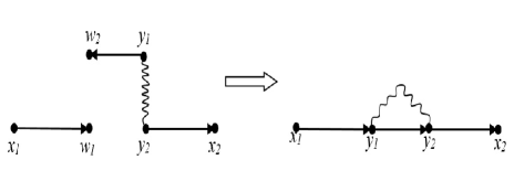
Figure 2: Left: open Feynmann diagram representing the quantum operator at second order in $e$ for the fermion propagator. Right: Partial trace over the internal degrees of freedom $y_{1}$, $w_{1}$, $y_{2}$ and $w_{2}$ which gives the self-energy contribution to the electron propagator.

This quantum state can be obtained by computing the trace over the internal degrees of freedom represented by the basis $\left|y_{1},y_{2}\right\rangle\left\langle w_{1},w_{2}\right|$ over the quantum operator defined as (see figure 2)

$$\rho_{F}^{(2,1)}=\int S_{F}(x_{1}-y_{1})\gamma^{\mu_{1}}S_{F}(y_{2}-w_{1})\gamma^{\mu_{2}}S_{F}(w_{2}-x_{2})D_{P}(y_{1}-y_{2})g_{\mu_{1}\mu_{2}}\left|x_{1},y_{1},y_{2}\right\rangle\left\langle x_{2},w_{1},w_{2}\right|$$ (48)

$$d^{d}x_{1}d^{d}x_{2}d^{d}y_{1}d^{d}w_{1}d^{d}y_{2}d^{d}w_{2}$$

where $S_{F}$ is the fermionic propagtor and $D_{P}$ is the photon propagator. By applying Wick rotation and computing the Fourier transform, the quantum operator reads

$$Tr_{int}[\rho_{F}^{(2,1)}]=\rho_{ext_{F}}^{(2,1)}=$$ (49)

$$=-\int\frac{d^{d}p_{E}}{(2\pi)^{d}}\frac{(\not{p}_{E}+m_{0})}{p_{E}^{2}+m_{0}^{2}}\Sigma_{2}(\not{p}_{E})\frac{(\not{p}_{E}+m_{0})}{p_{E}^{2}+m_{0}^{2}}\left|p_{E}\right\rangle\left\langle p_{E}\right|$$

where $\Sigma_{2}(\not{p}_{E})$ is the second order in $e$ contribution to the self-energy (see eq.(7.16) of [48]). From eq.(10.41) of [48], $\Sigma_{2}$ can be written as $\Sigma_{2}(\not{p}_{E})=\Sigma_{2}^{(0)}(p_{E})-\Sigma_{2}^{(1)}(p_{E})\not{p}_{E}$, where

$$\Sigma_{2}^{(0)}(p_{E}) = \frac{e^{2}}{(4\pi)^{d/2}}\int_{0}^{1}dx\frac{\Gamma(2-\frac{d}{2})(4-\epsilon)m_{0}}{[(1-x)m_{0}^{2}+x\mu^{2}-x(1-x)p_{E}^{2}]^{2-\frac{d}{2}}}$$ (50)

$$\Sigma_{2}^{(1)}(p_{E}) = \frac{e^{2}}{(4\pi)^{d/2}}\int_{0}^{1}dx\frac{\Gamma(2-\frac{d}{2})(2-\epsilon)x}{[(1-x)m_{0}^{2}+x\mu^{2}-x(1-x)p_{E}^{2}]^{2-\frac{d}{2}}}$$

We can write $(\not{p}_{E}+m_{0})\Sigma_{2}(\not{p}_{E})(\not{p}_{E}+m_{0})=A_{0}(p_{E})+A_{1}(p_{E})\not{p}_{E}$, where

$$A_{0}(p_{E}) = \Sigma_{2}^{(0)}\left(p_{E}^{2}+m_{0}^{2}\right)-2m_{0}\Sigma_{2}^{(1)}p_{E}^{2}$$ (51)

$$A_{1}(p_{E}) = m_{0}\Sigma_{2}^{(0)}-\Sigma_{2}^{(1)}\left(m_{0}p_{E}^{2}+m_{0}^{2}\right)$$

In order to compute $Tr[\rho_{ext_{F}}^{(2,1)}\ln(\rho_{ext_{F}}^{(2,0)})]$, we note that the $\ln(\rho_{ext_{F}}^{(2,0)})$ has been computed in eq.(36), so that

$$Tr[\rho_{ext_{F}}^{(2,1)}\ln(\rho_{ext_{F}}^{(2,0)})]=-2TV\int\frac{d^{d}p_{E}}{(2\pi)^{d}}\frac{A_{0}(p_{E})\ln(p_{E}^{2}+m_{0}^{2})}{2(p_{E}^{2}+m_{0}^{2})^{2}}$$ (52)

$$-2TV\int\frac{d^{d}p_{E}}{(2\pi)^{d}}\frac{A_{1}(p_{E})p_{E}}{2(p_{E}^{2}+m_{0}^{2})^{2}}\ln(\frac{m_{0}+p_{E}}{m_{0}-p_{E}})$$

where we have neglected the odd terms in $\not{p}_{E}$ because they integrate symmetrically to zero. In turn, the trace of $\rho_{ext_{F}}^{(2,1)}$ reads

$$\beta^{(2,1)}=-2TV\int\frac{d^{d}p_{E}}{(2\pi)^{d}}\frac{A_{0}(p_{E})}{(p_{E}^{2}+m_{0}^{2})^{2}}$$ (53)

Eqs.(53) and (52) are complicated integrals that give the second order contribution to the fermion entropy. Instead of computing the last integrals, we can consider a more simple system in which the full propagator can be solved exactly. This model is the Bloch-Nordsieck model [42], where the Dirac matrices $\gamma^{\mu}$ in the Lagrangian are replaced by $u^{\mu}$, where $u^{\mu}$ are the components of a velocity vector and $u^{\mu}u_{\mu}=1$. This model has been solved in [54] and an exact solution to the full Green function reads (see [55], eq.(46.28), page 484)

$$G(p)=\frac{1}{(u_{\mu}p^{\mu}-m_{0})^{\gamma+1}}$$ (54)

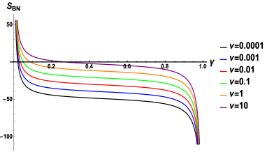
Figure 3: Right: Total entropy as a function of $\gamma$ for different values of the ratio $\nu=\frac{m_{0}^{4}TV}{\cos^{4}\theta}$ for the Bloch-Nordsieck model. Left: Difference between total entropy and entropy without interactions for the Bloch-Nordsieck model as a function of $\gamma=\frac{\alpha}{2\pi}(3-\xi)$.

where $\gamma=\frac{e^{2}}{8\pi^{2}}(3-\xi)=\frac{\alpha}{2\pi}(3-\xi)$, where $\alpha$ is the fine structure constant and $\xi$ is a gauge fixing parameter. We can write $u_{\mu}p^{\mu}=\left|p\right|\cos\theta$, where $\theta$ is the angle between $u$ and $p$. This full propagator is the analogue to the full propagator of a $\phi^{4}$ theory written in terms of the partial trace of a quantum density operator (see [27], eq.(65)) or the full electron propagator of QED, $G=(p^{2}-m_{0}^{2}-\Sigma(\not{p}))^{-1}$. As we write the quantum operator for the electron or boson propagator, we can do the same with the quantum state in the Bloch-Nordsieck model as

$$\rho=\int\frac{d^{4}p}{(2\pi)^{4}}\frac{1}{(p\cos\theta-m_{0})^{\gamma+1}}\left|p\right\rangle\left\langle p\right|$$ (55)

The quantum entropy can be computed as $S_{BN}=\ln\left[2TV\Delta\right]+\frac{(\gamma+1)}{\Delta}\Gamma$, where

$$\Delta=\frac{1}{8\pi^{2}}\int_{0}^{\infty}\frac{p^{3}}{(p\cos\theta-m_{0})^{\gamma+1}}dp=\frac{6(-1)^{3-\gamma}(m_{0})^{3-\gamma}}{8\pi^{2}(\gamma-3)(\gamma-2)(\gamma-1)\gamma\cos^{4}\theta}$$ (56)

and

$$\Gamma=\frac{1}{8\pi^{2}}\int\frac{p^{3}\ln(up-m_{0})}{(up-m_{0})^{\gamma+1}}dp=$$ (57)

$$\frac{6(-1)^{\gamma}(m_{0})^{\gamma}m_{0}^{3}[-2(2\gamma-3)(1+\gamma(\gamma-3))-(\gamma-3)(\gamma-2)\gamma\ln(-m_{0})]}{8\pi^{2}(\gamma-3)^{2}(\gamma-2)^{2}(\gamma-1)^{2}\gamma^{2}\cos^{4}\theta}$$

Then

$$S_{BN}=\frac{1+\gamma}{\gamma}+\frac{1+\gamma}{\gamma-1}+\frac{1+\gamma}{\gamma-2}+\frac{1+\gamma}{\gamma-3}+\ln[\frac{3m_{0}^{4}TV}{2\pi^{2}\cos^{4}\theta(\gamma-3)(\gamma-2)(\gamma-1)\gamma}]$$ (58)

By considering the limit $\gamma\rightarrow 0$, $\Delta S_{BN}=S_{BN}(\gamma)-S_{BN}(0)$ reads

$$\Delta S_{BN}=\frac{11}{6}+\frac{1+\gamma}{\gamma-1}+\frac{1+\gamma}{\gamma-2}+\frac{1+\gamma}{\gamma-3}+\ln[\frac{6}{(3-\gamma)(2-\gamma)(1-\gamma)}]$$ (59)

In figure 3 the total entropy for different values of $\frac{m_{0}^{4}TV}{\cos^{4}\theta}$ is shown in the first case and the difference of the total entropy with respect the non-interacting case $\Delta S_{BN}$ is shown as a function of $\gamma$ in the second case. As it can be seen, the interactions decrease the fermion entropy. In fact, by replacing $\gamma$ by $\frac{\alpha}{\pi}$, where the Feynman gauge is considered $\xi=1$, we obtain $\Delta S_{BN}\sim-0.003$, which is the entropy lost by the interactions. This is the same behaviour found in the quantum entropy of the boson field. In [25], it was shown that the quantum entropy at first order in $\lambda_{0}$ for the boson field reads

$$S_{B}^{ext}=\ln(2TV\Delta_{0})+\frac{\chi_{0}}{\Delta_{0}}+\frac{\lambda_{0}\mu^{-\epsilon}}{2}\left(\chi_{1}-\frac{\Delta_{1}\chi_{0}}{\Delta_{0}}\right)+O(\lambda_{0}^{2})$$ (60)

$$=-\frac{2}{\epsilon}-1+\ln(\frac{m_{0}^{4}TV}{4\pi^{2}\epsilon})+\frac{\lambda_{0}}{32\pi^{2}}\left(-1+2\gamma_{0}+\ln(\frac{m_{0}^{4}}{4\pi^{2}\mu^{4}})\right)+O(\lambda_{0}^{2})$$

where $\gamma_{0}$ is the Euler-Mascheroni constant. The contribution at order $\lambda_{0}$ is similar to the results obtained in [26] for the mutual information. In figure 4, the total entropy is plotted as a function of $\frac{m_{0}}{\mu}$, where it can be seen that the contribution at first order in $\lambda_{0}$ decreases the quantum entropy with respect the free value. This result for the Bloch-Nordsieck and the scalar boson suggests that interactions reduce the unpredictability of the quantum operator propagation.

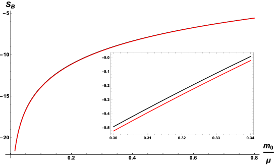
Figure 4: Quantum entropy of boson propagator at zero order in $\lambda_{0}$ (black line) and at first order in $\lambda_{0}$ (red line).

On the other hand, by computing the integrals of eq.(56) and eq.(57) in $d$ dimensions, taking the limit $d\rightarrow 4$ and finally the $\gamma\rightarrow 0$ limit, the quantum entropy can be written as

$$S_{BN}=-\frac{1}{\epsilon}-\frac{11}{6}+\ln(\frac{m_{0}^{4}TV}{4\pi^{2}\epsilon\cos^{4}\theta})-\frac{49}{36}\gamma-\frac{199}{108}\gamma^{2}-O(\gamma^{3})$$ (61)

where the finite term $-\frac{11}{6}$ is identical to the QED interaction (see eq.(42)). Without loss of generality, taking $\cos\theta=1$, then the free quantum entropy obtained follows the same behavior as the quantum entropy for free fermions (see eq.(42). The logarithm term $\ln(\frac{m_{0}^{4}TV}{4\pi^{2}\epsilon})$ is universal for the different quantum fields.

3.4 First correction to the photon field entropy

The quantum operator of the first correction to the photon propagator reads (see figure 5)

$$\rho_{P}^{(2,1)}=\int D_{P}(x_{1}-y_{1})g_{\mu_{1}\rho}S_{F}(y_{1}-w_{2})\gamma^{\rho}\gamma^{\nu}S_{F}(w_{1}-y_{2})D_{P}(y_{2}-x_{2})g_{\nu\mu_{2}}\times$$ (62)

$$\left|x_{1},y_{1},y_{2}\right\rangle\left\langle x_{2},w_{1},w_{2}\right|d^{d}x_{1}d^{d}x_{2}d^{d}y_{1}d^{d}w_{1}d^{d}y_{2}d^{d}w_{2}$$

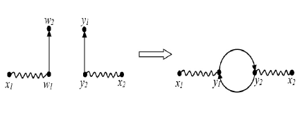
Figure 5: Left: open Feynmann diagram representing the quantum operator at second order in $e$ for the photon propagator. Right: Partial trace over the internal degrees of freedom $y_{1}$, $w_{1}$, $y_{2}$ and $w_{2}$ which gives the self-energy contribution to the photon propagator.

The partial trace over the internal degrees of freedom $y_{1}$, $\omega_{1}$ and $y_{2}$, $w_{2}$ gives as a result the first quantum correction to the photon propagator reads

$$\rho_{ext_{P}}^{(2,1)}=\int\frac{d^{d}p}{(2\pi)^{d}}\frac{\Pi_{2}^{\mu_{1}\mu_{2}}(p)}{(p^{2}+\mu^{2})^{2}}\left|p\right\rangle\left\langle p\right|$$ (63)

where we have used that introduced the Fourier transform of $\left|x_{1}\right\rangle$ and $\left\langle x_{2}\right|$ and where (see eq.(7.71) of [48])

$$\Pi_{2}^{\mu_{1}\mu_{2}}(p)=\int\frac{d^{d}q}{(2\pi)^{d}}tr\left[\gamma^{\mu_{1}}\frac{i}{\not{q}-m_{0}}\gamma^{\mu_{2}}\frac{i}{\not{q}+\not{p}-m_{0}}\right]$$ (64)

which in turn can be written as $\Pi_{2}^{\mu_{1}\mu_{2}}(p)=(p^{2}\delta_{\mu_{1}\mu_{2}}-p^{\mu_{1}}p^{\mu_{2}})\Pi_{2}(p)$, where

$$\Pi_{2}(p)=-\frac{8}{(4\pi)^{d/2}}\int_{0}^{1}dx\frac{x(1-x)\Gamma(2-\frac{d}{2})}{[m_{0}^{2}-x(1-x)p^{2}]^{2-\frac{d}{2}}}$$ (65)

The quantum entropy at second order in $e$ implies to compute two integrals

$$\beta^{(2,1)}=Tr[\rho_{ext_{P}}^{(2,1)}]=2TV\int\frac{d^{d}p}{(2\pi)^{d}}\frac{\Pi_{2}^{\mu_{1}\mu_{2}}(p)}{(p^{2}+\mu^{2})^{2}}$$ (66)

and

$$Tr[\rho_{ext_{P}}^{(2,1)}\ln(\rho_{ext_{P}}^{(2,1)})]=-2TV\int\frac{d^{d}p}{(2\pi)^{d}}\frac{\Pi_{2}^{\mu_{1}\mu_{2}}(p)\ln(p^{2}+\mu^{2})}{(p^{2}+\mu^{2})^{2}}$$ (67)

where we have disregarded terms with odd $p_{\mu_{E}}$ and $q_{\mu_{E}}$ in the numerator. Last integrals can be solved in order to obtain the first contribution to the quantum entropy of the photon propagation. Considering the Bloch-Nordsieck model, in contrast with the fermionic self-energy, there is no vacuum polarization, which is the effect of the photon self-energy. Then it is not possible to obtain other contributions to the quantum entropy in this model than the result obtained in eq.(46).

Summing up, we can collect all the results for the free quantum entropies for different quantum fields

$$S_{B}=-\frac{2}{\epsilon}-1+\ln(\frac{m_{B}^{4}TV}{4\pi^{2}\epsilon})$$ (68)

$$S_{F}=-\frac{1}{\epsilon}-\frac{11}{6}+\ln(\frac{m_{F}^{4}TV}{4\pi^{2}\epsilon})$$

$$S_{P}=-\frac{2}{\epsilon}-1+\ln(\frac{E_{c}^{4}TV}{4\pi^{2}\epsilon})$$

which can be condensed in

$$S_{i}=-\frac{a_{i}}{\epsilon}-b_{i}+\ln(\frac{m_{i}^{4}TV}{4\pi^{2}\epsilon})$$ (69)

where we can consider that the maximum photon energy allowed to escape detection $E_{l}$ can be considered as an of-shell photon mass. For any two scalar bosons with different masses $m_{B_{1}}$ and $m_{B_{2}}$we have that $S_{B_{1}}-S_{B_{2}}=4\ln(\frac{m_{B_{1}}}{m_{B_{2}}})$. In turn, $S_{B}-S_{F}=\frac{5}{6}+4\ln(\frac{m_{B}}{m_{F}})$ and if $m_{B}>e^{-\frac{5}{24}}m_{F}$ then $S_{B}>S_{F}$. The different quantum entropies contain ultraviolet divergences which can be isolated by dimensional regularization. It should be stressed that even in the most simple case where no interactions are considered, the von Neumann entropy contains ultraviolet divergences (see eq.(68)). This implies that no mathematical operation at the level of the density quantum operators exists to avoid UV divergences. The von Neumann entropy for the free scalar propagator depends only on the mass of the quantum field $m_{0}$, the space-time volume and the ultraviolet cutoff. These divergences appear similarly in the entanglement entropy between regions of space-time [9]. In local quantum field theory, discussions of entanglement are focused on the density matrices associated with bounded spatial regions. These results are well-defined because by locality, there are independent degrees of freedom in disjoint spatial domains, so the Hilbert space factorizes. The associated spatial entanglement entropy is typically divergent, even in free field theory, because in the continuum limit, any spatial region contains an infinite number of degrees of freedom produced by high energy vacuum fluctuations at arbitrarily short wavelengths. These divergences require regularization and some procedure is needed to extract finite regularization independent data.

In entanglement entropy between space-time regions, the terms that are proportional to $\frac{1}{\epsilon^{j}}$ are not physical since they are not related to quantities well defined in the continuum ([9]). The logarithmic divergence is expected to be universal in the sense that is independent of the regularization prescription adopted or of the microscopic model used to obtain the continuum QFT at distances large with respect to the cutoff.

4 Conclusions

In this work, the entanglement entropy between real and virtual propagating states has been computed by rewriting the generating functional of the quantum electrodynamics theory in terms of quantum operators and inner products. In this way, it is possible to compute the von Neumann entropy for the electron and photon propagator as a perturbation expansion in $e$. It was shown that for the Bloch-Nordsieck model, the interactions decrease the quantum entropy with respect the non-interacting case. In turn, it is shown the universal behavior of the von Neumann entropy for different free quantum fields, that depends on the logarithm of the dimensionless parameter $\frac{m^{4}TV}{\epsilon}$ and some particular constants. The first order contributions to the entropy of the fermion and photon fields are considered and the results are computed in terms of complex integrals. The formalism introduced can be useful to characterize the entanglement entropy that interactions introduce. In turn, the entanglement can be understood as unobserved field excitations which are traced out.

5 Acknowledgment

This paper was partially supported by grants of CONICET (Argentina National Research Council) and Universidad Nacional del Sur (UNS) and by ANPCyT through PICT 1770, and PIP-CONICET Nos. 114-200901-00272 and 114-200901-00068 research grants. J. S. A. is member of CONICET.

Appendix A Appendix A

In order to get closer the ideas of this manuscript and the general boundary formalism only for boundaries defined by spacelike hyperplanes consider the quantum scalar field

$$\phi_{0}(x)=\int\frac{d^{3}p}{(2\pi)^{3}}\frac{1}{\sqrt{2E_{p}}}\left(\mathbf{a}_{p}e^{ipx}+\mathbf{a}_{p}^{{\dagger}}e^{-ipx}\right)$$ (70)

then consider this quantum field as the coordinate representation of a ket $\left|\phi_{0}(x_{1})\right\rangle$ in the space-time coordinate $x_{1}$ and another quantum field in the space-time coordinate $x_{2}$, that is $\left|\phi_{0}(x_{2})\right\rangle$, where the time component of $x_{1}$ is smaller than the time component of $x_{2}$ (see [35] below eq.(3)). If we suppose that the time-component of $x_{1}$ is smaller than the time component of $x_{2}$ and the space coordinates can vary over a space-like hyperplane, then we can define the quantum density operator

$$\rho_{0}=\left|\phi_{0}(x_{1})\right\rangle\left\langle\phi_{0}(x_{2})\right|$$ (71)

then is not difficult to show that

$$\left\langle\Omega_{0}\left|\rho_{0}\right|\Omega_{0}\right\rangle=\Delta_{0}(x_{1}-x_{2})$$ (72)

that is, the coefficient of the quantum operator of eq.(31) of [25] is the vacuum expectation value of the quantum density operator defined in eq.(71), that is $\rho=\int\left\langle\Omega_{0}\left|\rho_{0}\right|\Omega_{0}\right\rangle\left|x_{1}\right\rangle\left\langle x_{2}\right|d^{3}\mathbf{r}_{1}d^{3}\mathbf{r}_{2}$, where the time components of $x_{1}$ and $x_{2}$ are fixed and not integrated. This quantum operator is suitable for processes where a preparation is done in $t_{1}$ and a measurement is done in $t_{2}$ or more simpler a creation and a later annihilation of a field excitation. For virtual processes this quantum state is not suitable because the perturbation expansion demands that an integration $\int d^{4}y$ must be computed (is the superposition principle [48], p. 94).

For external points is not possible to restrict the quantum operator to a single time slice because the time component of $x_{1}$ must be smaller than the time component of $x_{2}$ and in turn $t_{1}$ and $t_{2}$ must be fixed. For virtual propagations there is no restriction and can be the case in which $t_{2}=t_{1}$, that is, the quantum operator is restricted to a single time-slice. The procedure done in [25] manifest this virtual process as a real propagator $\Delta(y_{1}-w_{1})$ between two arbitrary space-time coordinates $y_{1}$ and $w_{1}$ and a sum over all the possible space-time coordinates $y_{1}$ and $w_{1}$ must be done. This sum is provided by the lack of measurement of these two space-time points by introducing the Dirac delta distribution $\delta(y_{1}-w_{1})$ as the internal part of the observable. From this point of view, there is an identification of virtual propagation with real propagation by opening the loop $y_{1}\rightarrow y_{1}$ to $y_{1}\rightarrow w_{1}$. This happens only when interactions are turned on. Processes as propagation or scattering events happen inside a space-time region, which is the space-time region relevant for the experiment, in the sense that the particle inflow and detection happens on the boundary of this space-time region. The interaction term in the Lagrangian is turned on only inside the boundary. The particles detected on the boundary should be considered as free. In this sense, the formalism introduced above treats observables as located in spacetime regions and giving rise to linear maps from the region’s boundary Hilbert space to complex numbers. The boundary Hilbert space is a tensor product of the preparation and measurement Hilbert spaces. For no interactions, the quantum state is not mixed, it only consists of the tensor product of the prepared quantum state and the measured quantum state. When interactions are turned on, the quantum state cannot be written as a tensor product, but not because of the bulk effects on the boundary but rather by the entanglement between the real and the virtual states. This virtual state can be translated to the boundary, but it must remain unobserved. The lack of observation (lack of preparation or measurement of this new state) implies to compute the partial trace over the degrees of freedom of the total quantum density operator.

Then, a relationship between the interaction terms in the Lagrangian and the undetermined metric of space-time in the bulk of the boundary defined by the preparation and measurement can be done. For example, if we consider two time-slices in flat-space time, $S=S_{1}\cup S_{2}$ with $S_{1}$ at $t_{1}$ and $S_{2}$ at $t_{2}$, the bulk is the region between the time-intervals $[t_{1},t_{2}]$. That is, the boundary metric is fixed and defined by the observers, but nothing can be said about the interior of the boundary (see [33]). In [41], the distinction between pure and mixed states is weaken in the general covariant context when finite spatial regions are considered. In the model introduced in this paper, the quantum state is mixed when interactions are turned on. The mixture is due to the entanglement of the virtual state in the bulk with the real states in the boundary. In turn, for free fields there is a priori distinction between pure and mixture states because we can distinguish between past and future parts of the boundary. Moreover, the observables acts in the infinite past and infinite future. In this sense, it seems that the model introduced in this work is a particular case of the general boundary formalism with the incorporation of the interactions treated in a perturbative manner and allowing these virtual states to be defined in the whole space-time.

Appendix B Appendix B

To solve eq.(36) we can note that if two matrices $A$ and $B$ commute, then $\ln(AB)=\ln(A)+\ln(B)$, then

$$\ln(\frac{\not{p}_{E}+m_{0}}{p_{E}^{2}+m_{0}^{2}})=\ln(\frac{1}{p_{E}^{2}+m_{0}^{2}})I+\ln(\not{p}_{E}+m_{0})$$ (73)

the second term of last equation can be written as

$$\ln(\not{p}_{E}+m_{0})=\ln(m_{0})+\ln[\frac{\not{p}_{E}}{m_{0}}+I]$$ (74)

Using the Mercator expansion $\ln(I+K)=\overset{+\infty}{\underset{n=1}{\sum}}\frac{(-1)^{n+1}}{n}K^{n}$, where $K=\frac{\not{p}_{E}}{m_{0}}$ and using that $\not{p}_{E}\not{p}_{E}=(-i\not{p})^{2}=p_{E}^{2}$, then $K^{2}=(\frac{p_{E}}{m_{0}})^{2}$, $K^{3}=\frac{\not{p}_{E}}{m_{0}}(\frac{p_{E}}{m_{0}})^{2}$, $K^{4}=(\frac{p_{E}}{m_{0}})^{4}$, $K^{5}=\frac{\not{p}_{E}}{m_{0}}(\frac{p_{E}}{m_{0}})^{4}$, $K^{6}=(\frac{p_{E}}{m_{0}})^{6}$, etc, last equation can be written as

$$\ln[\frac{\not{p}_{E}}{m_{0}}+I]=\frac{\not{p}_{E}}{m_{0}}\overset{+\infty}{\underset{n=1}{\sum}}\frac{1}{2n-1}(\frac{p_{E}}{m_{0}})^{2n-2}-\overset{+\infty}{\underset{n=1}{\sum}}\frac{1}{2n}(\frac{p_{E}}{m_{0}})^{2n}$$ (75)

using that $\overset{+\infty}{\underset{n=1}{\sum}}\frac{1}{2n-1}x^{2n-2}=\frac{1}{2x}\ln(\frac{1+x}{1-x})$ and $\overset{+\infty}{\underset{n=1}{\sum}}\frac{1}{2n}x^{2n}=-\frac{1}{2}\ln(1-x^{2})$, last equation read

$$\ln[\frac{\not{p}_{E}}{m_{0}}+I]=\frac{\not{p}_{E}}{2p_{E}}\ln(\frac{m_{0}+p_{E}}{m_{0}-p_{E}})+\frac{1}{2}\ln(\frac{m_{0}^{2}+p_{E}^{2}}{m_{0}^{2}})$$ (76)

Collecting all the terms from eq.(73) we obtain

$$\ln(\frac{\not{p}_{E}+m_{0}}{p_{E}^{2}+m_{0}^{2}})=-\frac{1}{2}\ln(p_{E}^{2}+m_{0}^{2})I+\frac{\not{p}_{E}}{2p_{E}}\ln(\frac{m_{0}+p_{E}}{m_{0}-p_{E}})$$ (77)

This result will be used in Section II.

References

- [1] M. Levin and X. G. Wen, Phys. Rev. Lett., 96, 110405 (2006).
- [2] A. Kitaev and J. Preskill, Phys. Rev. Lett., 96, 110404 (2006).
- [3] B. Hsu, M. Mulligan, E. Fradkin and E.A. Kim, Phys. Rev. B, 79, 115421 (2009).
- [4] S. Ryu and T. Takayanagi, J. High Energy Phys., 8, 045 (2006).
- [5] G. Vidal, J. I. Latorre, E. Rico, A. Kitaev, Phys. Rev. Lett., 90, 227902 (2003).
- [6] A. Osterloh, L. Amico, G. Falci, R. Fazio, Nature, 416, 608 (2002).
- [7] M. A. Metlitski, C. A. Fuertes and S. Sachdev, Phys. Rev. B, 80, 115122 (2009).
- [8] T. Nishioka, S. Ryu and T. Takayanagi, J. Phys. A: Math. Theor., 42, 504008 (2009).
- [9] H. Casini and M. Huerta, J. Phys. A: Math. Theor., 42, 504007 (2009).
- [10] S. N. Solodukhin, Living Rev. Rel., 14, 8 (2011).
- [11] D. V. Fursaev, Phys. Rev. D, 73, 124025 (2006 ).
- [12] M. M. Wolf, Phys. Rev. Lett., 96, 010404 (2006).
- [13] D. Gioev and I. Klich, Phys. Rev. Lett., 96, 100503 (2006).
- [14] M. Cramer, J. Eisert and M. B. Plenio, Phys. Rev. Lett., 98, 220603 (2007).
- [15] S. N. Solodukhin, Phys. Rev. D, 51, 609 (1995).
- [16] D. V. Fursaev and S. N. Solodukhin, Phys. Rev. D, 52, 2133 (1995).
- [17] I. Ichinose and Y. Satoh, Nucl. Phys. B, 447, 340 (1995).
- [18] F. Lombardo and F. D. Mazzitelli, Phys. Rev. D, 53, 2001 (1996).
- [19] E. Bianchi, L. Hackl and N. Yokomizo, Phys. Rev. D 92, 085045 (2015).
- [20] E. Bianchi and M. Smerlak, Phys. Rev. D 90, 041904 (2014).
- [21] I. Ibnouhsein, F. Costa and A. Grinbaum, Phys. Rev. D, 90, 065032 (2014).
- [22] T. Nishioka, Phys. Rev. D, 90, 045006 (2014).
- [23] A. F. Astaneh, G. Gibbons and S. N. Solodukhin, Phys. Rev. D, 90, 085021 (2014).
- [24] M. Nozaki, T. Numasawa and T. Takayanagi, Phys. Rev. Lett., 112, 111602 (2014).
- [25] J. S. Ardenghi, Phys. Rev. D, 91, 085006 (2015).
- [26] V. Balasubramanian, M. B. McDermott and M. V. Raamsdonk, Phys. Rev. D, 86, 045014 (2012).
- [27] J. S. Ardenghi, M. Castagnino, Phys. Rev. D, 85, 025002, 2012.
- [28] J. S. Ardenghi, M. Castagnino, Phys. Rev. D, 85, 125008, 2012.
- [29] J. S. Ardenghi, A. Juan and M. Castagnino, Inter. Journ. Mod. Phys. A, 28, 7 (2013).
- [30] T. Kinoshita, Jour. of Math. Phys., 3, 650 (1962).
- [31] T. D. Lee and M. Nauenberg, Phys. Rev., 133, B1549 (1964).
- [32] W. Greiner and J. Reinhardt, Field quantization (Berlin, Germany: Springer, 1996).
- [33] R. Oeckl, Class. Quant. Grav., 5371-5380, (2003).
- [34] D. Colosi and R. Oeckl, Journal of Geometry and Physics 59, 764–780 (2009).
- [35] R. Oeckl, Phys. Lett. B, 575, 318-324 (2003).
- [36] R. Oeckl, Phys. Lett., B 622, 172-177 (2005).
- [37] R. Oeckl, Phys. Rev. D, 73, (2006) 065017.
- [38] H. Kleinert and V. Schulte-Frohlinde, Critical Properties of Theories (World Scientific, Singapore, 2000).
- [39] H, H, Zhang, K. X. Feng, S. W. Qiu, A. Zhao and X. S. Li, Chin. Phys. C, 34:1576-1582, (2010).
- [40] I. S. Gradshtein, I. M. Ryzhik,Table of Integrals, Series and Products, Academic Press, New York, 2007, p.804.
- [41] E. Bianchi, H. M. Haggard and C. Rovelli, ”The boundary is mixed” arXiv:1306.5206.
- [42] F. Bloch and A. Nordsieck, Phys. Rev., 52, 54, (1937).
- [43] R. Haag, Local quantum physics, (Springer Verlag, Berlin, 1993).
- [44] L. Brown, Quantum field theory, (Cambridge Univ. Press, Cambridge, 1992).
- [45] M. Gell-Mann and M. L. Golderberg, Phys. Rev., 91, 2 1953.
- [46] J. Rammer, Quantum Transport Theory, Perseusbooks, Reading,MA,1998.
- [47] J. M. Luttinger, J. C. Ward, Phys. Rev., 118(5):1417-1427, 1960.
- [48] M.E. Peskin, D. V. Schroeder, An introduction to quantum field theory, (Perseus Books, Reading, 1995).
- [49] L. Bombelli, R. K. Koul, J. Lee, and R. D. Sorkin, Phys. Rev. D, 34, 373 (1986).
- [50] M. Srednicki, Phys. Rev. Lett., 71, 666 (1993).
- [51] C. G. Callan and F. Wilczek, Phys. Lett. B, 333, 55 (1994);
- [52] C. Holzhey, F. Larsen, and F. Wilczek, Nucl. Phys., B300, 377 (1988).
- [53] P. Calabrese and J. L. Cardy, J. Stat. Mech., 0504, P4010 (2005).
- [54] J. Tarski, J. Math. Phys., 7, 560 (1966).
- [55] N.N. Bogoliubov and D. V. Shirkov, Introduction to the theory of quantized fields, (Wiley, New York 1980).
- [56] F. G. S. L. Brandao and M. Horodecki, Nature Physics, 9, 721-726, (2013).