Searching for new physics with three-particle correlations
in $pp$ collisions at the LHC

Abstract

New phenomena involving pseudorapidity and azimuthal correlations among final state particles in $pp$ collisions at the LHC can hint at the existence of hidden sectors beyond the Standard Model. In this paper we rely on a correlated-cluster picture of multiparticle production, which was shown to account for the ridge effect, to assess the effect of a hidden sector on three-particle correlations concluding that there is a potential signature of new physics that can be directly tested by experiments using well-known techniques.

Multiparticle correlations represent a powerful tool for understanding the underlying dynamics of particle production mechanisms and to reveal signatures of new and/or unknown phenomena [1, 2, 3, 4, 5]. Being sensitive to any observable deviation from a conventional hadronization process, the correlations are especially suited to search for new physics beyond the Standard Model as predicted, e.g., by some Hidden Valley models [6, 7].

According to these models, the decay length of hidden particles (e.g. hadrons made of $v$-quarks) can vary wildly, depending on the parameters of the model, leading to completely distinct phenomenologies. If they are stable, hidden particles will leave the detector providing a missing energy signature. If, instead, they decay back into Standard Model particles within the detector, a possible signature will consist of displaced vertices. Finally, if hidden particles decay promptly into usual partons, more subtle signatures should be expected in events generally characterized by large multiplicities [8, 9, 11, 12].

In this work, we extend our previous three-particle correlation studies [13] by including a new step in the particle production process resulting from an additional contribution due to the hypothetical formation of an unconventional state of matter on top of the partonic cascade as discussed by us earlier [4, 14]. The study is carried out within a model of clusters correlated in the collision transverse plane, providing [15] a natural description of the near-side ridge observed in two-particle correlations for all colliding particles and nuclei (for a review, see [5] and similar results in [16]). Being generalized to higher-order correlations, the model was found [13] to show that the ridge-effect should also hold for three-particle correlations, in accordance with [17].

The predictions made in this paper can be compared with similar studies at the LHC to search for NP expected to modify the parton shower hadronizing to final-state particles [8, 10]. To this aim, specific selection cuts should be applied to those events to be tagged as done, e.g. in the discovery of the nearside ridge in $pp$ interactions. In the latter case, the application of selection criteria, such as $p_{T}$ and high multiplicity cuts, successfully led to the finding of the effect. Similarly, to enhance the NP signal manisfesting through particle correlations, specific cuts should necessarily be applied to events, such as high-$p_{T}$ leptons/photons, heavy-flavor-tagging, missing energy, high multiplicity, eventually leading to the observation of structures shown in the characteristic plots obtained in this paper.

Following the notation of [13] though now incorporating a hidden sector (HS) contribution, we define one-, two- and three-cluster densities, namely, $\rho^{({\rm c})}(y_{\rm c},\phi_{\rm c};y_{{\rm s}},\phi_{\rm s})$, $\rho_{2}^{({\rm c})}(y_{{\rm c}1},y_{{\rm c}2},\phi_{{\rm c}1},\phi_{{\rm c}2};y_{\rm s},\phi_{\rm s})$ and $\rho_{3}^{({\rm c})}(y_{{\rm c}1},y_{{\rm c}2},y_{{\rm c}3},\phi_{{\rm c}1},\phi_{{\rm c}2},\phi_{{\rm c}3};y_{\rm s},\phi_{\rm s})$, as functions of the cluster rapidity $y_{\rm c}$ and azimuthal angle $\phi_{\rm c}$ and the initial hidden particle (source) rapidity $y_{\rm s}$ and azimuthal angle $\phi_{\rm s}$. The densities satisfy the following conditions:

$$\int dy_{{\rm c}}d\phi_{{\rm c}}\ \rho^{({\rm c})}(y_{\rm c},\phi_{\rm c};y_{\rm s},\phi_{\rm s})=\langle N_{{\rm c}}^{{\rm s}}\rangle\ ,\ \int dy_{{\rm c}1}dy_{{\rm c}2}d\phi_{{\rm c}1}d\phi_{{\rm c}2}\ \rho_{2}^{({\rm c})}(y_{{\rm c}1},y_{{\rm c}2},\phi_{{\rm c}1},\phi_{{\rm c}2};y_{\rm s},\phi_{\rm s})=\langle N_{{\rm c}}^{{\rm s}}(N_{{\rm c}}^{{\rm s}}-1)\rangle\ ,$$

$${}\int dy_{{\rm c}1}dy_{{\rm c}2}dy_{{\rm c}3}d\phi_{{\rm c}1}d\phi_{{\rm c}2}d\phi_{{\rm c}3}\ \rho_{3}^{({\rm c})}(y_{{\rm c}1},y_{{\rm c}2},y_{{\rm c}3},\phi_{{\rm c}1},\phi_{{\rm c}2},\phi_{{\rm c}3};y_{\rm s},\phi_{\rm s})=\langle N_{{\rm c}}^{{\rm s}}(N_{{\rm c}}^{{\rm s}}-1)(N_{{\rm c}}^{{\rm s}}-2)\rangle\ ,$$ (1)

where $\langle N_{{\rm c}}^{{\rm s}}\rangle$ stands for the average cluster multiplicity from a HS particle. Here and elsewhere in the paper, numerical subscripts for rapidity and azimuthal angle correspond to first, second or third object, either particle, cluster or HS particle. On the other hand, $\langle N_{{\rm s}}\rangle$ will denote the average number of HS sources per event, so that the product $\langle N_{{\rm s}}\rangle\times\langle N_{{\rm c}}^{{\rm s}}\rangle$ gives the mean number of clusters per collision.

Hereafter, we omit the rapidity variable to focus on the azimuthal dependence. To this end, we introduce the production cross section for single HS particle production in inelastic hadron collisions as $\rho^{({\rm s})}(\phi_{\rm s})\equiv(1/\sigma_{\rm s})\ d\sigma_{\rm s}/d\phi_{\rm s}$, and write for single-particle production:

$${}\rho(\phi)\equiv\frac{1}{\sigma_{\rm in}}\frac{d\sigma}{d\phi}=\int d\phi_{{\rm c}}d\phi_{\rm s}\ \rho^{({\rm s})}(\phi_{\rm s})\ \rho^{({\rm c})}(\phi_{\rm c};\phi_{\rm s})\ \rho^{(1)}(\phi;\phi_{\rm c})\ .$$ (2)

We introduce the following notation: $\rho^{({\rm s})}_{2}(\phi_{{\rm s}1},\phi_{{\rm s}2})\equiv(1/\sigma_{\rm s})\ d^{2}\sigma_{\rm s}/d\phi_{{\rm s}1}d\phi_{{\rm s}2}$ and $\rho^{({\rm s})}_{3}(\phi_{{\rm s}1},\phi_{{\rm s}2},\phi_{{\rm s}3})\equiv(1/\sigma_{\rm s})\ d^{3}\sigma_{\rm s}/d\phi_{{\rm s}1}d\phi_{{\rm s}2}d\phi_{{\rm s}3}$ for double and triple HS production cross sections, respectively; $\rho^{(1)}$, $\rho^{(1)}_{2}$ and $\rho^{(1)}_{3}$ represent one-, two- and three-particle densities from single cluster decay.

Thus we write for the three-particle density

$$\frac{1}{\sigma_{\rm in}}\frac{d^{3}\sigma}{d\phi_{1}d\phi_{2}d\phi_{3}}\ =\ \int d\phi_{{\rm s}}\ \rho^{({\rm s})}(\phi_{\rm s})\$$ (3)

$$\times\ \left[\int d\phi_{{\rm c}}\ \rho^{({\rm c})}(\phi_{{\rm c}};\phi_{{\rm s}})\ \rho^{(1)}_{3}(\phi_{1},\phi_{2},\phi_{3};\phi_{{\rm c}})+\int d\phi_{{\rm c}1}d\phi_{{\rm c}2}\ \rho^{({\rm c})}_{2}(\phi_{{\rm c}1},\phi_{{\rm c}2};\phi_{{\rm s}})\ \rho^{(1)}(\phi_{1};\phi_{{\rm c}1})\rho^{(1)}_{2}(\phi_{2},\phi_{3};\phi_{{\rm c}2})\ \right.$$

$$\left.+\ \int d\phi_{{\rm c}1}d\phi_{{\rm c}2}d\phi_{{\rm c}3}\ \rho^{({\rm c})}_{3}(\phi_{{\rm c}1},\phi_{{\rm c}2},\phi_{{\rm c}3};\phi_{{\rm s}})\ \rho^{(1)}(\phi_{1};\phi_{{\rm c}1})\rho^{(1)}(\phi_{2};\phi_{{\rm c}2})\rho^{(1)}(\phi_{3};\phi_{{\rm c}3})\right]+\ \int d\phi_{{\rm s}1}d\phi_{{\rm s}2}\ \rho^{({\rm s})}_{2}(\phi_{{\rm s}1},\phi_{{\rm s}2})\$$

$$\times\ \left\{\left[\int d\phi_{{\rm c}1}d\phi_{{\rm c}2}\ \rho^{({\rm c})}(\phi_{{\rm c}1};\phi_{{\rm s}1})\ \rho^{({\rm c})}(\phi_{{\rm c}2};\phi_{{\rm s}2})\ \rho^{(1)}(\phi_{1},\phi_{{\rm c}1})\ \rho^{(1)}_{2}(\phi_{2},\phi_{3};\phi_{{\rm c}2})+\ {\rm combinations}\right]\right.$$

$$\left.+\int d\phi_{{\rm c}1}d\phi_{{\rm c}2}d\phi_{{\rm c}3}\left[\rho^{({\rm c})}(\phi_{{\rm c}1};\phi_{{\rm s}1})\ \rho^{({\rm c})}_{2}(\phi_{{\rm c}2},\phi_{{\rm c}3};\phi_{{\rm s}2})\ \rho^{(1)}(\phi_{1};\phi_{{\rm c}1})\ \rho^{(1)}(\phi_{2};\phi_{{\rm c}2})\ \rho^{(1)}(\phi_{3};\phi_{{\rm c}3})+\ {\rm combinations}\right]\right\}$$

$$+\ \int d\phi_{{\rm s}1}d\phi_{{\rm s}2}d\phi_{{\rm s}3}\ \rho^{({\rm s})}_{3}(\phi_{{\rm s}1},\phi_{{\rm s}2},\phi_{{\rm s}3})\ \int d\phi_{{\rm c}1}d\phi_{{\rm c}2}d\phi_{{\rm c}3}$$

$$\times\ \rho^{({\rm c})}(\phi_{{\rm c}1};\phi_{{\rm s}1})\ \rho^{({\rm c})}(\phi_{{\rm c}2};\phi_{{\rm s}2})\ \rho^{({\rm c})}(\phi_{{\rm c}3};\phi_{{\rm s}3})\ \rho^{(1)}(\phi_{1};\phi_{{\rm c}1})\ \rho^{(1)}(\phi_{2};\phi_{{\rm c}2})\ \rho^{(1)}(\phi_{3};\phi_{{\rm c}3})\ ,$$

where in the r.h.s., the first line corresponds to the emission of secondaries from one and two clusters coming from a single hidden particle while the second line represents the same but for those secondaries from three clusters. The following two lines correspond to two and three clusters coming from two different HS sources. Finally, the last line takes into account three clusters from three hidden particles.

In order to match our theoretical approach to experimental results in terms of (pseudo)rapidity and azimuthal differences ($\Delta y_{ij}=y_{i}-y_{j}$ and $\Delta\phi_{ij}=\phi_{i}-\phi_{j}$, $i,j=1,2,3,\ i\neq j$), use will be made of integration over Dirac’s $\delta$-functions as in [13, 15]. Notice that only two out of the three rapidity and azimuthal intervals, are independent, chosen here as $\Delta\phi_{12}=\phi_{1}-\phi_{2}$ and $\Delta\phi_{13}=\phi_{1}-\phi_{3}$.

Three-particle correlations are thus expressed as a function of the rapidity and azimuthal differences

$$s_{3}(\vec{\Delta y},\vec{\Delta\phi})\ =\ \int d\vec{y}\ d\vec{\phi}\ \vec{\delta}(\Delta y)\ \vec{\delta}(\Delta\phi)\ \rho_{3}(\vec{y},\vec{\phi})\,,$$ (4)

with

$$\vec{\Delta y},\vec{\Delta\phi}\,\;{\rm for}\,\;\Delta y_{ij},\Delta\phi_{ij}\ ,\,\vec{y}=(y_{1},y_{2},y_{3})\ ,\ \vec{\phi}=(\phi_{1},\phi_{2},\phi_{3})\ ,\ d\vec{y}\ d\vec{\phi}\ =dy_{1}dy_{2}dy_{2}\ d\phi_{1}d\phi_{2}d\phi_{3}\,,$$

$$\vec{\delta}(\Delta y)=\delta(\Delta y_{12}-y_{1}+y_{2})\ \delta(\Delta y_{13}-y_{1}+y_{3}),\ \vec{\delta}(\Delta\phi)=\delta(\Delta\phi_{12}-\phi_{1}+\phi_{2})\ \delta(\Delta\phi_{13}-\phi_{1}+\phi_{3})\,.$$ (5)

Here, $\rho_{3}(\vec{y},\vec{\phi})$ stands for the three-particle case of Eq.(2), while non-correlated (mixed-event) three-particle distribution reads

$$b_{3}(\vec{\Delta y},\vec{\Delta\phi})\ =\ \int d\vec{y}\ d\vec{\phi}\ \vec{\delta}(\Delta y)\ \vec{\delta}(\Delta\phi)\ \rho(y_{1},\phi_{1})\ \rho(y_{2},\phi_{2})\ \rho(y_{3},\phi_{3})\,,$$ (6)

representing the product of the three single particle distributions.

In what follows, the three-particle correlation function,

$$c_{3}(\vec{\Delta y},\vec{\Delta\phi})=\frac{s_{3}}{b_{3}}\,,$$ (7)

being of common use in experimental analyses [5] is to be compared with our theoretical calculations.

In the calculations of below, we adopt Gaussian distributions in rapidity and azimuthal spaces as usual in cluster models along with the factorization hypothesis [13, 15], to express production cross sections and cluster densities. Thus, the single, double and triple HS production cross sections read

$$\frac{1}{\sigma_{{\rm s}}}\frac{d^{2}\sigma_{{\rm s}}}{dy_{\rm s}d\phi_{\rm s}}\sim\exp{\left[-\frac{y_{\rm s}^{2}}{2\delta_{{\rm s}y}^{2}}\right]},\ \frac{1}{\sigma_{{\rm s}}}\frac{d^{4}\sigma_{{\rm s}}}{dy_{{\rm s}1}dy_{{\rm s}2}d\phi_{{\rm s}1}d\phi_{{\rm s}2}}\sim\exp{\left[-\frac{(y_{{\rm s}1}+y_{{\rm s}2})^{2}}{2\delta_{{\rm s}y}^{2}}\right]}\times\exp{\left[-\frac{(\phi_{{\rm s}1}-\phi_{{\rm s}2})^{2}}{2\delta_{{\rm s}\phi}^{2}}\right]}\,,$$

$$\frac{1}{\sigma_{{\rm s}}}\frac{d^{6}\sigma_{{\rm s}}}{d\vec{y}_{\rm s}d\vec{\phi}_{\rm s}}\sim\exp{\left[-\frac{(y_{{\rm s}1}+y_{{\rm s}2}+y_{{\rm s}3})^{2}}{2\delta_{{\rm s}y}^{2}}\right]}\times\left(\exp{\left[-\frac{(\phi_{{\rm s}1}-\phi_{{\rm s}2})^{2}+(\phi_{{\rm s}1}-\phi_{{\rm s}3})^{2}+(\phi_{{\rm s}2}-\phi_{{\rm s}3})^{2}}{2\delta_{{\rm s}\phi}^{2}}\right]}\right.$$

$$\left.+\ \exp{\left[-\frac{(\phi_{{\rm s}1}-\phi_{{\rm s}2})^{2}}{2\delta_{{\rm s}\phi}^{2}}\right]}+\exp{\left[-\frac{(\phi_{{\rm s}2}-\phi_{{\rm s}3})^{2}}{2\delta_{{\rm s}\phi}^{2}}\right]}+\exp{\left[-\frac{(\phi_{{\rm s}1}-\phi_{{\rm s}3})^{2}}{2\delta_{{\rm s}\phi}^{2}}\right]}\right)\,,$$ (8)

where $\delta_{{\rm s}y}$ and $\delta_{{\rm s}\phi}$ stand, respectively, for the rapidity and azimuthal correlation lengths of the HS particles.

For clusters, one has similarly:

$$\rho^{({\rm c})}(y_{\rm c},\phi_{\rm c})\sim\exp{\left[-\frac{y_{\rm c}^{2}}{2\delta_{{\rm c}y}^{2}}\right]}\,,\ \rho_{2}^{({\rm c})}(y_{{\rm c}1},\phi_{{\rm c}1},y_{{\rm c}2},\phi_{{\rm c}2})\sim\exp{\left[-\frac{(y_{{\rm c}1}+y_{{\rm c}2})^{2}}{2\delta_{{\rm c}y}^{2}}\right]}\times\exp{\left[-\frac{(\phi_{{\rm c}1}-\phi_{{\rm c}2})^{2}}{2\delta_{{\rm c}\phi}^{2}}\right]}\,,$$

$$\rho_{3}^{({\rm c})}(\vec{y_{{\rm c}}},\vec{\phi_{{\rm c}}})\sim\exp{\left[-\frac{(y_{{\rm c}1}+y_{{\rm c}2}+y_{{\rm c}3})^{2}}{2\delta_{{\rm c}y}^{2}}\right]}\times\left(\exp{\left[-\frac{(\phi_{{\rm c}1}-\phi_{{\rm c}2})^{2}+(\phi_{{\rm c}1}-\phi_{{\rm c}3})^{2}+(\phi_{{\rm c}2}-\phi_{{\rm c}3})^{2}}{2\delta_{{\rm c}\phi}^{2}}\right]}\right.$$ (9)

$$\left.+\ \exp{\left[-\frac{(\phi_{{\rm c}1}-\phi_{{\rm c}2})^{2}}{2\delta_{{\rm c}\phi}^{2}}\right]}+\exp{\left[-\frac{(\phi_{{\rm c}2}-\phi_{{\rm c}3})^{2}}{2\delta_{{\rm c}\phi}^{2}}\right]}+\exp{\left[-\frac{(\phi_{{\rm c}1}-\phi_{{\rm c}3})^{2}}{2\delta_{{\rm c}\phi}^{2}}\right]}\right)\,,$$

where $\delta_{{\rm c}y}$ and $\delta_{{\rm c}\phi}$ stand for the rapidity and azimuthal cluster correlation lengths, respectively.

It is of paramount importance in our later development to assume that $\delta_{{\rm s}\phi}\gg\delta_{{\rm c}\phi}$. Indeed, a fast moving cluster should focus particles into a narrow cone in the transverse plane (see [13]), whereas a quite massive hidden source, likely moving at a non-relativistic speed, should spread out clusters and particles into a much wider azimuthal angle

Let us remark that Eqs. (8) and (9) can be regarded as parametrizations especially suitable to model any possible extension of the partonic shower by including a new stage on top of it. The rapidity Gaussian depending on the sum of rapidities stems from the requirement of partial (longitudinal) momentum conservation. It takes into account different topologies for cluster or hidden particle emission once integrated upon their rapidities. The azimuthal conditions are implemented in the Gaussians following [13, 15], in order to take into account collinear emission of particles in accordance with the ridge effect.

Since clusters are produced with some non-null (transverse) momentum, the initial isotropic distribution will be transformed into an elliptic shape depending on the cluster and emitted particle transverse velocities. Hence a dependence on the cluster azimuthal angle $\phi_{\rm c}$ should remain in the particle densities from single-cluster decay. Then, as shown in [15], for these densities, the rapidity and azimuthal dependence can be approximately expressed in terms of Gaussians for highest boosted particles, i.e.

$$\rho^{(1)}(y,\phi;y_{\rm c}\phi_{\rm c})\sim\exp{\left[-\frac{(y-y_{\rm c})^{2}}{2\delta_{y}^{2}}\right]}\times\exp{\left[-\frac{(\phi-\phi_{\rm c})^{2}}{2\delta_{\phi}^{2}}\right]}\ ,$$

$$\rho^{(1)}_{2}(y_{1},y_{2},\phi_{1},\phi_{2};y_{\rm c},\phi_{\rm c})\sim\exp{\left[-\frac{(y_{1}-y_{\rm c})^{2}+(y_{2}-y_{\rm c})^{2}}{2\delta_{y}^{2}}\right]}\times\exp{\left[-\frac{(\phi_{2}-\phi_{\rm c})^{2}+(\phi_{2}-\phi_{\rm c})^{2}}{2\delta_{\phi}^{2}}\right]}$$

and similarly for three-particle density. The parameter $\delta_{y}\lesssim 1$ (rapidity units) [18] is usually referred to as the cluster decay (pseudo)rapidity “width”, while $\delta_{\phi}\simeq 0.14$ radians can be seen the cluster decay width in the transverse plane [15].

Integrating over the phase space of clusters and hidden sources, one gets for Eq. (7), keeping only the $\Delta\phi_{12}$ and $\Delta\phi_{13}$ components and assuming Poisson distribution of clusters and HS particles (see [13] for details of the calculations):

$$c_{3}(\Delta\phi_{12},\Delta\phi_{13})=\frac{1}{\langle N_{{\rm s}}\rangle^{2}}h^{(1)}(\Delta\phi_{12},\Delta\phi_{13})+\frac{1}{\langle N_{\rm s}\rangle}h^{(2)}(\Delta\phi_{12},\Delta\phi_{13})+h^{(3)}(\Delta\phi_{12},\Delta\phi_{13})\ ,$$ (10)

where we have fixed the rapidity differences to zero, i.e. $\Delta y_{12}=\Delta y_{13}=0$, thus no explicit reference to rapidity appears in the above expressions. Note that there are the weighting factors as powers of $1/{\langle N_{{\rm s}}\rangle}$ have been factorized out as appear in the above expression, while the $1/{\langle N_{{\rm c}}^{{\rm s}}\rangle}$ factors are included in the $h$-functions given below, in the limit $\delta_{{\rm s}\phi}^{2}\gg\delta_{{\rm c}\phi}^{2}\gg\delta_{\phi}^{2}$,

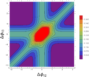
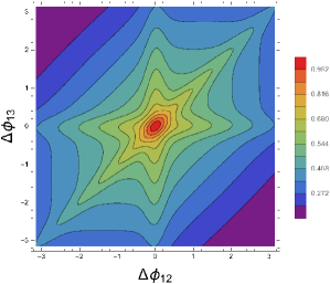
Figure 1: Contour-plots of $c_{3}(\Delta\phi_{12},\Delta\phi_{13})$ with $\Delta y_{12}=\Delta y_{13}=0$ for a two-step cascade (left) as found in [13], and for a three-step cascade obtained in this work (right). The set of parameters used are given in the text.

- for single hidden source:

$$h^{\rm(1)}(\Delta\phi_{12},\Delta\phi_{13})\ \sim\ \frac{1}{\langle N_{{\rm c}}^{{\rm s}}\rangle^{2}}\ \exp{\left[-\frac{(\Delta\phi_{12})^{2}+(\Delta\phi_{13})^{2}-\Delta\phi_{12}\Delta\phi_{13}}{3\delta_{\phi}^{2}}\right]}$$ (11)

$$+\ \frac{1}{\langle N_{{\rm c}}^{{\rm s}}\rangle}\ \exp{\left[-\frac{(\Delta\phi_{12})^{2}+(\Delta\phi_{13})^{2}-\Delta\phi_{12}\Delta\phi_{13}}{2\delta_{{\rm c}\phi}^{2}}\right]}\$$

$$\times\ \left(\exp{\left[-\frac{(\Delta\phi_{12})^{2}}{4\delta_{\phi}^{2}}\right]}+\exp{\left[-\frac{(\Delta\phi_{13})^{2}}{4\delta_{\phi}^{2}}\right]}+\exp{\left[-\frac{(\Delta\phi_{12})^{2}+(\Delta\phi_{13})^{2}-2\Delta\phi_{12}\Delta\phi_{13}}{4\delta_{\phi}^{2}}\right]}\right)$$

$$+\ \exp{\left[-\frac{(\Delta\phi_{12})^{2}+(\Delta\phi_{13})^{2}-\Delta\phi_{12})\Delta\phi_{13})}{3\delta_{{\rm c}\phi}^{2}}\right]}$$

$$+\ \exp{\left[-\frac{(\Delta\phi_{12})^{2}}{2\delta_{{\rm c}\phi}^{2}}\right]}+\exp{\left[-\frac{(\Delta\phi_{12})^{2}}{2\delta_{{\rm c}\phi}^{2}}\right]}+\exp{\left[-\frac{(\Delta\phi_{12})^{2}+(\Delta\phi_{13})^{2}-2\Delta\phi_{12}\Delta\phi_{13}}{2\delta_{{\rm c}\phi}^{2}}\right]}$$

- for two hidden sources:

$$h^{\rm(2)}(\Delta\phi_{12},\Delta\phi_{13})\ \sim\ \left(\frac{1}{\langle N_{{\rm c}}^{{\rm s}}\rangle}\exp{\left[-\frac{(\Delta\phi_{12})^{2}+(\Delta\phi_{13})^{2}-\Delta\phi_{12}\Delta\phi_{13}}{2\delta_{{\rm c}\phi}^{2}+\delta_{{\rm s}\phi}^{2}}\right]}\right.$$

$$\left.+\ \exp{\left[-\frac{(\Delta\phi_{12})^{2}+(\Delta\phi_{13})^{2}-\Delta\phi_{12}\Delta\phi_{13}}{3\delta_{{\rm c}\phi}^{2}+2\delta_{{\rm s}\phi}^{2}}\right]}\right)$$ (12)

$$\times\ \left(\exp{\left[-\frac{(\Delta\phi_{12})^{2}}{4\delta_{\phi}^{2}}\right]}+\exp{\left[-\frac{(\Delta\phi_{13})^{2}}{4\delta_{\phi}^{2}}\right]}+\exp{\left[-\frac{(\Delta\phi_{12})^{2}+(\Delta\phi_{13})^{2}-2\Delta\phi_{12}\Delta\phi_{13}}{4\delta_{\phi}^{2}}\right]}\right)$$

- for three hidden sources:

$$h^{\rm(3)}(\Delta\phi_{12},\Delta\phi_{13})\ \sim\ \exp{\left[-\frac{(\Delta\phi_{12})^{2}+(\Delta\phi_{13})^{2}-\Delta\phi_{12}\Delta\phi_{13}}{3\delta_{{\rm c}\phi}^{2}+\delta_{{\rm s}\phi}^{2}}\right]}$$ (13)

$$+\ \exp{\left[-\frac{(\Delta\phi_{12})^{2}}{2(2\delta_{{\rm c}\phi}^{2}+\delta_{{\rm s}\phi}^{2})}\right]}+\exp{\left[-\frac{(\Delta\phi_{13})^{2}}{2(2\delta_{{\rm c}\phi}^{2}+\delta_{{\rm s}\phi}^{2})}\right]}+\exp{\left[-\frac{(\Delta\phi_{12})^{2}+(\Delta\phi_{13})^{2}-2\Delta\phi_{12}\Delta\phi_{13}}{2(2\delta_{{\rm c}\phi}^{2}+\delta_{{\rm s}\phi}^{2})}\right]}\,.$$

Each term in the above expressions can be put in correspondence with another one from the set of Eqs.(3). In fact, Eqs.(11)-(13) represent a generalization of the equivalent expressions in our previous work [13] once a hidden sector is included. Notice also that the key point for the physical consequences to be explored below is not having three (or more) steps of clustering, instead of two, but the fact that the first cluster provides a long-range correlation length throughout the whole chain of subsequent clusters and final particles.

The behaviour of the three-particle correlation function $c_{3}(\Delta\phi_{12},\Delta\phi_{13})$ as a function of the azimuthal differences $\Delta\phi_{12}$ and $\Delta\phi_{13}$ (for $\Delta y_{12}=\Delta y_{13}=0$), as it could be measured experimentally, is shown in Fig. 1. The left panel shows the contour-plot of the $c_{3}$-function corresponding to a (two-step) standard cascade as obtained earlier in [13]. The right panel shows the new result corresponding to a three-step cascade that we identify with the possible existence of a new stage of matter on top of the conventional parton shower yielding final state particles. We tentatively set $\langle N_{{\rm s}}\rangle=2$, $\langle N_{{\rm c}}^{{\rm s}}\rangle=3$ for the average multiplicities. On the other hand, the pressumably large mass of HS particles implies that their velocities should be considerably smaller than those of clusters and final final state particles. Thereby we choose $\delta_{{\rm s}\phi}\simeq\pi$ as a reference value for the correlation length in the transverse plane between HS particles. Besides, there is an overall normalization of the $c_{3}(\Delta\phi_{12},\Delta\phi_{13})$ function to unity at $\Delta\phi_{12}=\Delta\phi_{13}=0$. It is worthwhile remarking too that the main features of the right-hand plot in Fig. 1 remain almost unchanged under reasonable variations of the above-mentioned parameters.

It is not difficult to understand the underlying reason for such different behaviours. Long-range correlations of final-state particles are inherited from a hidden source convoluting with the shorter correlations from clusters, thereby stretching the “radii” of the “spiderweb-type” structure.

On the other hand, the two-dimensional plot corresponding to (pseudo)rapidity intervals remains practically the same (thus not shown in this paper, see [13]). This can be attributed to the fact that long rapidity correlations are already present in the conventional cascade so that an additional HS source in the partonic shower with $\delta_{{\rm s}y}\simeq\delta_{{\rm c}y}$ does not significantly alter the plot.

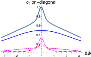
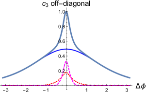
Figure 2: Diagonal (left) and off-digonal (right) projections of the azimuthal contour plot of $c_{3}(\Delta\phi_{12},\Delta\phi_{13})$ from Fig. 1 for a three-step cascade as obtained in this work. The dotted (red), dashed (magenta) and thin solid (blue) curves show the weighted contributions from one, two and three hidden particles, respectively, and the thick (turquoise) curve shows the sum of these contributions.

Figure 2 shows the projection plots of the $c_{3}$ function along the diagonal ($\Delta\phi_{12}=\Delta\phi_{13}$, left panel) and off the diagonal ($\Delta\phi_{12}=-\Delta\phi_{13}$, right panel) under the $\Delta y_{12}=\Delta y_{13}=0$ condition. A different behaviour can again be remarked in both plots, as the on-diagonal correlation length is appreciably longer than the off-diagonal correlation length. The contributions from the different pieces $h^{\rm(1)}$, $h^{\rm(2)}$ and $h^{\rm(3)}$ are also separately shown. Let us observe that the contribution from the $h^{(3)}$ piece is mainly responsible of the “web” structure in the plot.

Summarizing, in this work a potential signature of new physics is shown to be observed in three-particle azimuthal correlations which can be directly tested in experiments at the LHC. Our results can be extended to other than $pp$ collisions. According to our study, the effect of a new stage of matter, as considered here, would manifest as a “web” structure in the three-particle two-dimensional correlation plot in azimuthal space. Such a signature should be considered as complementary to other possible signatures, helpful to discriminate among distinct phenomenologies from Hidden Valley models.

References

[1]
E. A. De Wolf, I. M. Dremin, W. Kittel,
Phys. Rep. 270, 1 (1996)
[arXiv:hep-ph/9508325].
[2]
I. M. Dremin, J. W. Gary,
Phys. Rep. 349, 301 (2001)
[arXiv:hep-ph/0004215].
[3] W. Kittel, E. A. De Wolf, Soft Multihadron Dynamics
(World Scientific, Singapore, 2005).
[4]
M. A. Sanchis-Lozano,
Int. J. Mod. Phys. A 24 (2009) 4529
[arXiv:0812.2397 [hep-ph]].
[5]
K. Dusling, W. Li, B. Schenke,
Int. J. Mod. Phys. E 25, 1630002 (2016)
[arXiv:1509.07939 [nucl-ex]].
[6]
M. J. Strassler and K. M. Zurek,
Phys. Lett. B 651, 374 (2007)
[arXiv:hep-ph/0604261].
[7]
J. Kang and M. A. Luty,
J. High Energy Phys. 0911 (2009) 065
[arXiv:0805.4642 [hep-ph]].
[8]
M. J. Strassler,
arXiv:0806.2385 [hep-ph].
[9]
S. Alekhin et al.,
Rep. Prog. Phys. 79 (2016) 124201
[arXiv:1504.04855 [hep-ph]].
[10]
Y. Nakai, M. Reece and R. Sato,
J. High Energy Phys. 1603 (2016) 143
[arXiv:1511.00691 [hep-ph]].
[11]
S. Knapen, S. Pagan Griso, M. Papucci and D. J. Robinson,
J. High Energy Phys. 1708, 076 (2017)
[arXiv:1612.00850 [hep-ph]].
[12]
T. Cohen, M. Lisanti, H. K. Lou and S. Mishra-Sharma,
J. High Energy Phys. 1711, 196 (2017)
[arXiv:1707.05326 [hep-ph]].
[13]
M.-A. Sanchis-Lozano and E. Sarkisyan-Grinbaum,
Phys. Rev. D 96, 074012 (2017)
[arXiv:1706.05231 [hep-ph]].
[14]
M.-A. Sanchis-Lozano, E. K. Sarkisyan-Grinbaum, S. Moreno-Picot,
Phys. Lett. B 754 (2016) 353
[arXiv:1510.08738 [hep-ph]].
[15]
M.-A. Sanchis-Lozano and E. Sarkisyan-Grinbaum,
Phys. Lett. B 766, 170 (2017)
[arXiv:1610.06408 [hep-ph]].
[16]
C. Bierlich, G. Gustafson and L. Lönnblad,
Phys. Lett. B 779 (2018) 58
[arXiv:1710.09725 [hep-ph]].
[17]
Ş. Özönder,
Phys. Rev. D 91 (2015) 034005
[arXiv:1409.6347 [hep-ph]].
[18]
A. Białas, K. Fiałkowski and K. Zalewski,
Phys. Lett. B 45, 337 (1973).