The Complexity of Drawing a Graph in a Polygonal Region

Abstract

We prove that the following problem is complete for the existential theory of the reals: Given a planar graph and a polygonal region, with some vertices of the graph assigned to points on the boundary of the region, place the remaining vertices to create a planar straight-line drawing of the graph inside the region. A special case is the problem of extending a partial planar graph drawing, which was proved NP-hard by Patrignani. Our result is one of the first showing that a problem of drawing planar graphs with straight-line edges is hard for the existential theory of the reals. The complexity of the problem is open for a simply connected region.

We also show that, even for integer input coordinates, it is possible that drawing a graph in a polygonal region requires some vertices to be placed at irrational coordinates. By contrast, the coordinates are known to be bounded in the special case of a convex region, or for drawing a path in any polygonal region.

1 Introduction

There are many examples of structural results on graphs leading to beautiful and efficient geometric representations. Two highlights are: Tutte’s polynomial-time algorithm [30] to draw any 3-connected planar graph with convex faces inside any fixed convex drawing of its outer face; and Schnyder’s tree realizer result [27] that provides a drawing of any $n$-vertex planar graph on an $n\times n$ grid.

On the other hand, there are geometric representations that are intractable, either in terms of the required coordinates or in terms of computation time. As an example of the former, a representation of a planar graph as touching disks (Koebe’s theorem) is not always possible with rational numbers, nor even with roots of low-degree polynomials [5]. As an example of the latter, Patrignani considered a generalization of Tutte’s theorem and proved that it is NP-hard to decide whether a graph has a straight-line planar drawing when part of the drawing is fixed [24]. He was unable to show that the problem lies in NP because of coordinate issues.

This, and many other geometric problems, most naturally lie not in NP, but in a larger class, $\exists\mathbb{R}$, defined by formulas in existentially quantified real (rather than Boolean) variables. Showing that a geometric representation problem is complete for $\exists\mathbb{R}$ is a stronger intractability result, often implying lower bounds on coordinate sizes. For example, McDiarmid and Müller [19] showed that deciding if a graph can be represented as intersecting disks is $\exists\mathbb{R}$-complete. The relaxation from touching disks (Koebe’s theorem) to intersecting disks implies that disk centers and radii can be restricted to integers, but McDiarmid and Müller show that an exponential number of bits may be required.

In this paper we prove that an extension of Tutte’s problem is $\exists\mathbb{R}$-complete. We call it the “Graph in Polygon” problem. See Figure 1. The input is a graph $G$ and a closed polygonal region $R$ (not necessarily simply connected), with some vertices of $G$ assigned fixed positions on the boundary of $R$. The question is whether $G$ has a straight-line planar drawing inside $R$ respecting the fixed vertices. We regard the region $R$ as a closed region which means that boundary points of $R$ may be used in the drawing. A straight-line planar drawing (see Figure 2(a,b)) means that vertices are represented as distinct points, and every edge is represented as a straight-line segment joining its endpoints, and no two of the closed line segments intersect except at a common vertex. (In particular, no vertex point may lie inside an edge segment, and no two segments may cross.)

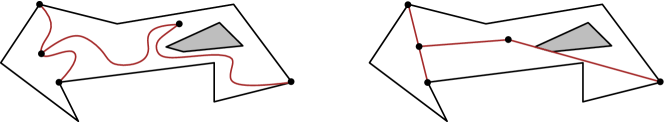
Figure 1: The Graph in Polygon problem. Left: a polygonal region with one hole and a graph to be embedded inside the region. The three vertices on the boundary are fixed; the others are free. Right: a straight-line embedding of the graph in the region. Note that we allow an edge of the drawing (in red) to include points of the region boundary.

Furthermore, we give a simple instance of Graph in Polygon with integer coordinates where a vertex of $G$ may need irrational coordinates in any solution, thus defeating the naive approach to placing the problem in NP.

The Graph in Polygon problem is a very natural one that arises in practical applications such as dynamic and incremental graph drawing. Questions of the coordinates (or grid size) required for straight-line planar drawings of graphs are fundamental and well-studied [32]. It is surprising that a problem as simple and natural as Graph in Polygon is so hard and requires irrational coordinates.

We state our results below, but first we give some background on existential theory of the reals and on relevant graph drawing results. In particular, we explain that our problem is a generalization of the problem of extending a partial drawing of a planar graph to a straight-line drawing of the whole graph, called Partial Drawing Extensibility. See Figure 2(c,d).

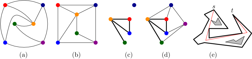
Figure 2: (a) A planar graph $G$. (b) A straight-line drawing of $G$. (c) A partial drawing $\Gamma$ of $G$. (d) Extension of $\Gamma$ to a straight-line drawing of $G$. (e) A minimum-link $s$-$t$ path in a polygonal region.

Existential Theory of the Reals. In the study of geometric problems, the complexity class $\exists\mathbb{R}$ plays a crucial role, connecting purely geometric problems and real algebra. Whereas NP is defined in terms of Boolean formulas in existentially quantified Boolean variables, $\exists\mathbb{R}$ deals with first-order formulas in existentially quantified real variables.

Consider a first-order formula over the reals that contains only existential quantifiers, $\exists x_{1},x_{2},\ldots,x_{n}:$ $\Phi(x_{1},x_{2},\ldots,x_{n})$, where $x_{1},x_{2},\ldots,x_{n}$ are real-valued variables and $\Phi$ is a quantifier-free formula involving equalities and inequalities of real polynomials. The Existential Theory of the Reals (ETR) problem takes such a formula as an input and asks whether it is satisfiable. The complexity class $\exists\mathbb{R}$ consists of all problems that reduce in polynomial time to ETR. Many problems in combinatorial geometry and geometric graph representation naturally lie in this class, and furthermore, many have been shown to be $\exists\mathbb{R}$-complete, e.g., stretchability of a pseudoline arrangement [18, 22, 26], recognition of segment intersection graphs [17] and disk intersection graphs [19], computing the rectilinear crossing number of a graph [6], etc. For surveys on $\exists\mathbb{R}$, see [25, 8, 18]. A recent proof that the Art Gallery Problem is $\exists\mathbb{R}$-complete [2] provides the framework we follow in our proof.

Planar Graph Drawing. The field of Graph Drawing investigates many ways of representing graphs geometrically [23], but we focus on the most basic representation of planar graphs, with points for vertices and straight-line segments for edges, such that segments intersect only at a common endpoint. By Fáry’s theorem [12], every planar graph admits such a straight-line planar drawing.

In Tutte’s famous paper, “How to Draw a Graph,” he gave a polynomial time algorithm to find a straight-line planar drawing of a graph by first augmenting to a 3-connected graph. Given a combinatorial planar embedding (a specification of the faces) of a 3-connected graph and given a convex polygon drawing of the outer face of the graph, his algorithm produces a planar straight-line drawing respecting both by reducing the problem to solving a linear system involving barycentric coordinates for each internal vertex. Tutte proved that the linear system has a unique solution and that the solution yields a drawing with convex faces. The linear system can be solved in polynomial time. For a discussion of coordinate bit complexity see Section 4.

There is a rich literature on implications and variations of Tutte’s result. We concentrate on the aspects of drawing a planar graph in a constrained region, or when part of the drawing is fixed. (We leave aside, for example, the issue of drawing graphs with convex faces, which also has an extensive literature.)

Our focus will be on straight-line planar graph drawings, but it is worth mentioning that without the restriction to straight-line drawings, the problem of finding a planar drawing of a graph (with polygonal curves for edges) in a constrained region is equivalent to the problem of extending a partial planar drawing (with polygonal curves for edges), and there is a polynomial time algorithm for the decision version of the problem [3]. Furthermore, there is an algorithm to construct such a drawing in which each edge is represented by a polygonal curve with linearly many segments [10].

For the rest of this paper we assume straight-line planar drawings, which makes the problems harder. The problem of drawing a graph in a constrained region is formalized as Graph in Polygon, defined above, and more precisely in Subsection 1.1. The problem of finding a planar straight-line drawing of a graph after part of the drawing has been fixed is called Partial Drawing Extensibility in the literature—its complexity was formulated as an open question in [7].

The relationship between the two problems is that Graph in Polygon generalizes Partial Drawing Extensibility, as we now argue. Given an instance of partial drawing extensibility, for graph $G$ with fixed subgraph $H$, we construct an instance of Graph in Polygon by making a point hole for each vertex of $H$ and assigning the vertex to the point. Then an edge of $H$ can only be drawn as a line segment joining its endpoints, so we have effectively fixed $H$. To complete the bounded region $R$, we enclose the point holes in a large box. Clearly, we now have an instance of Graph in Polygon, and that instance has a solution if and only if $G$ has a planar straight-line drawing that extends the drawing of $H$. There is no easy reduction in the other direction because Graph in Polygon involves a closed polygonal region, so an edge may be drawn as a segment that touches, or lies on, the boundary of the region, and it is not clear how to model this as Partial Drawing Extensibility. However, the version of Graph in Polygon for an open region is equivalent to Partial Drawing Extensibility.

We now summarize results on Partial Drawing Extensibility, beginning with positive results. Besides Tutte’s result that a convex drawing of the outer face can always be extended, there is a similar result for a star-shaped drawing of the outer face [14]. There is also a polynomial-time algorithm to decide the case when a convex drawing of a subgraph is fixed [20]. Urhausen [31] examined the case when a star-shaped drawing of one cycle in the graph is given, and proved that there always exists an extension with at most one bend per edge. Gortler et al. [13] gave an algorithm, extending Tutte’s algorithm, that succeeds in some (not well-characterized) cases for a simple non-convex drawing of the outer face. The Partial Drawing Extensibility problem was shown to be NP-hard by Patrignani [24]. This implies that Graph in Polygon is NP-hard. However, there are two natural questions about partial drawing extensibility that remain open: (a) does the problem belong to the class NP (discussed in detail by Patrignani [24]), and (b) does the problem remain NP-hard when a combinatorial embedding of the graph is given and must be respected in the drawing. Our results shed light on these questions for the more general Graph in Polygon problem: the problem cannot be shown to lie in NP by means of giving the vertex coordinates, and the problem is still $\exists\mathbb{R}$-hard when a combinatorial embedding of the graph is given.

Besides Tutte’s result, there is another special case of Graph in Polygon that is well-solved, namely when the graph is just a path with its two endpoints $s$ and $t$ fixed on the boundary of the region. See Figure 2(e). This problem is equivalent to the Minimum Link Path problem—to find a path from $s$ to $t$ inside the region with a minimum number of segments. This is because a path of $k$ edges can be drawn inside the region if and only if the minimum link distance between $s$ and $t$ is less than or equal to $k$. Minimum link paths in a polygonal region can be found in polynomial time [21], and in linear time for a simple polygon [28]. The complexity of the coordinates is well-understood (see Section 4).

1.1 Our Contributions

Our problem is defined as follows.

Graph in Polygon

Input: A planar graph $G$ and a polygonal region $R$ with some vertices of $G$ assigned to fixed positions on the boundary of $R$.

Question: Does $G$ admit a planar straight-line drawing inside $R$ respecting the fixed vertices?

The graph may be given abstractly, or via a combinatorial embedding which specifies the cyclic order of edges around each vertex, thus determining the faces of the embedding. When a combinatorial embedding is specified then the final drawing must respect that embedding.

Note that we regard $R$ as a closed region. Thus, points on the boundary of $R$ may be used in the drawing of $G$. In particular, an edge of $G$ may be drawn as a segment that touches, or lies on, the boundary of $R$. See Figure 1. Note that we still require the drawing of $G$ to be “simple” in the conventional sense that no two edge segments may intersect except at a common endpoint.

Our first result is that solutions to Graph in Polygon may involve irrational points. This will in fact follow from the proof of our main hardness result, but it is worth seeing a simple example.

Theorem 1.1 ()

There is an instance of Graph in Polygon with all coordinates given by integers, in which some vertices need irrational coordinates.

Note that the theorem does not rule out membership of the problem in NP, since it may be possible to demonstrate that a graph can be drawn in a region without giving explicit vertex coordinates. We prove Theorem 1.1 by adapting an example from Abrahamsen, Adamaszek and Miltzow [1] that proves a similar irrationality result for the Art Gallery Problem. Further discussion of bit complexity for special cases of the problem can be found in Section 4.

Our main result is the following, which holds whether the graph is given abstractly or via a combinatorial embedding.

Theorem 1.2 ()

Graph in Polygon is $\exists\mathbb{R}$-complete.

We prove Theorem 1.2 using a reduction from a problem called ETR-INV which was introduced and proved $\exists\mathbb{R}$-complete by Abrahamsen, Adamaszek and Miltzow [2].

Definition 1 (ETR-INV)

In the problem ETR-INV, we are given a set of real variables $\{x_{1},\ldots,x_{n}\}$, and a set of equations of the form $x=1,\quad x+y=z,\quad x\cdot y=1,$ for $x,y,z\in\{x_{1},\ldots,x_{n}\}$. The goal is to decide whether the system of equations has a solution when each variable is restricted to the range $[1/2,2]$.

Reducing from ETR-INV, rather than from ETR, has several crucial advantages. First, we can assume that all variables are in the range $[1/2,2]$. Second, we do not have to implement a gadget that simulates multiplication, but only inversion, i.e., $x\cdot y=1$. For our purpose of reducing to Graph in Polygon, we will find it useful to further modify ETR-INV to avoid equality and to ensure planarity of the variable-constraint incidence graph, as follows:

Definition 2 ($\textrm{Planar-ETR-INV}^{*}$)

In the problem $\textrm{Planar-ETR-INV}^{*}$, we are given a set of real variables $\{x_{1},\ldots,x_{n}\}$, and a set of equations and inequalities of the form $x=1\text{, }x+y\leq z\text{, }x+y\geq z\text{, }x\cdot y\leq 1\text{, }x\cdot y\geq 1\text{, }\text{ for }x,y,z\in\{x_{1},\ldots,x_{n}\}.$ Furthermore, we require planarity of the variable-constraint incidence graph, which is the bipartite graph that has a vertex for every variable and every constraint and an edge when a variable appears in a constraint. The goal is to decide whether the system of equations has a solution when each variable is restricted to lie in $[1/2,4]$.

As a technical contribution, we prove the following.

Theorem 1.3 ()

$\textrm{Planar-ETR-INV}^{*}$ is $\exists\mathbb{R}$-complete.

The proof, which is in Appendix 0.A, builds on the work of Dobbins, Kleist, Miltzow and Rzażewski [11] who showed that ETR-INV is $\exists\mathbb{R}$-complete even when the variable-constraint incidence graph is planar. We cannot use their result directly, but follow similar steps in our proof.

2 Irrational Coordinates

See 1.1

In fact, the result follows from our proof of Theorem 1.2, but it is interesting to have a simple explicit example, which is given in Figure 4. This example is adapted from a result of Abrahamsen et al. [1]. Details can be found in Appendix 0.B, but we outline the idea here. Abrahamsen et al. studied the Art Gallery Problem, where given a polygon $P$ and a number $k$, and we want to find a set of at most $k$ guards (points) that together see the entire polygon. We say a guard $g$ sees a point $p$ if the entire line-segment $gp$ is contained inside the polygon $P$. Abrahamsen et al. gave a simple polygon with integer coordinates such that there exists only one way to guard it optimally, with three guards. Those guards have irrational coordinates. See Figure 3 for a sketch of their polygon. A key ingredient of their construction is to create notches in the polygon boundary that force there to be a guard on each of the three so-called guard segments. The coordinates of the polygon then force the guards to be at irrational points.

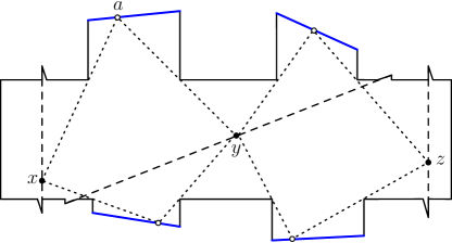
Figure 3: A sketch of the polygon from Abrahamsen et al. The three guards (black dots) must lie on the guard segments (dashed lines).

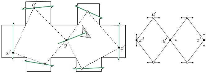
Figure 4: Left: An instance of Graph in Polygon based on Figure 3 that requires vertices at irrational coordinates. Right: The graph, with small dots indicating the fixed vertices.

We adapt their example by using variable segments (shown in green) instead of guard segments, and vertices instead of guards. By placing notches in the polygon boundary with fixed vertices of the graph in the notches, we can force there to be a vertex on each variable segment. We create two cycles that replicate the guarding constraints, and use a hole in order to keep our graph drawing planar. From their proof we show that $x^{\prime}$, $y^{\prime}$ and $z^{\prime}$ must be at irrational coordinates.

3 $\exists\mathbb{R}$-completeness

See 1.2

Proof

First note that Graph in Polygon lies in $\exists\mathbb{R}$ since we can express it as an ETR formula. To prove that the problem is $\exists\mathbb{R}$-hard we give a reduction from $\textrm{Planar-ETR-INV}^{*}$. Let $I$ be an instance of $\textrm{Planar-ETR-INV}^{*}$. We will build an instance $J$ of Graph in Polygon such that $J$ admits an affirmative answer if and only if $I$ is satisfiable. The idea is to construct gadgets to represent variables, and gadgets to enforce the addition and inversion inequalities, $x+y\leq z,x+y\geq z,x\cdot y\leq 1,x\cdot y\geq 1$. We also need gadgets to copy and replicate variables—“wires” and “splitters” as conventionally used in reductions. Thereafter, we have to describe how to combine those gadgets to obtain an instance $J$ of $\textrm{Planar-ETR-INV}^{*}$.

Encoding Variables. We will encode the value of a variable in $[1/2,4]$ as the position of a vertex that is constrained to lie on a line segment of length $3.5$, which we call a variable-segment. One end of a variable-segment encodes the value $\frac{1}{2}$, the other end encodes the value $4$, and linear interpolation fills in the values between. Figure 5 shows one side of the construction that forces a vertex to lie on a variable-segment. The other side is similar.

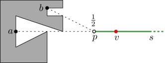
Figure 5: Variable $v$ is represented as a point on variable-segment $s$ (shown in green). The construction of one end of $s$ is illustrated. In the graph, vertex $v$ is adjacent to fixed vertices $a$ and $b$ on the boundary of a hole of the region (shaded). Adjacency with $a$ forces $v$ to lie on the line of $s$. Adjacency with $b$ forces $v$ to lie at, or to the right of, point $p$ which is associated with the value $1/2$. Note that $p$ is not a vertex.

By slight abuse of notation, we will identify a variable and the vertex representing it, if there is no ambiguity. For the description of the remaining gadgets, our figures will show variable-segments (in green) without showing the polygonal holes that determine them.

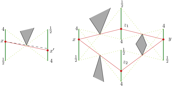
Figure 6: Copying. Left: a gadget to enforce $x{\leq}x^{\prime}$. Right: The full gadget enforcing $x{=}y$.

Copy gadget. Given a variable-segment for a variable $x$, we will need to transmit its value along a “wire” to other locations in the plane. We do this using a copy gadget in which we construct a variable-segment for a new variable $y$ and enforce $x=y$. We show how to construct a gadget that ensures $x\leq x^{\prime}$ for a new variable $x^{\prime}$, and then combine four such gadgets, enforcing $x\leq z_{1},z_{1}\leq y,x\geq z_{2},z_{2}\geq y$. This implies $x=y$.

The gadget enforcing $x\leq x^{\prime}$ is shown at the left of Figure 6. It consists of two parallel variable-segments. In general, these two segments need not be horizontally aligned. In the graph we connect the corresponding vertices by an edge. The left and the right variables are encoded in opposite ways, i.e., $x$ increases as the vertex moves up and $x^{\prime}$ increases as the corresponding vertex goes down. We place a hole of the polygonal region (shaded in the figure) with a vertex at the intersection point of the lines joining the top of one variable-segment to the bottom of the other. The hole must be large enough that the edge from $x$ to $x^{\prime}$ can only be drawn to one side of the hole. An argument about similar triangles, or the “intercept theorem”, also known as Thales’ theorem, implies $x\leq x^{\prime}$.

We combine four of these gadgets to construct our copy gadget, as illustrated on the right of Figure 6.

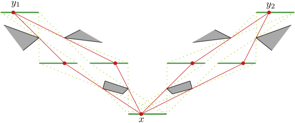
Figure 7: Splitting. The variables $y_{1},y_{2}$ have both the same value as $x$.

Splitter gadget. Since a single variable may appear in several constraints, we may need to split a wire into two wires, each holding the correct value of the same variable. Figure 7 shows a gadget to split the variable $x$ to variables $y_{1}$ and $y_{2}$. The gadget consists of two copy gadgets sharing the variable-segment for $x$. We can construct the two copy gadgets to avoid any intersections between them.

Turn gadget. We need to encode a variable both as a vertical and as a horizontal variable-segment. To transform one into the other we use a turn gadget.

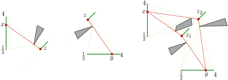
Figure 8: Turning. Left: Gadget to encode $x\leq f(z)$. Middle: Symmetric gadget to encode $y\geq f(z)$. Right: Four gadgets of the previous type combined to enforce $x=y$, for $x$ and $y$ on a vertical and horizontal variable-segment, respectively.

The key idea is to construct two diagonal variable-segments for variables $z_{1}$ and $z_{2}$, and then transfer the value of the vertical variable-segment to the horizontal variable-segment using $z_{1},z_{2}$. This is in fact very similar to the copy gadget, except that the intermediate variable-segments are placed on a line of slope 1. We do not know if it is possible to enforce the constraint $x\leq z$ directly. However, it is sufficient to enforce $x\leq f(z)$ for some function $f$. See the left side of Figure 8. Interestingly, we don’t even know the function $f$. However, we do know that $f$ is monotone and we can construct another gadget enforcing $y\geq f(z)$, for the same function $f$, by making another copy of the first gadget reflected through the line of the variable-segment for $z$.

Combining four such gadgets, as on the right of Figure 8, yields the following inequalities: $x\leq f_{1}(z_{1}),f_{1}(z_{1})\leq y,y\leq f_{2}(z_{2}),f_{2}(z_{2})\leq x$. This implies $x=y$.

Addition gadget.

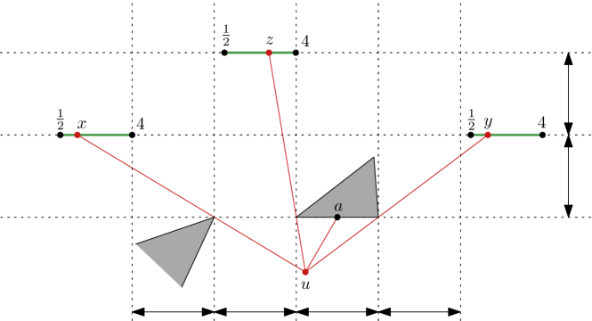
Figure 9: Addition. The three vertices $x,y,z$ can only be connected to $u$ if $x{+}y{\geq}z$ holds.

The gadget to enforce $x+y\geq z$ is depicted in Figure 9. Important for correctness is that the gaps between the dotted auxiliary lines have equal lengths. This is essentially the same gadget that was used by Abrahamsen et al. [2, Lemma 31]. We offer an alternative correctness proof, which is in Appendix 0.C.

Lemma 1 ([2])

The gadget in Figure 9 enforces $x+y\geq z$.

The gadget that enforces $x+y\leq z$ is just a mirror copy of the previous gadget.

Inversion gadget. The inversion gadgets to enforce $x\cdot y\leq 1$ and $x\cdot y\geq 1$ are depicted in Figure 10. We use a horizontal variable-segment for $x$ and a vertical variable-segment for $y$ and align them as shown in the figure, $1.5$ units apart both horizontally and vertically. We make a triangular hole with its apex at point $q$ as shown in the figure. The graph has an edge between $x$ and $y$.

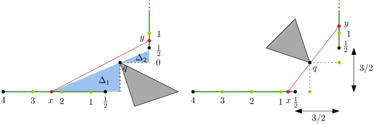
Figure 10: Inversion. Left: Gadget enforcing $x\cdot y\geq 1$. Right: Gadget enforcing $x\cdot y\leq 1$.

For correctness, observe that if $x$ and $y$ are positioned so that the line segment joining them goes through point $q$, then, because triangles $\Delta_{1}$ and $\Delta_{2}$ (as shown in the figure) are similar, we have $\frac{x}{1}=\frac{1}{y}$, i.e. $x\cdot y=1$. If the line segment goes above point $q$ (as in the left hand side of Figure 10) then $x\cdot y\geq 1$, and if the line segment goes below then $x\cdot y\leq 1$.

Putting it all together. It remains to show how to obtain an instance of Graph in Polygon in polynomial time from an instance of $\textrm{Planar-ETR-INV}^{*}$.

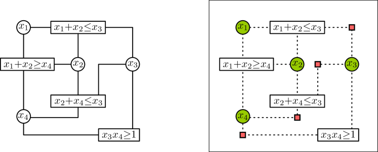
Figure 13: The overall reduction from $\textrm{Planar-ETR-INV}^{*}$ to Graph in Polygon. Left: A rectilinear drawing $D$ of the variable-constraint graph of $I$. In this example every variable vertex has degree at most $3$. Right: A schematic representation of the resulting instance. The variable-segments are placed inside the variable vertices (green). Every edge is replaced by a sequence of copy gadgets (dotted lines) and turn gadgets (red squares). The constraint vertices are replaced by the corresponding constraint gadgets. Note that it might be necessary to have one or several turn and copy gadgets as part of the addition and inversion gadgets.

Let $I$ be an instance of $\textrm{Planar-ETR-INV}^{*}$. As a first step we modify the planar variable-constraint incidence graph so that a variable vertex of degree $d$ is replaced by “splitter” vertices of degree at most 3 to create $d$ copies. Then we compute a plane rectilinear drawing $D$ of the resulting planar graph, which can be done in polynomial time using rectilinear planar drawing algorithms [23]. The edges of $D$ act as wires and we replace each horizontal and vertical segment by a copy gadget, and replace every $90$ degree corner, by a turn gadget. Every splitter vertex and constraint vertex will be replaced by the corresponding gadget, possibly using turn gadgets. We add a big square to the outside, to ensure that everything is inside one polygon. See Figure 13 in Appendix 0.C.

It is easy to see that this can be done in polynomial time, as every gadget has a constant size description and can be described with rational numbers, although, we did not do it explicitly. In order to see that we can also use integers, note that we can scale everything with the least common multiple of all the denominators of all numbers appearing. This can also be done in polynomial time. ∎

4 Vertex Coordinates

Since we have shown that Graph in Polygon may require irrational coordinates for vertices in general, it is interesting to examine bounds on coordinates for special cases. In this section we discuss the bit complexity of vertex coordinates needed for two well-solved special cases of Graph in Polygon.

Tutte’s algorithm [29] finds a straight-line planar drawing of a graph inside a fixed convex drawing of its outer face. Suppose the graph has $n$ vertices and each coordinate of the convex polygon uses $t$ bits. Tutte’s algorithm runs in polynomial time, but the number of bits used to express the vertex coordinates is a polynomial function of $t$ and $n$. The dependence on $n$ means that the drawing uses “exponential area.” Chambers et al. [9] gave a different algorithm that uses polynomial area—the number of bits for the vertex coordinates is bounded by a polynomial in $t$ and $\log n$.

The other well-solved case of Graph in Polygon is the minimum link path problem. Here we have a general polygonal region with holes, $R$, but the graph is restricted to a path with endpoints $s$ and $t$ fixed on the boundary of $R$. Based on a lower bound result of Kahan and Snoeyink [15], Kostitsyna et al. [16] proved a tight bound of $\Theta(n\log n)$ bits for the coordinates of the bends on a minimum link path. Note that the dependence on $n$ means that this bound is exponentially larger than the bound for drawing a graph inside a convex polygon. Problem 3 below asks about the complexity of drawing a tree in a polygonal region.

5 Conclusion and Open Questions

Our result that Graph in Polygon is $\exists\mathbb{R}$-complete is one of the first $\exists\mathbb{R}$-hardness results about drawing planar graphs with straight-line edges—along with a recent result about drawings with prescribed face areas [11]. We conclude with some open questions:

1. Our proofs of Theorems 1.1 and 1.2 used the fact that the polygonal region may have holes and may have collinear vertices. Is Graph in Polygon polynomial-time solvable for a simple polygon (a polygonal region without holes) whose vertices lie in general position (without collinearities)?

2. Our proofs also used the assumption that the polygonal region is closed. For an open region, the problem Graph in Polygon is equivalent to the problem Partial Drawing Extensibility. Is this problem $\exists\mathbb{R}$-hard? There are two versions, depending on whether the graph is given abstractly or via a combinatorial embedding. In the first case the problem is known to be NP-hard [24], but in the second case even that is not known.

3. What is the complexity of Graph in Polygon when the graph is a tree? Can vertex coordinates still be bounded as for the minimum link path problem? When the tree is a caterpillar, the problem might be related to the minimum link watchman tour problem, which is known to be NP-hard [4].

5.0.1 Acknowledgment.

We would like to thank Günter Rote, who discussed with the second author the turn gadget in the context of the Art Gallery Problem.

Appendix 0.A $\textrm{Planar-ETR-INV}^{*}$ is $\exists\mathbb{R}$-complete

The purpose of this section is to prove Theorem 1.3. See 1.3

Our proof builds on the work of Dobbins, Kleist, Miltzow and Rzażewski [11]. They showed that ETR-INV is $\exists\mathbb{R}$-complete even when the variable-constraint incidence graph is planar. We cannot simply start from their result, because we still need to eliminate equalities, and the obvious idea of replacing $x+y=z$ (for example) by two constraints of the form $x+y\leq z$ and $x+y\geq z$ will destroy planarity of the variable-constraint incidence graph.

Proof

First note that $\textrm{Planar-ETR-INV}^{*}$ is in $\exists\mathbb{R}$ since it is expressible as ETR.

To prove $\exists\mathbb{R}$-hardness we reduce from ETR-INV. For this purpose let $I$ be an instance of ETR-INV. As first step we replace every equality constraint by the two corresponding inequality constraints. For the next step, let $G_{I}$ be the variable-constraint graph of $I$. Let $D$ be a drawing of $G_{I}$ in the plane with edges drawn as straight line segments and vertices represented by points. We assume that no three segments cross in a common point. This drawing may have crossing edges. We will add constraints and variables to $I$ to obtain a new instance $J$, which is equivalent to $I$ and such that the corresponding graph $G_{J}$ is planar. To compute $J$, we replace each crossing in $D$ by a ‘crossing gadget’. Since $D$ has at most a quadratic number of crossings, this construction takes polynomial time.

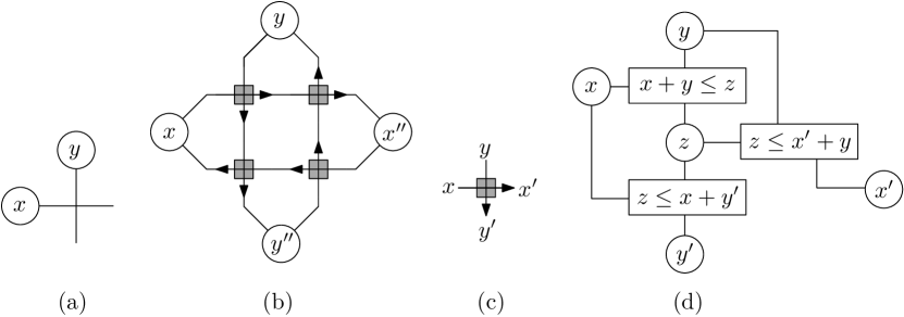
Figure 11: A crossing gadget: (a) a crossing; (b) a crossing gadget composed of 4 half-crossing gadgets that enforces $x=x^{\prime\prime}$ and $y=y^{\prime\prime}$; (c) schematic of a half-crossing gadget; (d) detail of a half-crossing gadget that ensures $x\leq x^{\prime}$ and $y\leq y^{\prime}$.

We first introduce a half-crossing gadget that almost does the job, by using an idea of Dobbins et al. [11]. Figure 11(d) illustrates this gadget. Note that the inequalities $x+y\leq z$ and $z\leq x^{\prime}+y$ ensure that $x\leq x^{\prime}$. Similarly, we can observe that $y\leq y^{\prime}$.

To enforce $x=x^{\prime\prime}$ and $y=y^{\prime\prime}$ we use four copies of the half-crossing gadget to build a crossing gadget. See Figure 11(b). The top two half-crossing gadgets (i.e., the pair of gadgets lying on the $x$-monotone path from $x$ to $x^{\prime\prime}$) ensure $x\leq x^{\prime\prime}$. The bottom two half-crossing gadgets ensure $x\geq x^{\prime\prime}$. Together they ensure $x=x^{\prime\prime}$. The same works with $y$ and $y^{\prime\prime}$.

Since the variables of ETR-INV are restricted to the range $[1/2,2]$, the variable $z$ will lie in the interval $[1,4]$. This is why our definition of $\textrm{Planar-ETR-INV}^{*}$ involved a larger range for variables. Accordingly, our final step is to loosen the range restriction of all variables to $[1/2,4]$. For any new variable $z$ introduced in a half-crossing gadget, the larger range does no harm. For any original variable $x$, we will enforce the added restriction that $x\leq 2$ by adding further constraints. In particular, add two new variables $a_{x}$ and $b_{x}$ and add the constraints $a_{x}=1$, $b_{x}=1$, $a_{x}+b_{x}\geq x$. Note that the variable-constraint incidence graph remains planar, since the new constraints and variables only connect to $x$ in the graph.

The final constructed instance $J$ is equivalent to the original, has a planar variable-constraint incidence graph, and restricts all variables to the required range. ∎

Appendix 0.B Additional Details of Irrational Coordinates

This section heavily relies on a paper by Abrahamsen et al. [1]. We repeat the key ideas of their paper and show how to adapt it for our purpose. In their paper, they studied the Art Gallery Problem. In the Art Gallery Problem, we are given a polygon $P$ and a number $k$, and we want to find a set of at most $k$ guards (points) that together see the entire polygon. We say a guard $g$ sees a point $p$ if the entire line-segment $gp$ is contained inside the polygon $P$. Abrahamsen et al. gave a simple polygon with integer coordinates such that there exists only one way to guard it optimally, with three guards. Those guards have irrational coordinates. See Figure 3, for a sketch of their polygon.

The key ingredients of their proof are as follows. First observe that the notches in the polygon boundary force there to be a guard on each of the three so-called guard segments, indicated by the dashed lines. Then the left guard and the middle guard together must see the top left pocket edge and bottom left pocket edge (shown in blue). Similarly the middle guard and the right guard together must see the top right pocket edge and bottom right pocket edge. Abrahamsen et al. specify precise coordinates for the polygon that force unique positions for the guards, and such that those positions have irrational coordinates. As shown in Figure 3, the unique guard positions result in a single point on each pocket edge that is seen by two guards. For example, point $a$ is the only point on the top left pocket edge that is seen by $x$ and $y$. In particular, the line segments $xa$ and $ya$ pass through reflex corners of the polygon.

We adopt this example as follows, see Figure 4. Instead of guard segments we use variable segments (shown in green), and instead of guards we use vertices. We describe variable segments in detail in Section 3, see also Figure 5. By placing notches in the polygon boundary with fixed vertices of the graph in the notches, we can force there to be a vertex on each variable segment. The pocket edges of the previous example become variable segments. The middle variable segment, the one that contains vertex $y^{\prime}$ in the figure, is determined by a hole in the region. We need to use a hole in order to keep our graph drawing planar. Note that, besides the fixed vertices lying on the boundary of the region, our graph now has 7 vertices, which are forced to lie on 7 distinct variable segments. To complete the construction of our graph, we add edges between the 7 vertices to create two cycles: one containing the leftmost four vertices and the other containing the rightmost four vertices, as illustrated by the dotted lines in Figure 4.

Now the constraints on the three vertices $x^{\prime}$, $y^{\prime}$ and $z^{\prime}$, shown with black dots in Figure 4, are exactly the same as for the guards $x$, $y$, and $z$ in Figure 3. All that changes is how the constraints are described. Let us give an explicit example. The guards $x$ and $y$ together need to see the top left pocket edge. In our new polygon, the vertices $x^{\prime}$ and $y^{\prime}$ must both be adjacent to the same vertex $a^{\prime}$, as indicated in Figure 4. This imposes the same constraints on the vertices $x^{\prime},y^{\prime}$ as was imposed on the guards $x,y$. This translation of conditions happens in the same way for all the other pockets.

As there exists only one position to guard Abrahamsen et al.’s polygon with three guards, there exists also only one way to place the vertices in the polygon of Figure 4, and those positions are irrational.

Appendix 0.C Additional Details for $\exists\mathbb{R}$-completeness

Proof (Proof of Lemma 1)

This proof is inspired by the following thought experiment. Assuming that we choose $z$ always to be the maximum possible value. Furthermore we assume that while we fix the position of $y$, we move $x$ some distance $d$ to the left. What we would expect is that $z$ moves by the same distance to the left. Actually, showing the last statement also proves the lemma, due to symmetry of $x$ and $y$. We denote by $\ell$ the line that contains the variable segments of $x$ and $y$. We denote by $t$ half the distance that $z$ moves. Note that $t$ has a geometric interpretation as indicated in Figure 12. We need to show $d=2t$. The lengths $A,A^{\prime},B,B^{\prime}$ are defined, by Figure 12. Note that $B^{\prime}=2B$, because $\|a-b\|=\|b-c\|$. Similarly, follows $A^{\prime}=2A$. The lemma follows from

$$d=B^{\prime}-A^{\prime}=2(B-A)=2t.$$

∎

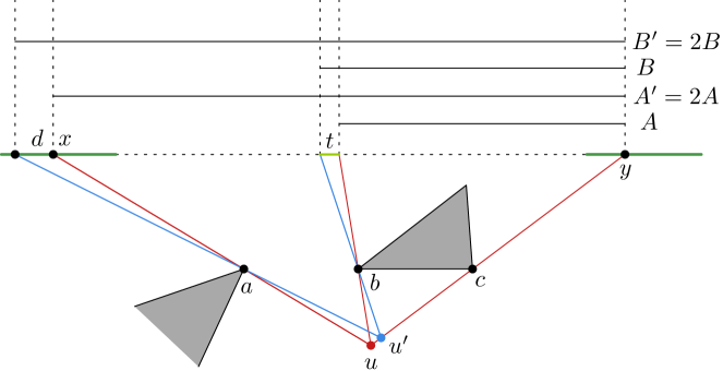
Figure 12: An illustration of the correctness of the addition gadget.

References

- [1] Abrahamsen, M., Adamaszek, A., Miltzow, T.: Irrational guards are sometimes needed. In: Proceedings of the 33rd International Symposium on Computational Geometry (SoCG). pp. 3:1–3:15. LIPIcs (2017)
- [2] Abrahamsen, M., Adamaszek, A., Miltzow, T.: The art gallery problem is -complete. In: Proceedings of the 50th Annual ACM SIGACT Symposium on Theory of Computing, STOC 2018, Los Angeles, CA, USA, June 25-29, 2018. pp. 65–73 (2018), http://doi.acm.org/10.1145/3188745.3188868
- [3] Angelini, P., Di Battista, G., Frati, F., Jelínek, V., Kratochvíl, J., Patrignani, M., Rutter, I.: Testing planarity of partially embedded graphs. ACM Transactions on Algorithms 11(4), 32:1–32:42 (2015)
- [4] Arkin, E.M., Mitchell, J.S.B., Piatko, C.D.: Minimum-link watchman tours. Information Processing Letters 86(4), 203–207 (2003)
- [5] Bannister, M.J., Devanny, W.E., Eppstein, D., Goodrich, M.T.: The Galois complexity of graph drawing: Why numerical solutions are ubiquitous for force-directed, spectral, and circle packing drawings. Journal of Graph Algorithms and Applications 19(2), 619–656 (2015)
- [6] Bienstock, D.: Some provably hard crossing number problems. Discrete & Computational Geometry 6, 443–459 (1991)
- [7] Brandenburg, F., Eppstein, D., Goodrich, M.T., Kobourov, S.G., Liotta, G., Mutzel, P.: Selected open problems in graph drawing. In: Liotta, G. (ed.) Proceedings of the 11th International Symposium on Graph Drawing (GD). LNCS, vol. 2912, pp. 515–539. Springer (2004)
- [8] Cardinal, J.: Computational geometry column 62. ACM SIGACT News 46(4), 69–78 (2015)
- [9] Chambers, E.W., Eppstein, D., Goodrich, M.T., Löffler, M.: Drawing graphs in the plane with a prescribed outer face and polynomial area. Journal of Graph Algorithms and Applications 16(2), 243–259 (2012)
- [10] Chan, T.M., Frati, F., Gutwenger, C., Lubiw, A., Mutzel, P., Schaefer, M.: Drawing partially embedded and simultaneously planar graphs. Journal of Graph Algorithms and Applications 19(2), 681–706 (2015)
- [11] Dobbins, M.G., Kleist, L., Miltzow, T., Rz\polhkażewski, P.: R-completeness and area-universality. In: Brandstädt, A., Köhler, E., Meer, K. (eds.) Proceedings of the 44th International Workshop on Graph-Theoretic Concepts in Computer Science (WG). LNCS, vol. 11159 (2018), http://arxiv.org/abs/1712.05142
- [12] Fáry, I.: On straight line representations of planar graphs. Acta Sci. Math. Szeged 11, 229–233 (1948)
- [13] Gortler, S.J., Gotsman, C., Thurston, D.: Discrete one-forms on meshes and applications to 3D mesh parameterization. Computer Aided Geometric Design 23(2), 83–112 (2006)
- [14] Hong, S., Nagamochi, H.: Convex drawings of graphs with non-convex boundary constraints. Discrete Applied Mathematics 156(12), 2368–2380 (2008)
- [15] Kahan, S., Snoeyink, J.: On the bit complexity of minimum link paths: Superquadratic algorithms for problems solvable in linear time. Computational Geometry 12(1-2), 33–44 (1999)
- [16] Kostitsyna, I., Löffler, M., Polishchuk, V., Staals, F.: On the complexity of minimum-link path problems. Journal of Computational Geometry 8(2) (2017)
- [17] Kratochvíl, J., Matoušek, J.: Intersection graphs of segments. Journal of Combinatorial Theory, Series B 62(2), 289–315 (1994)
- [18] Matoušek, J.: Intersection graphs of segments and . CoRR abs/1406.2636 (2014), http://arxiv.org/abs/1406.2636
- [19] McDiarmid, C., Müller, T.: Integer realizations of disk and segment graphs. Journal of Combinatorial Theory, Series B 103(1), 114–143 (2013)
- [20] Mchedlidze, T., Nöllenburg, M., Rutter, I.: Extending convex partial drawings of graphs. Algorithmica 76(1), 47–67 (2016)
- [21] Mitchell, J.S., Rote, G., Woeginger, G.: Minimum-link paths among obstacles in the plane. Algorithmica 8(1-6), 431–459 (1992)
- [22] Mnëv, N.E.: The universality theorems on the classification problem of configuration varieties and convex polytopes varieties. In: Topology and geometry: Rohlin Seminar. Lecture Notes in Mathematics, vol. 1346, pp. 527–543. Springer-Verlag, Berlin (1988)
- [23] Nishizeki, T., Rahman, M.S.: Planar Graph Drawing. Lecture Notes Series on Computing, World Scientific (2004)
- [24] Patrignani, M.: On extending a partial straight-line drawing. International Journal of Foundations of Computer Science 17(05), 1061–1069 (2006)
- [25] Schaefer, M.: Complexity of some geometric and topological problems. In: Proceedings of the 17th International Symposium on Graph Drawing (GD). LNCS, vol. 5849, pp. 334–344. Springer (2010)
- [26] Schaefer, M., Štefankovič, D.: Fixed points, Nash equilibria, and the existential theory of the reals. Theory Comput. Syst. 60(2), 172–193 (2017)
- [27] Schnyder, W.: Embedding planar graphs on the grid. In: Proceedings of the First Annual ACM-SIAM Symposium on Discrete Algorithms (SODA). pp. 138–148. Society for Industrial and Applied Mathematics (1990)
- [28] Suri, S.: A linear time algorithm with minimum link paths inside a simple polygon. Computer Vision, Graphics and Image Processing 35(1) (1986)
- [29] Tutte, W.T.: Convex representations of graphs. Proceedings of the London Mathematical Society 10(3), 304–320 (1960)
- [30] Tutte, W.T.: How to draw a graph. Proceedings of the London Mathematical Society 13(3), 743–769 (1963)
- [31] Urhausen, J.: Extending Drawings with Fixed Inner Faces with and without Bends. Master’s thesis, Karlsruhe Institute of Technology (2017)
- [32] Vismara, L.: Planar straight-line drawing algorithms. In: Tamassia, R. (ed.) Handbook of graph drawing and visualization, chap. 23, pp. 697–736. CRC Press (2014)