New class of compact stars: Pion stars

Abstract

We investigate the viability of a new type of compact star whose main constituent is a Bose-Einstein condensate of charged pions. Several different setups are considered, where a gas of charged leptons and neutrinos is also present. The pionic equation of state is obtained from lattice QCD simulations in the presence of an isospin chemical potential, and requires no modeling of the nuclear force. The gravitationally bound configurations of these systems are found by solving the Tolman-Oppenheimer-Volkoff equations. We discuss weak decays within the pion condensed phase and elaborate on the generation mechanism of such objects.

I Introduction

Compact stellar objects offer deep insight into the physics of elementary particles in dense environments through the imprint of merger events on the electromagnetic and gravitational wave spectra TheLIGOScientific:2017qsa . The theoretical description of compact star interiors requires full knowledge of the equation of state (EoS) of nuclear matter and involves the non-perturbative solution of quantum chromodynamics (QCD), the theory of strongly interacting quarks and gluons. However, first-principle methods (most notably, lattice QCD simulations) are not available for high baryon densities – consequently, the EoS of neutron stars necessarily relies on a modeling of the nuclear force. Here we propose a different scenario, where the neutron density vanishes and a Bose-Einstein condensate of charged pions (the lightest excitations in QCD) plays the central role instead. This setting can be approached by first-principle methods and leads to a new class of compact objects that we name pion stars. As we demonstrate, under certain circumstances pion star matter can indeed exhibit gravitationally bound configurations.

The most prominent representatives of compact stellar objects are neutron stars. The prediction of their existence Landau:1932 and their association to the relics of core-collapse supernovae Baade:1934 anticipated their serendipitous discovery by more than three decades Hewish:1968bj . Today, more than 2600 pulsars, rotation-powered neutron stars, are known and listed in the ATNF pulsar database. However, the known pulsars are only the tip of the iceberg, as approximately a billion neutron stars are likely to exist within our galaxy. Together with other compact objects, they can be exposed by signatures from their companion stars or by gravitational wave emission, revealing information on their structure and composition. While neutron star matter consists mostly of neutrons and protons (baryons) and, thus, features high baryon density, the proposed pion stars are substantially different. Their strongly interacting component is characterized by zero baryon density and high isospin charge. Unlike neutron star matter, this system is amenable to lattice QCD simulations using standard Monte-Carlo algorithms Son:2000xc , giving direct access to the EoS – i.e., the relation between the pressure $p$ and the energy density $\epsilon$.

Pion stars can be placed in the larger class of boson stars. Throughout their long history Wheeler:1955zz ; Kaup:1968zz ; Jetzer:1991jr , boson stars were assumed, for example, to contain hypothetical elementary particles that would be either free Kaup:1968zz or weakly interacting Colpi:1986ye scalars. Boson stars were also associated with Q-balls or Q-clouds – non-topological solutions in scalar field theories Coleman:1985ki ; Alford:1987vs . Typically being much heavier and more extended than other compact objects, it was expected that boson stars might mimic black holes or serve as candidates for dark matter within galaxies Liebling:2012fv . Unlike boson stars considered previously, pion stars have no need for any beyond Standard Model constituents. We also note that the presently discussed pion stars differ from neutron stars with a pion condensate core – a setting which has been explored in great detail in the past, see, e.g. Refs. Migdal:1979je ; pistar_1984 ; Migdal:1990vm .

The Bose-Einstein condensation of charged pions involves the accumulation of isospin charge at zero baryon density and zero strangeness. In QCD, isospin is conserved such that pion condensation can be triggered by an isospin chemical potential $\mu_{I}/2=\mu_{u}=-\mu_{d}$ that couples to the third component of isospin and thus oppositely to the up and down quark flavors, and induces opposite quark densities $n_{I}=n_{u}=-n_{d}$. Such a difference in the light quark chemical potentials can arise in the early universe if a lepton asymmetry is present. Indeed, in an electrically neutral system, an asymmetry between neutrino and antineutrino densities requires $\mu_{I}\neq 0$ Schwarz:2009ii . A sufficiently high lepton asymmetry can drive the system into the pion condensed phase Abuki:2009hx as the temperature $T$ drops. Whether pion condensation takes place in the early universe depends on the initial conditions – constrained by observations of the lepton asymmetry Wygas:2018otj – and the subsequent evolution of the system in the QCD phase diagram in the $T-\mu_{I}$ plane. The structure of this phase diagram has been determined recently using lattice simulations Brandt:2017oyy .

II QCD sector

As mentioned above, to describe pion condensation we can consider QCD with $\mu_{I}\neq 0$, but zero baryon and strangeness chemical potentials. The low-energy effective theory of this system is chiral perturbation theory ($\chi$PT), which operates with pionic degrees of freedom. According to $\chi$PT Son:2000xc , at zero temperature pions condense if $\mu_{I}\geq m_{\pi}$, where $m_{\pi}$ is the pion mass in the vacuum. Beyond this threshold the $\mathrm{U}(1)_{\tau_{3}}$ part of the chiral symmetry of the light quark action is broken spontaneously by the pion condensed ground state. The corresponding phase transition is of second order and manifests itself in a pronounced rise of the isospin density $n_{I}$ beyond the critical point Son:2000xc . The condensed phase exhibits nonzero energy density $\epsilon_{\pi}$ and, due to repulsive pionic interactions, nonzero pressure $p_{\pi}$. Besides isospin, the ground state also carries a non-vanishing electric charge density $n_{Q}=n_{u}\cdot q_{u}/e+n_{d}\cdot q_{d}/e=n_{I}$, where the fractional electric charges of the quarks $q_{u}=-2q_{d}=2e/3$ enter, with $e>0$ being the elementary charge. Without loss of generality we can assume $\mu_{I}>0$ so that the electric charge density is positive.

The isospin density $n_{I}$ and the pion condensate $\sigma_{\pi}=\langle\bar{u}\gamma_{5}d-\bar{d}\gamma_{5}u\rangle$ are obtained as expectation values involving the Euclidean path integral over the gluon and quark fields discretized on a space-time lattice. The positivity of the measure in the path integral Kogut:2002zg ensures that standard importance sampling methods are applicable. Since the spontaneous symmetry breaking associated to pion condensation does not occur in a finite volume, the simulations are performed by introducing a pionic source parameter $\lambda$ that breaks the $\mathrm{U}(1)_{\tau_{3}}$ symmetry explicitly Kogut:2002zg . Physical results are obtained by extrapolating this auxiliary parameter to zero. To facilitate a controlled extrapolation, we improve our observables using the approach discussed in Ref. Brandt:2017oyy . The details of our lattice setup are described in Appendix A.

The results of the $\lambda\to 0$ extrapolation of the isospin density are shown in Fig. 1 as a function of the isospin chemical potential. The data clearly reflect the phase transition to the pion condensed phase at $\mu_{I}=m_{\pi}$. Due to effects from the finite volume and the small but nonzero temperature employed in our simulations, the density just below $\mu_{I}=m_{\pi}$ is not exactly zero. To approach the thermodynamic and $T=0$ limits consistently, we employ $\chi$PT. In particular, we set the density to zero below $m_{\pi}$ and fit the lattice data to the form predicted by $\chi$PT around the critical chemical potential, see Appendix B. This involves fitting the pion decay constant, for which we obtain $f_{\pi}=133(4)\textmd{ MeV}$, in excellent agreement with its physical value. Matching the fit to a spline interpolation of the lattice results at higher isospin chemical potentials gives the continuous curve shown in Fig. 1. Using standard thermodynamic relations (for details see Appendix B), the resulting $n_{I}(\mu_{I})$ curve is used to calculate the EoS, shown in Fig. 2 below.

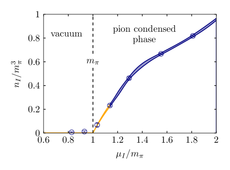
Figure 1: Phase transition between the vacuum and the pion condensed phase, as exhibited by the isospin density. The lattice data (blue points) are fitted using $\chi$PT (yellow curve) and matched to a spline interpolation (blue curve).

III Electroweak sector

We consider the scenario where the pion condensate is neutralized by a gas of charged leptons with mass $m_{\ell}$. In the present approach we assume leptons to be free relativistic particles. A systematic improvement over this assumption is possible by taking into account $\mathcal{O}(e^{2})$ electromagnetic effects perturbatively, both in the electroweak sector and in lattice QCD simulations. The lepton density $n_{\ell}$ is controlled by a lepton chemical potential $\mu_{\ell}$, from which the leptonic contribution to the pressure $p_{\ell}$ and to the energy density $\epsilon_{\ell}$ can be obtained, similarly to the QCD sector. We require local charge neutrality to hold, $n_{I}+n_{\ell}=0$, which uniquely determines the lepton chemical potential in terms of $\mu_{I}$. The corresponding EoS for electrons ($\ell=e$) and for muons ($\ell=\mu$) is also included in Fig. 2. We mention that this setup was also investigated in Ref. Andersen:2018nzq and a similar construction, assuming a first-order phase transition for pions, was discussed in Ref. Carignano:2016lxe .

In the vacuum phase, charged pions decay weakly into leptons, with a characteristic lifetime of $\tau_{\rm vac}\approx 10^{-8}\textmd{ s}$. In the condensed phase, the analogous weak process is quite different. Since the spontaneously broken symmetry group corresponds to the local gauge group of electromagnetism, the pion condensed phase is a superconductor, where the Goldstone mode is a linear combination of the electric charge eigenstates $\pi^{+}$ and $\pi^{-}$ Son:2000xc . In the presence of dynamical photons (in the unitary gauge) this mode disappears from the spectrum via the Higgs mechanism Migdal:1990vm , at the cost of a nonzero photon mass $m_{\gamma}\propto e|\sigma_{\pi}|$. In addition, the other linear combination of $\pi^{+}$ and $\pi^{-}$ develops a mass above $\mu_{I}$ Son:2000xc and is not excited if the temperature is sufficiently low. Thus, there is no light, electrically charged excitation that would decay weakly. However, besides condensation in the pseudoscalar channel, the ground state also exhibits an axial vector condensate $\sigma_{A}=\langle\bar{u}\gamma_{0}\gamma_{5}d+\bar{d}\gamma_{0}\gamma_{5}u\rangle/2$ that couples directly to the charged weak current as we discuss in Appendix C.

In Fig. 3 we show first lattice results for $\sigma_{A}$. The measurements at different values of the auxiliary pion source parameter are extrapolated to $\lambda\to 0$ using an approach similar to that of Ref. Brandt:2017oyy , employing a generalized Banks-Casher relation that we derive in Appendix A. Fig. 3 also includes the $\chi$PT prediction Brauner:2016lkh , for which we use $f_{\pi}$ as obtained above for the fit of $n_{I}$. The results clearly show $\sigma_{A}>0$ in the condensed phase and a nice agreement between the two approaches. The coupling of $\sigma_{A}$ to the weak current results in the depletion of the condensate and the production of charged antileptons and neutrinos. The characteristic lifetime $\tau$ of this process is calculated perturbatively in Appendix C. Normalized by the vacuum value $\tau_{\rm vac}$, we find that the lifetime takes the form

$$\mu_{I}>m_{\pi}:\quad\frac{\tau}{\tau_{\rm vac}}=\frac{\mu_{I}^{3}}{m_{\pi}^{3}}\left[\frac{1-m_{\ell}^{2}/m_{\pi}^{2}}{1-m_{\ell}^{2}/\mu_{I}^{2}}\right]^{2}\,,$$ (1)

where the $\chi$PT prediction for $\sigma_{A}$ was used.

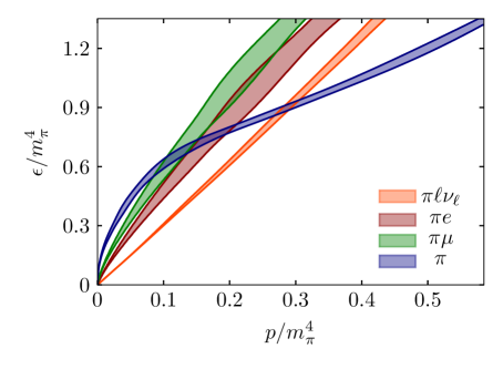
Figure 2: Equation of state in the pion condensed phase in the QCD sector and for the electrically neutral systems also including leptons (either muons or electrons) and neutrinos. The width of the curves incorporates statistical uncertainties as well as the uncertainty in the lattice pion mass for the pion-lepton systems.

Although suppressed deep in the condensed phase (as $\mu_{I}^{-3}$), weak decays therefore reduce the isospin charge of the system and create neutrinos $\nu_{\ell}$. For a high enough density of charged leptons and pions, the scattering cross section might be enhanced sufficiently to trap these neutrinos. Specifically, the conversion process $\nu_{\ell}\to\ell$ becomes possible where the neutrino couples to the condensate and transfers momentum to it. In addition, one also expects the cross section for $\nu_{\ell}\ell$ scattering to increase.

Thus, when the weak interactions are included, a consistent description of pion stars requires the inclusion of neutrinos. Therefore we consider the scenario where a gas of neutrinos – described by a density $n_{\nu_{\ell}}$ and a corresponding chemical potential $\mu_{\nu_{\ell}}$ – is also present in the system. At weak equilibrium, $\mu_{\nu_{\ell}}=\mu_{I}+\mu_{\ell}$, this setup can maintain a pion condensate for high neutrino density, as was already shown in Ref. Abuki:2009hx . In this case, neutrinos also contribute to the pressure and to the energy density by the amounts $p_{\nu_{\ell}}$ and $\epsilon_{\nu_{\ell}}$, respectively. Since there are two leptonic pion decay channels, we consider both electrons and muons, as well as their respective neutrinos in our calculations. Chemical equilibrium among the two families, resulting from neutrino oscillations, corresponds to $\mu_{\nu_{\mu}}=\mu_{\nu_{e}}$ or, equivalently, $\mu_{\mu}=\mu_{e}$. The EoS for this setup is also indicated in Fig. 2.

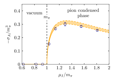
Figure 3: Lattice data for the axial vector condensate, extrapolated to vanishing pion source, $\lambda=0$, using our improvement program (blue points). The results are compared to the $\chi$PT prediction (yellow curve) Brauner:2016lkh .

IV Gravity sector

Using the resulting different equations of state, the mass $M$ and radius $R$ of pion stars can be computed by solving the Tolman-Oppenheimer-Volkoff (TOV) equations Tolman:1939jz ; Oppenheimer:1939ne , which describe hydrostatic equilibrium in general relativity, assuming spherical symmetry. Our implementation is detailed in Appendix B. Further stability analyses are performed by requiring the star to be robust against density perturbations glendenning2000compact and radial oscillations. The latter involves checking whether unstable modes exist by solving the corresponding Sturm-Liouville equation Bardeen . For more details on this analysis, see Appendix B. Fig. 4 shows the resulting mass-radius relations for pion stars of different compositions. The electrically charged pure pion stars have masses comparable to ordinary neutron stars, but an order of magnitude larger radii. The inclusion of leptons (either electrons or muons) increases both the masses and the radii considerably. Typically, the pion-electron configurations can be as heavy as intermediate-mass black holes Pasham:2015tca , whereas their radii are comparable to those of regular stars Torres:2009js .

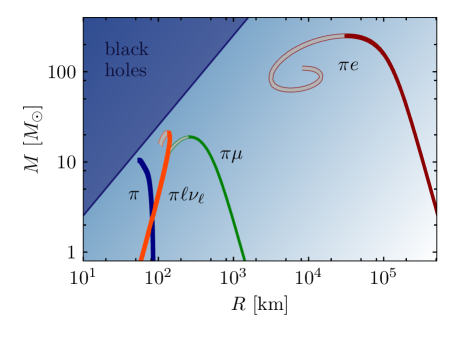
Figure 4: Mass-radius relations of various scenarios for pion stars. Shown is a pure pion star ($\pi$), a pion-electron ($\pi e$) and a pion-muon system ($\pi\mu$), together with a system containing both lepton families in chemical equilibrium ($\pi\ell\nu_{\ell}$). The filled (open) segments mark the gravitationally stable (unstable) solutions (for details see the text). The dark blue area marks the region excluded by causality and the background color represents the compactness $\beta\propto M/R$ of the objects (darker colors indicate more compact stars). The width of the curves indicates statistical errors and the uncertainty in the lattice pion mass.

In addition, we also considered a mixture of electrons and muons in chemical equilibrium by setting their respective chemical potentials equal. We observed that the gravitationally stable configurations for the latter setup cannot maintain a muonic component and are thus identical to those for the pion-electron system. Finally, the pion-lepton-neutrino scenario (with two lepton families in chemical equilibrium) again results in moderate masses and radii. We note that in this last case the star radius is defined by the point where the pressure of pions and of charged leptons vanishes, while $p_{\nu_{\ell}}$ is still nonzero. These configurations may therefore be viewed as a pion-lepton star in a neutrino cloud.

Such a cloud, in the form of a background of degenerate neutrinos could be present for a high leptochemical potential in the early universe, a possible cosmological scenario for temperatures below the QCD transition, as discussed in Ref. Wygas:2018otj . Astrophysical neutrino clouds (with massive neutrinos) in the form of a Fermi star would be stable on galactic scales, see e.g. Ref. Narain:2006kx . On the other hand, an unstable expanding neutrino cloud would lead to pion star configurations which are subject to evaporation near the border of the pion condensate. Consequently, the escaping neutrinos will continuously be replaced by the ones resulting from the decay of the condensate in the outer layers. The details of such an evaporation process will predominantly depend on the (density-dependent) pion lifetime, the neutrino mean free path and the radius of the star. This calculation is outside the scope of the present paper.

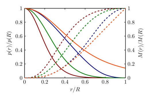
Figure 5: Integrated mass (dashed) and total pressure (solid) within the $\pi$ (blue), $\pi e$ (red), $\pi\mu$ (green), $\pi\ell\nu_{\ell}$ (orange) stars at their respective maximum mass, c.f. Fig. 4. The mass accumulates to its maximum value, whereas the pressure drops towards the boundary of the star. In the presence of neutrinos, a finite pressure remains at the boundary of the condensate region.

Table 1: Relevant properties of possible pion star compositions at their respective maximum mass. The last row correponds to the scenario with minimal neutrino pressure and $\mu_{\ell,c}/m_{\ell}$ is the relative electron chemical potential in this case.

	composition	$M^{\rm max}\,[M_{\odot}]$	$R^{\rm max}\,[\mathrm{km}]$	$\epsilon_{c}^{\rm max}\,[\mathrm{MeV\!/fm}^{3}]$	$p_{c}^{\rm max}\,[\mathrm{MeV\!/fm}^{3}]$	$\mu_{I,c}^{\rm max}/m_{\pi}-1$	$\mu_{\ell,c}^{\rm max}/m_{\ell}-1$
	$\pi$	10.5(5)	55(3)	57(5)	25(3)	1.068(4)	-
	$\pi e$	250(10)	$3.3(2)\times 10^{4}$	$4.5(4)\times 10^{-5}$	$3.5(4)\times 10^{-7}$	$5.59(2)\times 10^{-7}$	7.4(2)
	$\pi\mu$	18.9(4)	267(8)	2.7(3)	0.22(3)	$1.623(5)\times 10^{-2}$	0.58(3)
	$\pi\ell\nu_{\ell}|_{\mu_{\mu}=\mu_{e}}$	20.8(9)	137(6)	7.5(7)	2.3(2)	$4.13(2)\times 10^{-3}$	160(4)
	$\pi\ell\nu_{\ell}|_{\textmd{min.\ }p_{\nu_{\ell}}}$	28(2)	193(8)	3.7(4)	1.1(1)	$3.77(2)\times 10^{-3}$	155(4)

We point out that Fig. 4 reflects the $R\sim{\rm const.}$ behavior for pure pion stars (with masses below $7\,M_{\odot}$) – a telltale sign for an interaction-dominated EoS. The slope changes by the addition of leptons, scaling as $MR^{3}\sim{\rm const.}$, similarly to stars made of fermions. Having a non-vanishing pressure at the boundary from neutrinos leads to a $MR^{-3}\sim{\rm const.}$ behavior for the $\pi\ell\nu_{\ell}$ configuration, reminiscent of a self-bound star with constant density. Finally we also considered the $\pi\ell\nu_{\ell}$ system which minimizes the neutrino pressure at the star surface (and with it, the evaporation rate for the scenario of an expanding neutrino cloud). This condition was found to be met if $\mu_{\mu}=-m_{\mu}$ throughout the star. The corresponding results for $M(R)$ lie very close to the orange curve shown in Fig. 4 with somewhat higher masses and radii. The profiles for the pressure and for the integrated energy density of the maximal mass configurations are plotted in Fig. 5. Finally, an overview of the maximum masses and the corresponding radii is provided in Table. 1, together with the central values for the energy density $\epsilon_{c}$, the pressure $p_{c}$ and the chemical potentials $\mu_{I,c}$ and $\mu_{\ell,c}$.

V Conclusions

Pion stars provide a potential new class of compact objects, one that is made of a Bose-Einstein condensate of charged pions and a gas of leptons, being significantly different from neutron stars and white dwarfs both in their structure and gross features. Pion condensation might have occured in the early universe if large lepton asymmetries were present Schwarz:2009ii ; Abuki:2009hx ; Wygas:2018otj , serving as a primordial production mechanism for pion stars. These new compact objects might be revealed by the characteristic neutrino and photon spectra stemming from their evaporation or, if they survive sufficiently long, by signatures from companion stars via gravitational waves.

In the present paper we described the construction of pion stars and identified the key issues that concern their viability. There are open questions regarding the lifetime of pion stars, related to the question of weak stability, the possibility of neutrino trapping and the evaporation processes at the surface. The present analysis can be improved by addressing these issues in more detail and also by generalizing the calculation to nonzero temperatures, thereby making the contact to the potential primordial production mechanism more direct. Keeping these issues in mind, pion stars provide the first example in which the mass and radius of a compact stellar object can be determined from first principles. Furthermore, even if they happen to be short-lived, pion stars could constitute the first known case of a boson star and, remarkably, one with no need for any beyond Standard Model physics.

Acknowledgments E.S.F. and M.H. are partially supported by CNPq, FAPERJ and INCT-FNA Proc. No. 464898/2014-5. M.H. was also supported by FAPESP Proc. No. 2018/07833-1 and Capes Procs. No. 88887.185090/2018-00, via INCT-FNA, and 88881.133995/2016-01, which was determinant for his participation in this work. B.B.B., G.E. and S.S. acknowledge support from the DFG (EN 1064/2-1 and SFB/TRR 55). The authors are grateful to Jens O. Andersen and Misha Stephanov for inspiring discussions and useful comments. The authors also thank Oliver Witham for a careful reading of the manuscript, Alessandro Sciarra for help in creating the plots.

Appendix A Lattice setup and improvement

In the presence of the isospin chemical potential $\mu_{I}$ and the auxiliary pionic source parameter $\lambda$, the fermion matrices for the light and strange quarks read

$$M_{ud}=\not{D}(\mu_{I})+m_{ud}\mathds{1}+i\lambda\gamma_{5}\tau_{2}\,,\quad M_{s}=\not{D}(0)+m_{s}\,,$$ (2)

where $\not{D}$ is the Dirac operator,

$$\not{D}(\mu_{I})=\not{D}(0)\mathds{1}+\frac{\mu_{I}}{2}\gamma_{0}\tau_{3}\,,$$ (3)

$\tau_{a}$ denote the Pauli matrices acting in flavor space and $m_{ud}$ and $m_{s}$ are the light and strange quark masses, respectively. We discretize $\not{D}$ using the rooted staggered formulation, so that the Euclidean path integral over the gauge field $A_{\mu}$ becomes

$$\mathcal{Z}=\int\mathcal{D}A_{\mu}\,[\det M_{ud}]^{1/4}\,[\det M_{s}]^{1/4}\,e^{-S_{g}}\,,$$ (4)

where $S_{g}$ is the gluonic part of the QCD action, for which we use the tree level-improved Symanzik discretization. For the fermion matrices we employ stout smearing of the gauge fields. The determinants of $M_{ud}$ and of $M_{s}$ are positive Son:2000xc ; Kogut:2002zg , allowing for a probabilistic interpretation and standard Monte-Carlo algorithms. The quark masses are tuned to their physical values so that, in particular, $m_{\pi}\approx 135\textmd{ MeV}$ in the vacuum. The error of the pion mass used in the simulations originates primarily from the uncertainty of the lattice scale and amounts to $2\%$. Further details of our lattice action and our simulation algorithm are given in Refs. Aoki:2005vt ; Borsanyi:2010cj ; Endrodi:2014lja .

Here we perform simulations on a $24^{3}\times 32$ ensemble with lattice spacing $a\approx 0.29\textmd{ fm}$, a wide range of chemical potentials $0<\mu_{I}/m_{\pi}\leq 2$ and three pionic source parameters $0.17\leq\lambda/m_{ud}\leq 0.88$. The systematic uncertainties originating from lattice artefacts and from neglecting $\mathcal{O}(e^{2})$ electromagnetic effects will be investigated in a future publication. The volume of our system is around $7\textmd{ fm}^{3}$, sufficiently large so that finite size effects are under control. The temperature is significantly below the relevant QCD scales so that it well approximates $T=0$.

The isospin density and the pion condensate are obtained as derivatives of the partition function Brandt:2017oyy ,

$$n_{I} =\frac{1}{V_{4}}\frac{\partial\log\mathcal{Z}}{\partial\mu_{I}}=\frac{1}{2V_{4}}\left\langle\!\textmd{Re}\,\textmd{tr}\,\frac{[\not{D}(\mu_{I})+m_{ud}]^{\dagger}\not{D}^{\prime}\!(\mu_{I})}{|\not{D}(\mu_{I})+m_{ud}|^{2}+\lambda^{2}}\right\rangle\,,$$ (5)

$$\sigma_{\pi} =\frac{1}{V_{4}}\frac{\partial\log\mathcal{Z}}{\partial\lambda}=\frac{\lambda}{2V_{4}}\left\langle\textmd{tr}\,\frac{1}{|\not{D}(\mu_{I})+m_{ud}|^{2}+\lambda^{2}}\right\rangle\,,$$ (6)

where the prime denotes differentiation with respect to $\mu_{I}$. Similarly, the axial vector condensate reads

$$\sigma_{A}=\frac{\lambda}{2V_{4}}\left\langle\textmd{tr}\,\frac{U_{4}}{|\not{D}(\mu_{I})+m_{ud}|^{2}+\lambda^{2}}\right\rangle\,,$$ (7)

where $U_{4}$ is the staggered equivalent of the timelike component of the continuum axial vector operator Kilcup:1986dg that has also been used in Ref. Bali:2018sey . In Eqs. (5)–(7), $V_{4}=V/T$ is the four-dimensional volume of the system that includes the spatial volume $V=(N_{s}a)^{3}$ and the temperature $T=(N_{t}a)^{-1}$ in terms of the lattice spacing $a$ and the lattice geometry $N_{s}^{3}\times N_{t}$. Having measured the observables using different values of the pionic source parameter $\lambda$, the physical results are obtained via an extrapolation to $\lambda=0$. This is facilitated by using the singular value representation introduced in Ref. Brandt:2017oyy for the pion condensate, which we work out here for $\sigma_{A}$ as well.

Using the singular values $\xi_{n}$ of the massive Dirac operator,

$$|\not{D}(\mu_{I})+m_{ud}|^{2}\psi_{n}=\xi_{n}^{2}\psi_{n}\,,$$ (8)

the pion condensate is rewritten as

$$\begin{split}\sigma_{\pi}&=\frac{\lambda}{2V_{4}}\Big{\langle}\sum_{n}(\xi_{n}^{2}+\lambda^{2})^{-1}\Big{\rangle}\\ &\xrightarrow{V\to\infty}\frac{\lambda}{2}\Big{\langle}\int\!\textmd{d}\xi\,\rho(\xi)\,(\xi^{2}+\lambda^{2})^{-1}\Big{\rangle}\\ &\xrightarrow{\lambda\to 0}\frac{\pi}{4}\left\langle\rho(0)\right\rangle\,,\end{split}$$ (9)

where we performed the thermodynamic limit introducing the spectral density $\rho(\xi)$, followed by the $\lambda\to 0$ limit. This equation is the analogue of the Banks-Casher relation Banks:1979yr , connecting the order parameter of pion condensation to the density of singular values around the origin. The determination of $\rho(0)$ involves calculating the low singular values, building a histogram and fitting it to extract the spectral density at zero. In addition, a leading-order reweighting of the configurations to $\lambda=0$ is performed. For more details on our fitting strategy, see Ref. Brandt:2017oyy .

A very similar Banks-Casher-type relation can be found for $\sigma_{A}$ as well. The same steps as in Eq. (9) lead in this case to

$$\begin{split}\sigma_{A}&=\frac{\lambda}{2V_{4}}\Big{\langle}\!\sum_{n}(\xi_{n}^{2}+\lambda^{2})^{-1}\psi_{n}^{\dagger}U_{4}\psi_{n}\Big{\rangle}\\ &\xrightarrow{V\to\infty}\frac{\lambda}{2}\Big{\langle}\int\!\textmd{d}\xi\,\rho(\xi)\,(\xi^{2}+\lambda^{2})^{-1}\psi_{n}^{\dagger}U_{4}\psi_{n}\Big{\rangle}\\ &\xrightarrow{\lambda\to 0}\frac{\pi}{4}\big{\langle}\rho(0)\,\psi_{0}^{\dagger}U_{4}\psi_{0}\big{\rangle}.\end{split}$$ (10)

The matrix elements of $U_{4}$ are measured together with the singular values and extrapolated towards the low end of the spectrum to find $\psi_{0}^{\dagger}U_{4}\psi_{0}$. The so obtained results for $\sigma_{A}$ are shown in Fig. 3 of the body of the text.

We mention that the ratio of the axial vector condensate and the pion condensate can also be found from the axial Ward-identity. For $\mu_{I}\neq 0$ but $\lambda=0$, this operator identity reads

$$\partial_{\nu}\bar{\psi}\gamma_{\nu}\gamma_{5}\tau_{a}\psi=2m_{ud}\bar{\psi}\gamma_{5}\tau_{a}\psi+i\epsilon_{ab3}\,\mu_{I}\,\bar{\psi}\gamma_{0}\gamma_{5}\tau_{b}\psi\,.$$ (11)

Integrating in space and time, exploiting the periodic boundary conditions for the composite field $\bar{\psi}\psi$ in all directions and taking the expectation value over quarks and gluons we get for the $a=2$ component

$$\mu_{I}\sigma_{A}=-m_{ud}\sigma_{\pi}\,,$$ (12)

which is found to be satisfied within our statistical errors. (Notice that in our definitions $\sigma_{\pi}$ is related to $i\bar{\psi}\gamma_{5}\tau_{2}\psi$ and $\sigma_{A}$ to $\bar{\psi}\gamma_{0}\gamma_{5}\tau_{1}\psi/2$.)

Appendix B Equation of state and the TOV equations

In $\chi$PT the isospin density reads Son:2000xc ,

$$n_{I}=\frac{\mu_{I}f_{\pi}^{2}}{2}\left[1-\frac{m_{\pi}^{4}}{\mu_{I}^{4}}\right]\cdot\Theta(\mu_{I}-m_{\pi})\,,$$ (13)

where $f_{\pi}$ is the pion decay constant, which is the only parameter that we allow to vary for the $\chi$PT fit depicted in Fig. 1. For free relativistic leptons, the density is

$$n_{\ell}(\mu_{\ell})=\frac{1}{3\pi^{2}}(\mu_{\ell}^{2}-m_{\ell}^{2})^{3/2}\cdot\Theta(\mu_{\ell}-m_{\ell})\,.$$ (14)

The neutrino density $n_{\nu_{\ell}}(\mu_{\nu_{\ell}})$ is analogous to Eq. (14), just replacing the lepton mass $m_{\ell}$ by zero and dividing by a factor of 2 since only left-handed neutrinos are considered. The pionic pressure and energy density are calculated from $n_{I}(\mu_{I})$ at zero temperature via

$$p=\frac{\log\mathcal{Z}}{V_{4}}=\int_{0}^{\mu_{I}}\!\!\textmd{d}\mu_{I}^{\prime}\,n_{I}(\mu_{I}^{\prime}),\quad\quad\epsilon=-p+\mu_{I}n_{I}\,,$$ (15)

and similarly for the charged leptons and the neutrinos, using $n_{\ell}(\mu_{\ell})$ and $n_{\nu_{\ell}}(\mu_{\nu_{\ell}})$, respectively.

After requiring local charge neutrality $n_{\ell}=n_{I}$, the pion-lepton system is unambiguously characterized by the lepton chemical potential $\mu_{\ell}$. The total pressure $p$ and energy density $\epsilon$ enter the TOV equations Tolman:1939jz ; Oppenheimer:1939ne , which can be rewritten in terms of the chemical potentials as

$$\frac{\mathrm{d}\mu_{\ell}}{\mathrm{d}r}=-G\mu_{\ell}\,\frac{M+4\pi r^{3}p}{r^{2}-2rGM}\left[1+\frac{\mu_{I}}{\mu_{\ell}}\right]\left[1+\frac{n_{\ell}^{\prime}}{n_{I}^{\prime}}\right]^{-1},$$ (16)

where $G$ is Newton’s constant, the primes denote derivatives with respect to the corresponding chemical potentials, we used natural units $c=\hbar=1$ and

$$M(r)=4\pi\int_{0}^{r}\!\mathrm{d}r^{\prime}\,r^{\prime 2}\epsilon(r^{\prime}),$$ (17)

is the integrated mass. Eqs. (16)-(17) remain unchanged if neutrinos are included in the EoS, only $p$ and $\epsilon$ need to be complemented by the respective neutrino contributions. The first TOV equation (16) for two lepton families ($\ell=e,\mu$) takes the form

$$\frac{\mathrm{d}\mu_{e}}{\mathrm{d}r} =-G\mu_{e}\frac{M+4\pi r^{3}p}{r^{2}-2rGM}$$ (18)

$$\phantom{=}~{}\cdot\left[1+\frac{\mu_{I}}{\mu_{e}}+\rho\left(\frac{\mu_{\mu}}{\mu_{e}}-1\right)\right]$$

$$\phantom{=}~{}\cdot\left[1+\frac{n_{e}^{\prime}}{n_{I}^{\prime}}+\frac{n_{\mu}^{\prime}}{n_{I}^{\prime}}\frac{\mathrm{d}\mu_{\mu}}{\mathrm{d}\mu_{e}}+\rho\left(\frac{\mathrm{d}\mu_{\mu}}{\mathrm{d}\mu_{e}}-1\right)\right]^{-1},$$

with asymmetry $\rho=(n_{\mu}+n_{\nu_{\mu}})/(n_{e}+n_{\nu_{e}}+n_{\mu}+n_{\nu_{\mu}})$ between the lepton families. Note that for $\mu_{\mu}=\mu_{e}$ or $\rho=0$ the last terms in both square brackets vanish.

The TOV equations are integrated numerically up to the star boundary $r=R$, where $p_{\pi}+p_{\ell}$ vanishes and the total mass $M=M(R)$ is attained. Note that for pion-lepton-neutrino configurations, the neutrino pressure is nonzero at the so defined boundary. The points of the mass-radius curves in Fig. 4 correspond to different values of the central energy density $\epsilon_{c}$.

The gravitational stability of the solutions is investigated by looking at unstable radial modes. In particular, we integrate the Sturm-Liouville equation with oscillation frequency $\omega=0$ and check whether the resulting oscillation amplitude has nodepoints within the star. If so, then there exists at least one frequency $\omega^{2}<0$, driving the system unstable on long timescales Bardeen . In the $\pi\ell\nu_{\ell}$ case, the integration of the Sturm-Liouville equation was only performed up to the boundary of the pion condensate. Nevertheless, this was sufficient to observe whether there are unstable modes (nodepoint within the pion condensate), or indications of it (no nodepoint, but a clear tendency for it within the surrounding neutrino cloud). This approach ruled out some configurations that seemed stable according to the necessary (but not sufficient) condition glendenning2000compact , $\textmd{d}M\!(R)/\textmd{d}\epsilon_{c}>0$.

Appendix C Weak decay in the condensed phase

As discussed in Sec. III, the condensed phase exhibits massive photons and no light charged pionic degrees of freedom. Thus, standard approaches involving the weak decay of a momentum eigenstate pion do not apply. Instead, we need to consider the production of a lepton pair $\ell(\mathbf{k})\nu_{\ell}(\mathbf{q})$ out of the condensed ground state $\Omega$, where $\mathbf{k}$ and $\mathbf{q}$ denote the momenta of the charged antilepton and of the neutrino, respectively. As mentioned in Sec. III, if neutrinos are trapped and the weak equilibrium condition $\mu_{\nu_{\ell}}=\mu_{I}+\mu_{\ell}$ is satisfied, the decay at zero temperature is Pauli-blocked since all final lepton states are filled.

For completeness, here we consider the situation, where neutrinos are absent and all final lepton states are available. According to Fermi’s golden rule, the differential probability for the decay process is related to the $S$-matrix element schwartz2014quantum

$$\textmd{d}P=\sum_{s_{\ell},s_{\nu_{\ell}}}\frac{|\langle\Omega\ell\nu_{\ell}|S|\Omega\rangle|^{2}}{\langle\Omega|\Omega\rangle^{2}\langle\ell|\ell\rangle\langle\nu_{\ell}|\nu_{\ell}\rangle}\,\left[\frac{V}{(2\pi)^{3}}\right]^{2}\textmd{d}^{3}\mathbf{k}\,\textmd{d}^{3}\mathbf{q}\,,$$ (19)

involving a sum over the spins $s_{\ell}$ and $s_{\nu_{\ell}}$ of the outgoing leptons. For regularization purposes we need to assume that the decay proceeds in a finite volume $V$ and over a finite time interval $\mathcal{T}$.

The ground state has unit norm, $\langle\Omega|\Omega\rangle=1$, while the normalization of the lepton states takes the usual form,

$$\langle\ell|\ell\rangle=2E_{\ell}V,\quad\quad\langle\nu_{\ell}|\nu_{\ell}\rangle=2E_{\nu_{\ell}}V\,,$$ (20)

where the leptons are on shell,

$$E_{\ell}=\sqrt{\mathbf{k}^{2}+m_{\ell}^{2}},\quad\quad E_{\nu_{\ell}}=|\mathbf{q}|\,.$$ (21)

The $S$-matrix element factorizes into leptonic and hadronic parts,

$$\begin{split}\langle\Omega\ell&\nu_{\ell}|S|\Omega\rangle=\frac{G_{\rm F}\cos\vartheta_{c}}{\sqrt{2}}\\ &\;\cdot\langle\ell\nu_{\ell}|\bar{\ell}\gamma^{\mu}(1-\gamma_{5})\nu_{\ell}|0\rangle\cdot\langle\Omega|\bar{u}\gamma_{\mu}(1-\gamma_{5})d|\Omega\rangle\,,\end{split}$$ (22)

where $G_{\rm F}$ is the Fermi constant and $\vartheta_{c}$ the Cabibbo angle. The leptonic component can be treated as usual okun2013leptons . The hadronic factor reflects the accumulation of weak vertices in the pion condensate. While the expectation value of the vector part vanishes, $\left\langle\Omega|\bar{u}\gamma_{\mu}d|\Omega\right\rangle=0$, the zeroth component of the axial vector part is nonzero. In $\chi$PT it reads Brauner:2016lkh

$$\langle\Omega|\bar{u}\gamma_{0}\gamma_{5}d|\Omega\rangle=\sigma_{A}=-\frac{m_{\pi}^{2}f_{\pi}^{2}}{2\mu_{I}}\sqrt{1-\frac{m_{\pi}^{4}}{\mu_{I}^{4}}}\cdot\Theta(\mu_{I}-m_{\pi})\,,$$ (23)

which is plotted in Fig. 3 together with the corresponding lattice data.

Energy conservation implies $\mu_{I}=E_{\ell}+E_{\nu_{\ell}}$, since after the decay the charge of the condensate is reduced by one unit, releasing $\mu_{I}$ energy. To maintain the zero-momentum state of $\Omega$, we assume that the condensate picks up zero momentum so that momentum conservation fixes $\mathbf{k}=-\mathbf{q}$. Performing the spin sums in the leptonic factor, the squared matrix element for $\mu_{I}>m_{\pi}$ becomes

$$\begin{split}\sum_{s_{\ell},s_{\nu_{\ell}}}\!|\langle\Omega\ell&\nu_{\ell}|S|\Omega\rangle|^{2}\!=4\,G_{\rm F}^{2}\cos^{2}\!\vartheta_{c}\,\sigma_{A}^{2}\,(E_{\ell}E_{\nu_{\ell}}+\mathbf{k}\cdot\mathbf{q})\\ &\cdot(2\pi)^{4}\delta(\mu_{I}-E_{\ell}-E_{\nu_{\ell}})\,\delta^{(3)}(\mathbf{k}+\mathbf{q})\,V\mathcal{T}\,,\end{split}$$ (24)

where the regularization $(2\pi)^{4}\,\delta(0)\,\delta^{(3)}(\mathbf{0})=V\mathcal{T}$ was used.

Inserting this in Eq. (19), performing the integrals over the momenta and using the on-shell conditions (21), the decay rate $\Gamma=\int\!\textmd{d}P/\,\mathcal{T}$ in the condensed phase $\mu_{I}>m_{\pi}$ reads

$$\Gamma=\Gamma_{\rm vac}\cdot\frac{m_{\pi}^{3}}{\mu_{I}^{3}}\left[\frac{1-m_{\ell}^{2}/\mu_{I}^{2}}{1-m_{\ell}^{2}/m_{\pi}^{2}}\right]^{2}\!\cdot n_{Q}V\,,$$ (25)

where $\Gamma_{\rm vac}$ is the decay rate of a pion at rest in the vacuum (see, e.g., Ref. okun2013leptons ) and we factored out the density $n_{Q}=n_{I}$ using Eq. (13). Thus, for high isospin chemical potentials, $\Gamma$ is reduced as $\mu_{I}^{-3}$. The result (25) is extensive in the volume, since the weak current can couple to the condensate at any point in space. Keeping the number of charges $N_{Q}=n_{Q}V$ fixed, in the limit $\mu_{I}\to m_{\pi}$ the decay rate reproduces $N_{Q}$ times the vacuum decay rate, satisfying continuity of $\Gamma$ at the pion condensation onset. Altogether, the average lifetime of the condensate thus reads $\tau=(\Gamma/N_{Q})^{-1}$, giving Eq. (1) in the body of the text.

References

- (1) Virgo, LIGO Scientific Collaboration, Abbott, B. P. et al., “GW170817: Observation of Gravitational Waves from a Binary Neutron Star Inspiral,” Phys. Rev. Lett. 119 (2017) 161101, arXiv:1710.05832 [gr-qc].
- (2) Landau, L. D., “On the theory of stars,” Physik. Zeits. Sowjetunion 1 (1932) 285.
- (3) Baade, W. and Zwicky, F., “On super-novae,” Proc. Nat. Acad. Sci. U.S. 20 (1934) 254.
- (4) Hewish, A., Bell, S. J., Pilkington, J. D. H., Scott, P. F., and Collins, R. A., “Observation of a rapidly pulsating radio source,” Nature 217 (1968) 709–713.
- (5) Son, D. T. and Stephanov, M. A., “QCD at finite isospin density,” Phys. Rev. Lett. 86 (2001) 592–595, arXiv:hep-ph/0005225 [hep-ph].
- (6) Wheeler, J. A., “Geons,” Phys. Rev. 97 (1955) 511–536.
- (7) Kaup, D. J., “Klein-Gordon Geon,” Phys. Rev. 172 (1968) 1331–1342.
- (8) Jetzer, P., “Boson stars,” Phys. Rept. 220 (1992) 163–227.
- (9) Colpi, M., Shapiro, S. L., and Wasserman, I., “Boson Stars: Gravitational Equilibria of Selfinteracting Scalar Fields,” Phys. Rev. Lett. 57 (1986) 2485–2488.
- (10) Coleman, S. R., “Q Balls,” Nucl. Phys. B262 (1985) 263. [Erratum: Nucl. Phys.B269,744(1986)].
- (11) Alford, M. G., “Q Clouds,” Nucl. Phys. B298 (1988) 323–332.
- (12) Liebling, S. L. and Palenzuela, C., “Dynamical Boson Stars,” Living Rev. Rel. 15 (2012) 6, arXiv:1202.5809 [gr-qc].
- (13) Migdal, A. B., Chernoutsan, A. I., and Mishustin, I. N., “Pion condensation and dynamics of neutron stars,” Phys. Lett. 83B (1979) 158–160.
- (14) L. Vartanian, Y., Hajyan, G., and Alaverdyan, G., “Pion stars,”.
- (15) Migdal, A. B., Saperstein, E. E., Troitsky, M. A., and Voskresensky, D. N., “Pion degrees of freedom in nuclear matter,” Phys. Rept. 192 (1990) 179–437.
- (16) Schwarz, D. J. and Stuke, M., “Lepton asymmetry and the cosmic QCD transition,” JCAP 0911 (2009) 025, arXiv:0906.3434 [hep-ph]. [Erratum: JCAP1010,E01(2010)].
- (17) Abuki, H., Brauner, T., and Warringa, H. J., “Pion condensation in a dense neutrino gas,” Eur. Phys. J. C64 (2009) 123–131, arXiv:0901.2477 [hep-ph].
- (18) Wygas, M. M., Oldengott, I. M., Bodeker, D., and Schwarz, D. J., “The cosmic QCD epoch at non-vanishing lepton asymmetry,” arXiv:1807.10815 [hep-ph].
- (19) Brandt, B. B., Endrődi, G., and Schmalzbauer, S., “QCD phase diagram for nonzero isospin-asymmetry,” Phys. Rev. D97 no. 5, (2018) 054514, arXiv:1712.08190 [hep-lat].
- (20) Endrődi, G., “Magnetic structure of isospin-asymmetric QCD matter in neutron stars,” Phys. Rev. D90 (2014) 094501, arXiv:1407.1216 [hep-lat].
- (21) Brandt, B. B., Endrődi, G., and Schmalzbauer, S., “QCD at finite isospin chemical potential,” in 35th International Symposium on Lattice Field Theory (Lattice 2017). 2017. arXiv:1709.10487 [hep-lat].
- (22) Kogut, J. B. and Sinclair, D. K., “Lattice QCD at finite isospin density at zero and finite temperature,” Phys. Rev. D66 (2002) 034505, arXiv:hep-lat/0202028 [hep-lat].
- (23) Andersen, J. O. and Kneschke, P., “Bose-Einstein condensation and pion stars,” arXiv:1807.08951 [hep-ph].
- (24) Carignano, S., Lepori, L., Mammarella, A., Mannarelli, M., and Pagliaroli, G., “Scrutinizing the pion condensed phase,” Eur. Phys. J. A53 (2017) 35, arXiv:1610.06097 [hep-ph].
- (25) Brauner, T. and Huang, X.-G., “Vector meson condensation in a pion superfluid,” Phys. Rev. D94 no. 9, (2016) 094003, arXiv:1610.00426 [hep-ph].
- (26) Tolman, R. C., “Static solutions of Einstein’s field equations for spheres of fluid,” Phys. Rev. 55 (1939) 364–373.
- (27) Oppenheimer, J. R. and Volkoff, G. M., “On Massive neutron cores,” Phys. Rev. 55 (1939) 374–381.
- (28) Glendenning, N., Compact Stars: Nuclear Physics, Particle Physics, and General Relativity. Astronomy and Astrophysics Library. Springer New York, 2000.
- (29) Bardeen, J. M., Thorne, K. S., and Meltzer, D. W., “A Catalogue of Methods for Studying the Normal Modes of Radial Pulsation of General-Relativistic Stellar Models,” Astrophysical Journal 145 (1966) 505.
- (30) Pasham, D. R., Strohmayer, T. E., and Mushotzky, R. F., “A 400 solar mass black hole in the Ultraluminous X-ray source M82 X-1 accreting close to its Eddington limit,” Nature 513 (2015) 74–76, arXiv:1501.03180 [astro-ph.HE].
- (31) Torres, G., Andersen, J., and Gimenez, A., “Accurate masses and radii of normal stars: modern results and applications,” Astron. Astrophys. Rev. 18 (2010) 67–126, arXiv:0908.2624 [astro-ph.SR].
- (32) Narain, G., Schaffner-Bielich, J., and Mishustin, I. N., “Compact stars made of fermionic dark matter,” Phys. Rev. D74 (2006) 063003, arXiv:astro-ph/0605724 [astro-ph].
- (33) Aoki, Y., Fodor, Z., Katz, S. D., and Szabó, K. K., “The Equation of state in lattice QCD: With physical quark masses towards the continuum limit,” JHEP 01 (2006) 089, arXiv:hep-lat/0510084 [hep-lat].
- (34) Borsányi, S. et al., “The QCD equation of state with dynamical quarks,” JHEP 11 (2010) 077, arXiv:1007.2580 [hep-lat].
- (35) Kilcup, G. W. and Sharpe, S. R., “A Tool Kit for Staggered Fermions,” Nucl. Phys. B283 (1987) 493–550.
- (36) Bali, G. S., Brandt, B. B., Endrődi, G., and Gläßle, B., “Weak decay of magnetized pions,” arXiv:1805.10971 [hep-lat].
- (37) Banks, T. and Casher, A., “Chiral Symmetry Breaking in Confining Theories,” Nucl. Phys. B169 (1980) 103–125.
- (38) Schwartz, M., Quantum Field Theory and the Standard Model. Cambridge University Press, 2014.
- (39) Okun, L., Leptons and Quarks. North-Holland Personal Library. Elsevier Science, 2013.