Frequency-Selective Hybrid Beamforming Based on Implicit CSI for Millimeter Wave Systems

Abstract

Hybrid beamforming is a promising concept to achieve high data rate transmission at millimeter waves. To implement it in a transceiver, many references optimally adapt to a high-dimensional multi-antenna channel but more or less ignore the complexity of the channel estimation. Realizing that received coupling coefficients of the channel and pairs of possible analog beamforming vectors can be used for analog beam selection, we further propose a low-complexity scheme that exploits the coupling coefficients to implement hybrid beamforming. Essentially, the coupling coefficients can be regarded as implicit channel state information (CSI), and the estimates of these coupling coefficients yield alternatives of effective channel matrices of much lower dimension. After calculating the Frobenius norm of these effective channel matrices, it turns out that the effective channel having the largest value of the Frobenius norm provides the solution to hybrid beamforming problem.

I Introduction

With the rapid increase of data rates in wireless communications, bandwidth shortage is getting more critical. Therefore, there is a growing interest in using millimeter wave (mmWave) for future wireless communications taking advantage of the enormous amount of available spectrum [1]. When systems operate at mmWave frequency bands, a combination of analog beamforming [2, 3] and digital beamforming [4] can be one of the low-cost solutions, which is commonly called hybrid beamforming [5]-[8]. Unquestionably, it is intractable to deal with hybrid beamforming at a transmitter and a receiver simultaneously because there are four unknown matrices (two analog and two digital beamforming matrices). To avoid dealing with all these issues at the same time, one can simplify the problem by initially assuming that the channel matrix is known. Then the problem of hybrid beamforming on both sides (i.e., finding the precoder and combiner) can be solved by utilizing the singular value decomposition (SVD) of the channel matrix [5]-[8]. Unfortunately, the overhead of some preliminary work, such as channel estimation for large-scale antenna arrays [9, 10], makes the previously proposed solutions difficult to obtain.

Our previous work in [11] explains that the analog beam selection based on the power estimates is equivalent to the beam selection by the orthogonal matching pursuit (OMP) algorithm [12] when the analog beamforming vectors are selected from orthogonal codebooks. However, the result of the analog beam selection technique based on the received power can be further improved because the factor dominating the performance of hybrid beamforming is the singular values of the effective channel $\mathbf{H}_{E}$ rather than the received power. A simple cure for the problem is that one can reserve a few more candidates of the analog beamforming vectors associated with the large received power levels. Then, the subset of these candidates yielding maximum throughput will provide the optimal solution to the hybrid beamforming. Again it is evident that the computational complexity exponentially increases as the size of the enlarged candidate set. Consequently, we have a strong motivation to find a relationship between the observations for the analog beam selection and a key parameter of the hybrid beamforming gain, and then use the relationship to facilitate the analog beam selection and the corresponding optimal digital beamforming. In the low SNR regime, we find that the Frobenius norm of $\mathbf{H}_{E}$ is the key parameter of the hybrid beamforming gain. Moreover, the observations for the analog beam selection can be used to generate $\mathbf{H}_{E}$. Accordingly, the collected observations yielding the maximum value of the key parameter gives us the necessary information to optimally select the analog as well as the corresponding digital beamforming matrices.

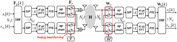
Figure 1: A transceiver has hybrid analog-digital beamforming structures on both sides, where DBF is short for digital beamforming. Each analog beamforming vector has multiple phase shifters connecting to one RF chain, which includes a digital-to-analog converter (DAC) at the transmitter or an analog-to-digital converter (ADC) at the receiver.

We use the following notations throughout this paper. $a$ is a scalar, $\mathbf{a}$ is a column vector, and $\mathbf{A}$ is a matrix. $\mathbf{a}_{n}$ denotes the $n^{\text{th}}$ column vector of $\mathbf{A}$; $\left[\mathbf{A}\right]_{n,n}$ denotes the $n^{\text{th}}$ diagonal element of $\mathbf{A}$; $\left[\mathbf{A}\right]_{:,1:N}$ denotes the first $N$ column vectors of $\mathbf{A}$; $\left[\mathbf{A}\right]_{1:N,1:N}$ denotes the $N\times N$ submatrix extracted from the upper-left corner of $\mathbf{A}$. $\mathbf{A}^{*}$, $\mathbf{A}^{H}$, and $\mathbf{A}^{T}$ denote the complex conjugate, Hermitian transpose and transpose of $\mathbf{A}$. $\left\|\mathbf{A}\right\|_{F}$ denotes the Frobenius norm of $\mathbf{A}$. $\mathbf{I}_{N}$ and $\mathbf{0}_{N\times M}$ denote the $N\times N$ identity and $N\times M$ zero matrices.

II System Model

A system having a transmitter with an $N_{T}$-element uniform linear antenna array (ULA) communicate $N_{S}$ OFDM data streams to a receiver with an $N_{R}$-element ULA as shown in Fig. 1. At the transmitter, a precoder $\mathbf{F}_{P}\mathbf{F}_{B}[k]$ at each subcarrier $k=1,\cdots,K$ includes a analog beamforming matrix $\mathbf{F}_{P}\in\mathbb{C}^{N_{T}\times N_{RF}}$ and a digital beamforming matrix $\mathbf{F}_{B}[k]\in\mathbb{C}^{N_{RF}\times N_{S}}$. The $N_{RF}$ analog beamforming vectors in matrix $\mathbf{F}_{P}$ are selected from a predefined codebook $\mathcal{F}=\{\tilde{\mathbf{f}}_{n_{f}}\in\mathbb{C}^{N_{T}\times 1},n_{f}=1,\cdots,N_{F}\}$ with the $n_{f}^{\text{th}}$ member represented as [3]

$$\tilde{\mathbf{f}}_{n_{f}}=\frac{1}{\sqrt{N_{T}}}\left[1,e^{j\frac{2\pi}{\lambda_{0}}\text{sin}(\phi_{T,n_{f}})\Delta_{d}},\cdots,e^{j\frac{2\pi}{\lambda_{0}}\text{sin}(\phi_{T,n_{f}})\cdot(N_{T}-1)\Delta_{d}}\right]^{T},$$ (1)

where $\phi_{T,n_{f}}$ stands for the $n_{f}^{\text{th}}$ candidate of the steering angles at the transmitter, $\Delta_{d}=\lambda_{0}/2$ is the distance between two neighboring antennas, and $\lambda_{0}$ is the wavelength at the carrier frequency. At the receiver, the combiner $\mathbf{W}_{P}\mathbf{W}_{B}[k]$ has a similar structure as the precoder: $\mathbf{W}_{P}\in\mathbb{C}^{N_{R}\times N_{RF}}$ and $\mathbf{W}_{B}[k]\in\mathbb{C}^{N_{RF}\times N_{S}}$ are the analog and digital beamforming matrices, respectively. Also, the columns of $\mathbf{W}_{P}$ are selected from the other codebook $\mathcal{W}=\{\tilde{\mathbf{w}}_{n_{w}}\in\mathbb{C}^{N_{R}\times 1},n_{w}=1,\cdots,N_{W}\}$, where the members can be generated by the same rule as (1). Due to hardware constraints, the analog beamforming matrices are constant within one OFDM symbol duration.

Via a coupling of the precoder, combiner, and a frequency-selective fading channel $\mathbf{H}[k]\in\mathbb{C}^{N_{R}\times N_{T}}$, the received signal $\mathbf{r}[k]\in\mathbb{C}^{N_{S}\times 1}$ at subcarrier $k$ can be written as

$$\mathbf{r}[k] =\sqrt{\rho}\cdot\mathbf{W}_{B}^{H}[k]\mathbf{W}_{P}^{H}\mathbf{H}[k]\underset{\mathbf{x}[k]}{\underbrace{\mathbf{F}_{P}\mathbf{F}_{B}[k]\mathbf{s}[k]}}+\underset{\mathbf{z}[k]}{\underbrace{\mathbf{W}_{B}^{H}[k]\mathbf{W}_{P}^{H}\mathbf{n}[k]}}$$ (2)

$$=\sqrt{\rho}\cdot\mathbf{W}_{B}^{H}[k]\mathbf{W}_{P}^{H}\mathbf{H}[k]\mathbf{x}[k]+\mathbf{z}[k],$$

where $\rho$ stands for the average received power including the transmit power, transmit antenna gain, receive antenna gain, and path loss, $\mathbf{s}[k]\in\mathbb{C}^{N_{S}\times 1}$ is the transmitted pilot or data vector whose covariance matrix $\mathbf{R}_{s}=\text{E}[\mathbf{s}[k]\mathbf{s}^{H}[k]]$ is a diagonal matrix, and $\mathbf{n}[k]\in\mathbb{C}^{N_{R}\times 1}$ is an $N_{R}$-dimensional independent and identically distributed (i.i.d.) complex Gaussian random vector, i.e., $\mathbf{n}[k]\sim\mathcal{CN}(\boldsymbol{0}_{N_{R}\times 1},\sigma_{n}^{2}\mathbf{I}_{N_{R}})$. Furthermore, the precoded transmitted signal $\mathbf{x}[k]$ and combined noise vector $\mathbf{z}[k]$ are enforced to satisfy the following two conditions: constant transmit power at each subcarrier and that the combined noise vector $\mathbf{z}[k]$ remains i.i.d.,

$$\begin{cases}\text{tr}(\mathbf{R}_{x})=\text{tr}\left(\mathbf{F}_{P}\mathbf{F}_{B}[k]\mathbf{R}_{s}\mathbf{F}_{B}^{H}[k]\mathbf{F}_{P}^{H}\right)=\text{tr}(\mathbf{R}_{s}),\\ \mathbf{R}_{z}=\sigma_{n}^{2}\mathbf{W}_{B}^{H}[k]\mathbf{W}_{P}^{H}\mathbf{W}_{P}\mathbf{W}_{B}[k]=\sigma_{n}^{2}\mathbf{I}_{N_{S}},\end{cases}$$ (3)

which can also be regarded as power constraints on the precoder and combiner.

The properties of mmWave channels have been widely studied recently [13, 14]. Based on the references, a simplified cluster-based frequency-selective fading channel has $C$ clusters and $R$ rays of each cluster. At subcarrier $k$, the channel matrix can be written as

$$\begin{aligned} \mathbf{H}[k]&=\sum_{c=1}^{C}\sum_{r=1}^{R}\alpha_{c,r}\cdot e^{-j2\pi kl_{c,r}/K}\cdot\mathbf{a}_{A}(\phi_{A,c,r})\mathbf{a}_{D}(\phi_{D,c,r})^{H}\end{aligned},$$ (4)

where the channel characteristics are given by the following parameters: $\alpha_{c,r}\in\mathbb{R}_{>0}$ describes the inter- and intra-cluster power and $\sum_{c=1}^{C}\sum_{r=1}^{R}|\alpha_{c,r}|^{2}=1$. $l_{c,r}\in\mathbb{R}_{\geq 0}$ stands for the delay index measured in unit of the sampling interval. Intra-cluster angle of departure (AoD) $\begin{aligned} \phi_{D,c,r}&=\phi_{D,c}+c_{D}\Delta_{r}\end{aligned}$, where the mean $\phi_{D,c}\sim\mathcal{U}(-\tfrac{\pi}{2},\tfrac{\pi}{2})$, and the other two factors (the angle spread $c_{D}$ and the offset angle $\Delta_{r}$) are given in [14] Table 7.5-3 and Table 7.5-6. In the same way, one can generate intra-cluster angle of arrival (AoA) $\phi_{A,c,r}$. The departure array response vector $\mathbf{a}_{D}(\phi_{D,c,r})$ has entries of equal magnitude and is a function of AoD represented as

$$\mathbf{a}_{D}(\phi_{D,c,r})=\frac{1}{\sqrt{N_{T}}}\left[1,e^{j\tfrac{2\pi}{\lambda_{0}}\text{sin}(\phi_{D,c,r})\Delta_{d}},\cdots,\right.\\ \left.e^{j\tfrac{2\pi}{\lambda_{0}}\text{sin}(\phi_{D,c,r})(N_{T}-1)\Delta_{d}}\right]^{T},$$ (5)

and the arrival array response vector $\mathbf{a}_{A}(\phi_{A,c,r})$ has a similar form as (5).

III Problem Statement

The objective of the precoder $\mathbf{F}_{P}\mathbf{F}_{B}[k]\,\forall k$ and the associated combiner $\mathbf{W}_{P}\mathbf{W}_{B}[k]\,\forall k$ is to achieve the maximum throughput across all subcarriers subject to the power constraints. That is, we seek matrices that solve

$$\begin{gathered}\begin{gathered}{\displaystyle\underset{\mathbf{F}_{P},\mathbf{W}_{P},(\mathbf{F}_{B}[k],\mathbf{W}_{B}[k])\,\forall k}{\max}}\,\sum_{k=0}^{K-1}I(\mathbf{F}_{P},\mathbf{W}_{P},\mathbf{F}_{B}[k],\mathbf{W}_{B}[k]),\end{gathered}\\ \text{s.t. }\begin{cases}\mathbf{f}_{P,n_{rf}}\in\mathcal{F},\mathbf{w}_{P,n_{rf}}\in\mathcal{W}\>\>\forall n_{rf},\\ \text{tr}\left(\mathbf{F}_{P}\mathbf{F}_{B}[k]\mathbf{R}_{s}\mathbf{F}_{B}^{H}[k]\mathbf{F}_{P}^{H}\right)=\text{tr}(\mathbf{R}_{s})\,\forall k,\\ \mathbf{W}_{B}^{H}[k]\mathbf{W}_{P}^{H}\mathbf{W}_{P}\mathbf{W}_{B}[k]=\mathbf{I}_{N_{S}}\,\forall k,\end{cases}\end{gathered}$$ (6)

where $\mathbf{f}_{P,n_{rf}}$ and $\mathbf{w}_{P,n_{rf}}$ are respectively the $n_{rf}^{\text{th}}$ column vectors of $\mathbf{F}_{P}$ and $\mathbf{W}_{P}$. The last two constraints are the consequences of (3) and the throughput at subcarrier $k$ is defined as [6]

$$I(\mathbf{F}_{P},\mathbf{W}_{P},\mathbf{F}_{B}[k],\mathbf{W}_{B}[k])=\\ \log_{2}\det\left(\mathbf{I}_{N_{S}}+\rho\mathbf{R}_{z}^{-1}\left(\mathbf{W}_{B}^{H}[k]\mathbf{W}_{P}^{H}\mathbf{H}[k]\mathbf{F}_{P}\mathbf{F}_{B}[k]\right)\right.\\ \left.\cdot\,\mathbf{R}_{s}\left(\mathbf{W}_{B}^{H}[k]\mathbf{W}_{P}^{H}\mathbf{H}[k]\mathbf{F}_{P}\mathbf{F}_{B}[k]\right)^{H}\right).$$ (7)

The solution to (6) is denoted as $(\mathbf{F}_{P,Opt},\mathbf{W}_{P,Opt},(\mathbf{F}_{B,Opt}[k],\mathbf{W}_{B,Opt}[k])\,\forall k)$.

If explicit channel state information (CSI), $\mathbf{H}[k]$, $k=0,\cdots,K-1$, is available, the problem of the precoder and combiner can be solved according to the references [5, 6]. In this paper, we consider a more pragmatic approach that channel knowledge is neither given nor estimated. To efficiently get the solution to (6), we try an alternative expression of (6) which has less probability to obtain the optimal solution as follows: given two sets $\mathcal{I_{F}}$ and $\mathcal{I_{W}}$ containing the candidates of $\mathbf{F}_{P}$ and $\mathbf{W}_{P}$, the achievable data rate in (6) is greater than or equal to

$$\begin{gathered}{\displaystyle\underset{\scriptsize\begin{array}[]{c}\mathbf{F}_{P}\in\mathcal{I_{F}}\\ \mathbf{W}_{P}\in\mathcal{I_{W}}\end{array}}{\max}}\underset{I_{LM}(\mathbf{F}_{P},\mathbf{W}_{P}):\text{ local maximum throughput}}{\underbrace{\left\{\begin{gathered}\max_{(\mathbf{F}_{B}[k],\mathbf{W}_{B}[k])\,\forall k}\,\sum_{k=0}^{K-1}I(\mathbf{F}_{P},\mathbf{W}_{P},\mathbf{F}_{B}[k],\mathbf{W}_{B}[k])\\ \text{s.t. }\begin{cases}\text{tr}\left(\mathbf{F}_{P}\mathbf{F}_{B}[k]\mathbf{R}_{s}\mathbf{F}_{B}^{H}[k]\mathbf{F}_{P}^{H}\right)=\text{tr}(\mathbf{R}_{s})\,\forall k\\ \mathbf{W}_{B}^{H}[k]\mathbf{W}_{P}^{H}\mathbf{W}_{P}\mathbf{W}_{B}[k]=\mathbf{I}_{N_{S}}\,\forall k\end{cases}\end{gathered}\right\}}}.\end{gathered}$$ (8)

These two versions will have the same data rate if $\mathcal{I_{F}}$ and $\mathcal{I_{W}}$ include $\mathbf{F}_{P,Opt}$ and $\mathbf{W}_{P,Opt}$ respectively.

The reformulated problem in (8) becomes simpler because, given $\mathbf{F}_{P}$ and $\mathbf{W}_{P}$, the inner problem (to obtain the local maximum throughput $I_{LM}(\mathbf{F}_{P},\mathbf{W}_{P})$) is similar to conventional fully digital beamforming designs subject to different power constraints [4, 15]. In simpler words, the critical issue of hybrid beamforming is to solve the outer problem by an additional maximization over all members of $\mathcal{I_{F}}$ and $\mathcal{I_{W}}$. Therefore, the motivation is to find $\mathcal{I_{F}}$ and $\mathcal{I_{W}}$, which ideally include $\mathbf{F}_{P,Opt}$, $\mathbf{W}_{P,Opt}$, and perhaps few other candidates, and then select a pair $(\mathbf{F}_{P},\mathbf{W}_{P})$ from $\mathcal{I_{F}}$ and $\mathcal{I_{W}}$ leading to the maximum throughput.

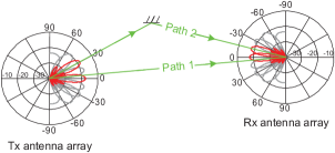
(a) The achievable data rate by using the received power of the coupling coefficients is 2.5 bit/s/Hz.

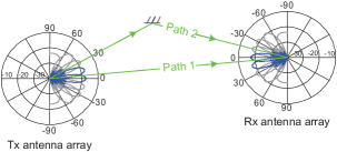
(b) The achievable data rate by using the linear combination of the two analog beamforming vectors is 3 bit/s/Hz.

Figure 2: A typical example of two different analog beam selection approaches. In the simplified two-path channel model, the AoDs are $\{5^{\circ},30^{\circ}\}$, the AoAs are $\{5^{\circ},-15^{\circ}\}$, and the difference in path attenuation between path one and two amounts to 10 dB.

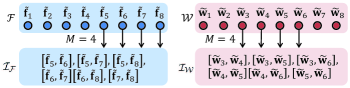
Figure 3: An example of the codebooks $\mathcal{F}$ and $\mathcal{W}$ with eight columns and the sets $\mathcal{I_{F}}$ and $\mathcal{I_{W}}$ respectively consisting of $\binom{M}{N_{RF}}=\binom{4}{2}=6$ candidates of $\mathbf{F}_{P}$ and $\mathbf{W}_{P}$.

IV Hybrid Beamforming Algorithm Based on Implicit CSI

IV-A Initial analog beam selection

To begin with, let us see how to obtain the sets $\mathcal{I_{F}}$ and $\mathcal{I_{W}}$ in (8) from the given codebooks $\mathcal{F}$ and $\mathcal{W}$. We call this step initial analog beam selection. Since the hardware-constrained analog beamforming matrices, $\mathbf{F}_{P}$ and $\mathbf{W}_{P}$, cannot be replaced by the identity matrices, we have to train all or some of the columns of the codebooks $\mathcal{F}=\{\tilde{\mathbf{f}}_{n_{f}},n_{f}=1,\cdots,N_{F}\}$ and $\mathcal{W}=\{\tilde{\mathbf{w}}_{n_{w}},n_{w}=1,\cdots,N_{W}\}$ by transmitting known pilot signals $\{s[k]\}_{k=0}^{K-1}$ satisfying $|s[k]|^{2}=1\>\forall k$.

Then, an observation used for the analog beam selection at subcarrier $k$ with respect to a trained beam pair $(\tilde{\mathbf{f}}_{n_{f}},\tilde{\mathbf{w}}_{n_{w}})$ is obtained by correlating the received signal with its transmitted pilot

$$y_{n_{w},n_{f}}[k] =\frac{s^{*}[k]}{|s[k]|^{2}}\underset{\text{received pilot}}{\underbrace{\left(\sqrt{\rho}\tilde{\mathbf{w}}_{n_{w}}^{H}\mathbf{H}[k]\tilde{\mathbf{f}}_{n_{f}}s[k]+\tilde{\mathbf{w}}_{n_{w}}^{H}\mathbf{n}[k]\right)}}$$ (9)

$$=\sqrt{\rho}\tilde{\mathbf{w}}_{n_{w}}^{H}\mathbf{H}[k]\tilde{\mathbf{f}}_{n_{f}}+z_{n_{w},n_{f}}[k],$$

where the effective noise $z_{n_{w},n_{f}}[k]\sim\mathcal{CN}(0,\sigma_{n}^{2})$ still has a Gaussian distribution with mean zero and variance $\sigma_{n}^{2}$ and similar observations become available on all subcarriers $k=0,\cdots,K-1$. The observation $y_{n_{w},n_{f}}[k]$ can also be viewed as a coupling coefficient of the channel and the beam pair $(\tilde{\mathbf{f}}_{n_{f}},\tilde{\mathbf{w}}_{n_{w}})$.

Borrowing the idea from our previous works in [11, 16], it shows that if the columns of $\mathcal{F}$ and $\mathcal{W}$ are orthogonal, the sum of the power of $K$ observations in one OFDM symbol can be directly used for the analog beam selection. As a result, $M$ (assume $M\geq N_{RF}$) analog beam pairs can be selected individually and sequentially according to the sorted received power estimates

$$\begin{gathered}(\hat{\mathbf{f}}_{P,m},\hat{\mathbf{w}}_{P,m})={\displaystyle\underset{\scriptsize\begin{array}[]{c}\tilde{\mathbf{f}}_{n_{f}}\in\mathcal{F}\backslash\mathcal{F}^{\prime},\tilde{\mathbf{w}}_{n_{w}}\in\mathcal{W}\backslash\mathcal{W}^{\prime}\end{array}}{\arg\,\max}}\sum_{k=0}^{K-1}\left|y_{n_{w},n_{f}}[k]\right|^{2},\end{gathered}$$ (10)

where $m=1,\cdots,M$, $\mathcal{F}^{\prime}=\{\hat{\mathbf{f}}_{P,n},n=1,\cdots,m-1\}$ and $\mathcal{W}^{\prime}=\{\hat{\mathbf{w}}_{P,n},n=1,\cdots,m-1\}$ are the sets consisting of the selected analog beamforming vectors from iteration $1$ to $m-1$. We assume that $M\geq N_{RF}$ for the reason that the first $N_{RF}$ selected analog beam pairs according to the sorted magnitude of $\sum_{k=0}^{K-1}|y_{n_{w},n_{f}}[k]|^{2}$ may not always lead to a good solution because we do not yet consider the effect of digital beamforming during the analog beam selection phase. To find the optimal solution, one has to further take into account the linear combination of $N_{RF}$ analog beamforming vectors selected from $\{\hat{\mathbf{f}}_{P,m}\,\forall m\}$ and $\{\hat{\mathbf{w}}_{P,m}\,\forall m\}$ with coefficients in digital beamforming.

After selecting $M$ analog beam pairs, we define two sets $\mathcal{I_{F}}$ and $\mathcal{I_{W}}$ consisting of all the combinations of any $N_{RF}$ distinct analog beamforming vectors selected from $\{\hat{\mathbf{f}}_{P,m},m=1,\cdots,M\}$ and $\{\hat{\mathbf{w}}_{P,m},m=1,\cdots,M\}$, respectively, which can be written as

$$\mathcal{I_{F}} =\{\overline{\mathbf{F}}_{P,i_{f}},i_{f}=1,\cdots,I_{F}\},$$ (11)

$$\mathcal{I_{W}} =\{\overline{\mathbf{W}}_{P,i_{w}},i_{w}=1,\cdots,I_{W}\},$$

where the cardinality $I_{F}=I_{W}=\binom{M}{N_{RF}}$ of both sets is given by the binomial coefficient. The notation $\overline{\mathbf{F}}_{P,i_{f}}$ and $\overline{\mathbf{W}}_{P,i_{w}}$ respectively denote the $i_{f}^{\text{th}}$ and $i_{w}^{\text{th}}$ candidates of the analog beamforming matrices $\mathbf{F}_{P}$ and $\mathbf{W}_{P}$. When $M$ becomes large, there is a high probability that $\mathcal{I_{F}}$ and $\mathcal{I_{W}}$ include the global optimum solution $\mathbf{F}_{P,Opt}$ and $\mathbf{W}_{P,Opt}$.

Schematic example: let us consider a scenario with $N_{T}=N_{R}=8$ antenna elements, codebook sizes $N_{F}=N_{W}=8$, orthogonal codebooks $\mathcal{F}=\mathcal{W}$ with steering angles given by $\{-90^{\circ}(\text{or }90^{\circ}),-48.59^{\circ},-30^{\circ},-14.48^{\circ},0^{\circ},14.48^{\circ},30^{\circ}$
$,48.59^{\circ}\}$, and $N_{RF}=2$ available RF chains to transmit $N_{S}=2$ data streams at $\text{SNR}=5\text{ dB}$.

The channel realization as depicted in Fig. 2 has two paths. First, in Fig. 2(a), two analog beam pairs highlighted in red are selected according to the sorted power level estimates and steer towards these two paths. Before digital beamforming comes into play, the analog beamforming vectors would be used with the same weighting. If more than $N_{RF}=2$ analog beam pairs are reserved according to the selection criterion expressed in (10), more options with digital beamforming can be explored. In this example, with $M=4$, we have $I_{F}=I_{W}=\binom{M}{N_{RF}}=\binom{4}{2}=6$ members in both $\mathcal{I_{F}}$ and $\mathcal{I_{W}}$, see Fig. 3. We can enumerate them explicitly as

$$\mathcal{I_{F}} =\{\overline{\mathbf{F}}_{P,i_{f}},i_{f}=1,\cdots,6\},$$

$$\mathcal{I_{W}} =\{\overline{\mathbf{W}}_{P,i_{w}},i_{w}=1,\cdots,6\}.$$

For instance, $\overline{\mathbf{F}}_{P,1}=[\tilde{\mathbf{f}}_{5},\tilde{\mathbf{f}}_{6}]$ and $\overline{\mathbf{W}}_{P,1}=[\tilde{\mathbf{w}}_{3},\tilde{\mathbf{w}}_{4}]$. Then, one can try all 36 pairs of the members of $\mathcal{I_{F}}$ and $\mathcal{I_{W}}$ to determine the optimal weightings in digital beamforming and choose the beam pairs yielding the maximum throughput, which will be detailed in the following subsections. In general, there will be a competition between spatial multiplexing gain over different propagation paths and power gain available from the dominant path. In this case, as shown in Fig. 2(b) with the beams highlighted in blue, the two analog beam pairs steering to the dominant path lead to higher spectral efficiency. However, which beamforming strategy has higher throughput in any specific case is not clear beforehand.

IV-B Digital beamforming

After the initial analog beam selection, we are in possession of the two sets $\mathcal{I_{F}}$ and $\mathcal{I_{W}}$ that contain the candidates of $\mathbf{F}_{P}$ and $\mathbf{W}_{P}$, and the objective is to rapidly find which pair is the optimal. Before going into the detail of our proposed scheme, let us review the relationship between the analog and digital beamforming. Given one particular choice $(\overline{\mathbf{F}}_{P,i_{f}},\overline{\mathbf{W}}_{P,i_{w}})$ selected from the candidate sets $\mathcal{I_{F}}$ and $\mathcal{I_{W}}$, it is clear that the goal of digital beamforming is to maximize the local maximum throughput $I_{LM}(\overline{\mathbf{F}}_{P,i_{f}},\overline{\mathbf{W}}_{P,i_{w}})$ as defined in (8). As a consequence, for each subcarrier the digital beamforming problem can be formulated as a throughput maximization problem subject to the power constraints, which can be stated as

$$\begin{gathered}(\overline{\mathbf{F}}_{B,i}[k],\overline{\mathbf{W}}_{B,i}[k])={\displaystyle\underset{\mathbf{F}_{B}[k],\mathbf{W}_{B}[k]}{\arg\,\max}}I(\overline{\mathbf{F}}_{P,i_{f}},\overline{\mathbf{W}}_{P,i_{w}},\mathbf{F}_{B}[k],\mathbf{W}_{B}[k])\\ \text{s.t. }\begin{cases}\text{tr}\left(\overline{\mathbf{F}}_{P,i_{f}}\mathbf{F}_{B}[k]\mathbf{R}_{s}\mathbf{F}_{B}^{H}[k]\overline{\mathbf{F}}_{P,i_{f}}^{H}\right)=\text{tr}(\mathbf{R}_{s}),\\ \mathbf{W}_{B}^{H}[k]\overline{\mathbf{W}}_{P,i_{w}}^{H}\overline{\mathbf{W}}_{P,i_{w}}\mathbf{W}_{B}[k]=\mathbf{I}_{N_{S}},\end{cases}\end{gathered}$$ (12)

where $i=(i_{f}-1)I_{W}+i_{w}$ is the index specifying the combined elements from $\mathcal{I_{F}}$ and $\mathcal{I_{W}}$.

In this problem, given ($\overline{\mathbf{F}}_{P,i_{f}},\overline{\mathbf{W}}_{P,i_{w}})$, the corresponding optimal digital beamforming matrices are given by (a detailed description of this part can be found in the journal version of this paper [17])

$$\overline{\mathbf{F}}_{B,i}[k] =\left(\overline{\mathbf{F}}_{P,i_{f}}^{H}\overline{\mathbf{F}}_{P,i_{f}}\right)^{-0.5}\left[\mathbf{V}_{E,i}[k]\right]_{:,1:N_{S}},$$ (13)

$$\overline{\mathbf{W}}_{B,i}[k] =\left(\overline{\mathbf{W}}_{P,i_{w}}^{H}\overline{\mathbf{W}}_{P,i_{w}}\right)^{-0.5}\left[\mathbf{U}_{E,i}[k]\right]_{:,1:N_{S}},$$

where the columns of $\mathbf{V}_{E,i}[k]$ and $\mathbf{U}_{E,i}[k]$ are respectively the right and left singular vectors of the effective channel

$$\mathbf{H}_{E,i}[k] \;\triangleq(\overline{\mathbf{W}}_{P,i_{w}}^{H}\overline{\mathbf{W}}_{P,i_{w}})^{-0.5}\overline{\mathbf{W}}_{P,i_{w}}^{H}\mathbf{H}[k]\overline{\mathbf{F}}_{P,i_{f}}(\overline{\mathbf{F}}_{P,i_{f}}^{H}\overline{\mathbf{F}}_{P,i_{f}})^{-0.5}$$ (14)

$$\overset{\text{SVD}}{=}\mathbf{U}_{E,i}[k]\boldsymbol{\mathbf{\Sigma}}_{E,i}[k]\mathbf{V}_{E,i}^{H}[k].$$

IV-C Key parameter of hybrid beamforming gain

Given a pair of elements selected from $\mathcal{I_{F}}$ and $\mathcal{I_{W}}$ and the corresponding optimal digital beamforming matrices across all subcarriers, we can evaluate the local maximum throughput as

$$I_{LM}(\overline{\mathbf{F}}_{P,i_{f}},\overline{\mathbf{W}}_{P,i_{w}})$$ (15)

$$=\sum_{k=0}^{K-1}\sum_{n_{s}=1}^{N_{S}}\log_{2}\left(1+\frac{\rho}{\sigma_{n}^{2}}\left[\boldsymbol{\mathbf{\Sigma}}_{E,i}^{2}[k]\right]_{n_{s},n_{s}}\left[\mathbf{R}_{s}\right]_{n_{s},n_{s}}\right),$$

where the diagonal elements of $\boldsymbol{\mathbf{\Sigma}}_{E,i}[k]$ are the singular values of the effective channel $\mathbf{H}_{E,i}[k]$. Based on the candidate set $\{(\overline{\mathbf{F}}_{P,i_{f}},\overline{\mathbf{W}}_{P,i_{w}})\,|\,\forall i_{f},i_{w}\}$, the pair leading to the maximum throughput provides the best approximation of the global optimal analog beamforming matrices, denoted as $(\hat{\mathbf{F}}_{P},\hat{\mathbf{W}}_{P})$, as well as the solution to the hybrid beamforming problem in (8),

$$\left(\hat{\mathbf{F}}_{P},\hat{\mathbf{W}}_{P}\right) ={\displaystyle\underset{\scriptsize\begin{array}[]{c}\overline{\mathbf{F}}_{P,i_{f}}\in\mathcal{I_{F}},\overline{\mathbf{W}}_{P,i_{w}}\in\mathcal{I_{W}}\end{array}}{\arg\,\max}}\,I_{LM}(\overline{\mathbf{F}}_{P,i_{f}},\overline{\mathbf{W}}_{P,i_{w}}).$$ (16)

However, this way of solving the problem requires the SVD of $\{\mathbf{H}_{E,i}[k]\}_{k=0}^{K-1}$ to obtain $I_{LM}(\overline{\mathbf{F}}_{P,i_{f}},\overline{\mathbf{W}}_{P,i_{w}})$ for each pair, which means that we have to repeat the calculation as many as $\binom{M}{N_{RF}}^{2}$ times.

To reduce the potentially large computational burden, we ask ourselves what are the crucial parameter(s) or indicator(s) that actually determine the throughput. To answer this question, let $\mathbf{R}_{s}=\frac{1}{N_{S}}\mathbf{I}_{N_{S}}$ (equal power allocation) so that the maximum achievable throughput at subcarrier $k$ becomes

$$I\left(\overline{\mathbf{F}}_{P,i_{f}},\overline{\mathbf{W}}_{P,i_{w}},\overline{\mathbf{F}}_{B,i}[k],\overline{\mathbf{W}}_{B,i}[k]\right)$$ (17)

$$\qquad\qquad=\sum_{n_{s}=1}^{N_{S}}\log_{2}\left(1+\gamma\left[\boldsymbol{\mathbf{\Sigma}}_{E,i}^{2}[k]\right]_{n_{s},n_{s}}\right),$$

where $\gamma=\frac{\rho}{N_{S}\sigma_{n}^{2}}$ is the SNR. To find the key parameter of the hybrid beamforming gain, we focus on the low SNR regime. Using the fact that $\log(1+\gamma x)\approx\gamma x$ as $\gamma\rightarrow 0$, the achievable data rate in (17) can be approximated by

$$I\left(\overline{\mathbf{F}}_{P,i_{f}},\overline{\mathbf{W}}_{P,i_{w}},\overline{\mathbf{F}}_{B,i}[k],\overline{\mathbf{W}}_{B,i}[k]\right) \overset{\gamma\rightarrow 0}{\approx}\gamma\sum_{n_{s}=1}^{N_{S}}\left[\boldsymbol{\mathbf{\Sigma}}_{E,i}^{2}[k]\right]_{n_{s},n_{s}}$$ (18)

$$\ \propto\sum_{n_{s}=1}^{N_{S}}\left[\boldsymbol{\mathbf{\Sigma}}_{E,i}^{2}[k]\right]_{n_{s},n_{s}}$$

$$\ \overset{}{\leq}\left\|\mathbf{H}_{E,i}[k]\right\|_{F}^{2}$$

with equality iff $N_{RF}=N_{S}$. For the case of $N_{RF}>N_{S}$, $\left\|\mathbf{H}_{E,i}[k]\right\|_{F}^{2}$ corresponds to the sum of all $N_{RF}$ (instead of only the $N_{S}$ strongest) eigenvalues of $\mathbf{H}_{E,i}[k]\mathbf{H}_{E,i}^{H}[k]$. Assuming that the sum of the weaker $N_{RF}-N_{S}$ eigenvalues of $\mathbf{H}_{E,i}[k]\mathbf{H}_{E,i}^{H}[k]$ is small, the approximation of $\sum_{n_{s}=1}^{N_{S}}\left[\boldsymbol{\mathbf{\Sigma}}_{E,i}^{2}[k]\right]_{n_{s},n_{s}}$ by $\left\|\mathbf{H}_{E,i}[k]\right\|_{F}^{2}$ seems to be valid for most cases of interest.

Fortunately, the matrix $\mathbf{H}_{E,i}[k]$ can be easily obtained from the original observations $\{y_{n_{w},n_{f}}[k]\,\forall n_{w},n_{f},k\}$ [16]. Let us show the effective channel in (14) again and approximate the matrix $\overline{\mathbf{W}}_{P,i_{w}}^{H}\mathbf{H}[k]\overline{\mathbf{F}}_{P,i_{f}}$ by $\mathbf{Y}_{i}[k]$ (the elements of $\mathbf{Y}_{i}[k]$ can be collected from the observations),

$$\mathbf{H}_{E,i}[k] \triangleq(\overline{\mathbf{W}}_{P,i_{w}}^{H}\overline{\mathbf{W}}_{P,i_{w}})^{-0.5}\underset{\approx\mathbf{Y}_{i}[k]}{\underbrace{\overline{\mathbf{W}}_{P,i_{w}}^{H}\mathbf{H}[k]\overline{\mathbf{F}}_{P,i_{f}}}}(\overline{\mathbf{F}}_{P,i_{f}}^{H}\overline{\mathbf{F}}_{P,i_{f}})^{-0.5}$$ (19)

$$\approx(\overline{\mathbf{W}}_{P,i_{w}}^{H}\overline{\mathbf{W}}_{P,i_{w}})^{-0.5}\mathbf{Y}_{i}[k](\overline{\mathbf{F}}_{P,i_{f}}^{H}\overline{\mathbf{F}}_{P,i_{f}})^{-0.5}$$

$$\triangleq\hat{\mathbf{H}}_{E,i}[k].$$

For example, if $\overline{\mathbf{F}}_{P,i_{f}}=[\tilde{\mathbf{f}}_{P,1},\cdots,\tilde{\mathbf{f}}_{P,N_{RF}}]$ and $\overline{\mathbf{W}}_{P,i_{w}}=[\tilde{\mathbf{w}}_{P,1},\cdots,\tilde{\mathbf{w}}_{P,N_{RF}}]$, where $\tilde{\mathbf{f}}_{P,n_{rf}}$ is the $n_{rf}^{\text{th}}$ column of $\mathcal{F}$ and $\tilde{\mathbf{w}}_{P,n_{rf}}$ is the $n_{rf}^{\text{th}}$ column of $\mathcal{W}$, one has

$$\mathbf{Y}_{i}[k] =\left[\begin{array}[]{ccc}y_{1,1}[k]&\cdots&y_{1,N_{RF}}[k]\\ \vdots&\ddots&\vdots\\ y_{N_{RF},1}[k]&\cdots&y_{N_{RF},N_{RF}}[k]\end{array}\right]$$ (20)

$$=\overline{\mathbf{W}}_{P,i_{w}}^{H}\mathbf{H}[k]\overline{\mathbf{F}}_{P,i_{f}}+\mathbf{Z}[k].$$

Therefore, given a pair $(\overline{\mathbf{F}}_{P,i_{f}},\overline{\mathbf{W}}_{P,i_{w}})$ selected from $\mathcal{I_{F}}$ and $\mathcal{I_{W}}$, we can rapidly obtain the approximation of $\mathbf{H}_{E,i}[k]$, denoted as $\hat{\mathbf{H}}_{E,i}[k]$ in (19).

To conclude, the proposed solution can be stated as: first obtain the candidate sets ($\mathcal{I_{F}}$ and $\mathcal{I_{W}}$) and the approximation of $\mathbf{H}_{E,i}[k]$ ($\hat{\mathbf{H}}_{E,i}[k]$) from the observations $\{y_{n_{w},n_{f}}[k]\,\forall n_{w},n_{f},k\}$ and then solve the maximization problem in (16), which can be rewritten as

$$\left(\hat{i}_{f},\hat{i}_{w}\right) ={\displaystyle\underset{\scriptsize\begin{array}[]{c}\overline{\mathbf{F}}_{P,i_{f}}\in\mathcal{I_{F}},\overline{\mathbf{W}}_{P,i_{w}}\in\mathcal{I_{W}}\end{array}}{\arg\,\max}}\,I_{LM}(\overline{\mathbf{F}}_{P,i_{f}},\overline{\mathbf{W}}_{P,i_{w}})$$ (21)

$$\approx{\displaystyle\underset{\scriptsize\begin{array}[]{c}\overline{\mathbf{F}}_{P,i_{f}}\in\mathcal{I_{F}},\overline{\mathbf{W}}_{P,i_{w}}\in\mathcal{I_{W}}\\ i=(i_{f}-1)I_{W}+i_{w}\end{array}}{\arg\,\max}}\sum_{k=0}^{K-1}\left\|\hat{\mathbf{H}}_{E,i}[k]\right\|_{F}^{2}.$$

According to the index pair $(\hat{i}_{f},\hat{i}_{w})$, we have the selected analog and corresponding digital beamforming matrices given by

$$\hat{\mathbf{F}}_{P} =\overline{\mathbf{F}}_{P,\hat{i}_{f}},$$ (22)

$$\hat{\mathbf{W}}_{P} =\overline{\mathbf{W}}_{P,\hat{i}_{w}},$$

$$\hat{\mathbf{F}}_{B}[k] =(\hat{\mathbf{F}}_{P}^{H}\hat{\mathbf{F}}_{P})^{-0.5}\left[\hat{\mathbf{V}}_{E,\hat{i}}[k]\right]_{:,1:N_{S}},$$

$$\hat{\mathbf{W}}_{B}[k] =(\hat{\mathbf{W}}_{P}^{H}\hat{\mathbf{W}}_{P})^{-0.5}\left[\hat{\mathbf{U}}_{E,\hat{i}}[k]\right]_{:,1:N_{S}},$$

where $\hat{i}=(\hat{i}_{f}-1)I_{W}+\hat{i}_{w}$ and $\hat{\mathbf{U}}_{E,\hat{i}}[k]\hat{\boldsymbol{\mathbf{\Sigma}}}_{E,\hat{i}}[k]\hat{\mathbf{V}}_{E,\hat{i}}^{H}[k]=\text{SVD}(\hat{\mathbf{H}}_{E,\hat{i}}[k])$. The complete proposed algorithm of the hybrid beamforming implementation based on implicit CSI (i.e., the coupling coefficients $\{y_{n_{w},n_{f}}[k]\,\forall n_{w},n_{f},k\}$) is shown in Algorithm 1, where $f(\hat{\mathbf{H}}_{E,i}[k])$ in Step 4 denotes the analog beam selection criterion by using (17) or (18) with the argument $\hat{\mathbf{H}}_{E,i}[k]$ as

$$f\left(\hat{\mathbf{H}}_{E,i}[k]\right)$$

$$=\begin{cases}\sum_{n_{s}=1}^{N_{S}}\log_{2}\left(1+\gamma\left[\hat{\boldsymbol{\mathbf{\Sigma}}}_{E,i}^{2}[k]\right]_{n_{s},n_{s}}\right),&\text{w/o approx.}\\ \left\|\hat{\mathbf{H}}_{E,i}[k]\right\|_{F}^{2},&\text{w/ approx.}\end{cases}$$ (23)

The advantages of the proposed algorithm are summarized as follows: (1) we can omit high-dimensional channel estimation problems, and (2) even though the cardinalities of $\mathcal{I_{F}}$ and $\mathcal{I_{W}}$ are large, the computational overhead is minor because we just need to calculate the Frobenius norm of the effective channel matrices, whose elements can be easily obtained from the observations $\{y_{n_{w},n_{f}}[k]\,\forall n_{w},n_{f},k\}$.

In (17), we simply assume that the transmit power is equally allocated to $N_{S}$ data streams to facilitate the process of finding the best value of the key parameter. Once the analog and digital beamforming matrices are selected, the global maximum throughput can be further improved by optimizing the power allocation (i.e., by a water-filling power allocation scheme [15]) for $N_{S}$ data streams according to the effective channel condition $\hat{\mathbf{H}}_{E,\hat{i}}[k]$ at each subcarrier.

Algorithm 1: Hybrid beamforming based on implicit CSI
Input: $\{y_{n_{w},n_{f}}[k]\,\forall n_{w},n_{f},k\}$
Output: $\hat{\mathbf{F}}_{P}$, $\hat{\mathbf{W}}_{P}$, $(\hat{\mathbf{F}}_{B}[k],\hat{\mathbf{W}}_{B}[k])\,\forall k$
1.	Given $\{y_{n_{w},n_{f}}[k]\,\forall n_{w},n_{f},k\}$, select $M$ analog beam pairs
	$(\hat{\mathbf{f}}_{P,m},\hat{\mathbf{w}}_{P,m})$, where $m=1,\cdots,M$, according to (10).
2.	Generate two candidate sets $\mathcal{I_{F}}$ and $\mathcal{I_{W}}$ based on $\{\hat{\mathbf{f}}_{P,m}\,\forall m\}$
	and $\{\hat{\mathbf{w}}_{P,m}\,\forall m\}$, respectively.
3.	$\hat{\mathbf{H}}_{E,i}[k]=(\overline{\mathbf{W}}_{P,i_{w}}^{H}\overline{\mathbf{W}}_{P,i_{w}})^{-0.5}\mathbf{Y}_{i}[k](\overline{\mathbf{F}}_{P,i_{f}}^{H}\overline{\mathbf{F}}_{P,i_{f}})^{-0.5}$,
	where $\overline{\mathbf{F}}_{P,i_{f}}\in\mathcal{I_{F}}$, $\overline{\mathbf{W}}_{P,i_{w}}\in\mathcal{I_{W}}$, and the entries of $\mathbf{Y}_{i}[k]$
	are collected from $\{y_{n_{w},n_{f}}[k]\,\forall n_{w},n_{f}\}.$
4.	$(\hat{i}_{f},\hat{i}_{w})={\displaystyle\underset{\scriptsize\begin{array}[]{c}i=(i_{f}-1)I_{W}+i_{w}\end{array}}{\arg\,\max}\sum_{k=0}^{K-1}f(\hat{\mathbf{H}}_{E,i}[k]),}$
	where $f(\hat{\mathbf{H}}_{E,i}[k])$ is given in (23).
5.	Output: $\hat{\mathbf{F}}_{P}=\overline{\mathbf{F}}_{P,\hat{i}_{f}}$ and $\hat{\mathbf{W}}_{P}=\overline{\mathbf{W}}_{P,\hat{i}_{w}}$.
6.	$\hat{\mathbf{U}}_{E,\hat{i}}[k]\hat{\boldsymbol{\mathbf{\Sigma}}}_{E,\hat{i}}[k]\hat{\mathbf{V}}_{E,\hat{i}}^{H}[k]=\text{SVD}(\hat{\mathbf{H}}_{E,\hat{i}}[k])$,
	where $\hat{i}=(\hat{i}_{f}-1)I_{W}+\hat{i}_{w}$.
7.	Output: $\begin{cases}\hat{\mathbf{F}}_{B}[k]=(\hat{\mathbf{F}}_{P}^{H}\hat{\mathbf{F}}_{P})^{-0.5}\left[\hat{\mathbf{V}}_{E,\hat{i}}[k]\right]_{:,1:N_{S}}\\ \hat{\mathbf{W}}_{B}[k]=(\hat{\mathbf{W}}_{P}^{H}\hat{\mathbf{W}}_{P})^{-0.5}\left[\hat{\mathbf{U}}_{E,\hat{i}}[k]\right]_{:,1:N_{S}}\end{cases}$

V Simulation Results

The system has $N_{T}=N_{R}=32$ antennas, $N_{RF}=2$ RF chains, $N_{S}=2$ data streams, and $K=512$ subcarriers. The cluster-based channel model has $C=5$ clusters including one line-of-sight (LoS) and four NLoS clusters, and each cluster has $R=8$ rays. The codebooks $\mathcal{F}$ and $\mathcal{W}$ have the same number of members, $N_{F}=N_{W}=32$, and $32$ steering angle candidates are: $\left\{\frac{180^{\circ}}{\pi}\cdot\sin^{-1}\left(\frac{\left(n_{f}-16\right)}{16}\right),\,n_{f}=1,\cdots,32\right\}$, which yield orthogonal codebooks [18].

We chose the work in [5] that implements hybrid beamforming based on the singular vectors of $\mathbf{H}[k]\>\forall k$ (i.e., explicit CSI) as a reference method for comparison and extended it from single carrier to multiple carriers. Different to the reference scheme, Algorithm 1 uses the received coupling coefficients (i.e., implicit CSI) as the observations for the hybrid beamforming implementation. The received coupling coefficients are commonly used for channel estimation [9, 19], but in this paper we use them to directly implement the hybrid beamforming on both sides. As a result, we can get rid of the overhead of channel estimation.

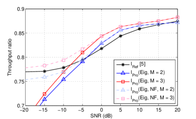
Figure 4: Normalized achievable throughput by the proposed and reference methods. In the proposed method, different number $M$ of initially selected analog beam pairs as well as different qualities of observations are evaluated.

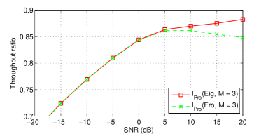
Figure 5: Curve $I_{Pro}(Eig,M=3)$ shown in Fig. 4 and its approximation achieved by using the key parameter.

To clearly present the difference in throughput by using different methods, the calculated throughput values are normalized to the throughput achieved by fully digital beamforming. Fig. 4 shows the achievable data rates with $M=2,3$ initially selected analog beam pairs in the proposed method (curves denoted as $I_{Pro}$) and the reference approach (curve $I_{Ref}$). The data rates shown in $I_{Pro}(Eig,M=2,3)$ are calculated by

$$\frac{1}{K}\sum_{k=0}^{K-1}I(\hat{\mathbf{F}}_{P},\hat{\mathbf{W}}_{P},\hat{\mathbf{F}}_{B}[k],\hat{\mathbf{W}}_{B}[k]),$$ (24)

where $(\hat{\mathbf{F}}_{P},\hat{\mathbf{W}}_{P},\hat{\mathbf{F}}_{B}[k],\hat{\mathbf{W}}_{B}[k])$ are the outputs of Algorithm 1 with $f(\hat{\mathbf{H}}_{E,i}[k])=\sum_{n_{s}=1}^{N_{S}}\log_{2}(1+\gamma[\hat{\boldsymbol{\mathbf{\Sigma}}}_{E,i}^{2}[k]]_{n_{s},n_{s}})$ in Step 4. If the inputs of Algorithm 1, $\{y_{n_{w},n_{f}}[k]\,\forall n_{w},n_{f},k\}$, do not take into account random noise signals, repeating the above-mentioned steps leads to $I_{Pro}(Eig,N\!F,M\!=\!2,3)$. $I_{Ref}$ is also calculated by (24) with the solution of $(\mathbf{F}_{P},\mathbf{W}_{P},\mathbf{F}_{B}[k],\mathbf{W}_{B}[k])$ given in [5]. Furthermore, in Fig. 5, curve $I_{Pro}(Fro,M=3)$ uses the Frobenius norm of $\hat{\mathbf{H}}_{E,i}[k]$ (i.e., the key parameter of the hybrid beamforming gain) as a selection criterion in Algorithm 1 Step 4 to find $(\hat{\mathbf{F}}_{P},\hat{\mathbf{W}}_{P},\hat{\mathbf{F}}_{B}[k],\hat{\mathbf{W}}_{B}[k])$.

In Fig. 4, we can find that when $\text{SNR}>0\text{ dB}$, the observations with and without noise effect in the proposed method yield almost the same throughput. Then, to better compare our approach with $I_{Ref}$, let us see curves $I_{Pro}(Eig,N\!F,M=3)$ and $I_{Ref}$. It is obvious that $I_{Pro}(Eig,N\!F,M=3)$ achieves higher data rates than $I_{Ref}$. Although these two methods use different ways to construct the hybrid beamforming, we try an explanation based on some assumptions. Assume that these two schemes find the same $N_{RF}$ analog beam pairs, which means that they have the same effective channel. In this case, Algorithm 1 uses the SVD of the effective channel to find the solution of digital beamforming matrices. From [15], we know that this solution is the optimal. In contrast, the digital beamforming in [5] uses the least-squares solution, which is sub-optimal. When we reserve more candidates ($M>N_{RF}$), there is a higher probability that both algorithms find the same $N_{RF}$ analog beam pairs. If so, Algorithm 1 theoretically outperforms the reference method.

Next, in Fig. 5, when $\text{SNR}<5\text{ dB}$, $I_{Pro}(Fro,M=3)$ achieves almost the same data rates as $I_{Pro}(Eig,M=3)$, which means that the approximation error between $\sum_{n_{s}=1}^{N_{S}}\log_{2}(1+\gamma[\hat{\boldsymbol{\mathbf{\Sigma}}}_{E,i}^{2}[k]]_{n_{s},n_{s}})$ and $||\hat{\mathbf{H}}_{E,i}[k]||_{F}^{2}$ (see (23)) is small in the low SNR regime. From Fig. 4 and Fig. 5, we can see that if the system operates in the SNR range between $-5$ and $5$ dB, the Frobenius norm of the estimated effective channel works pretty well.

VI Conclusion

This paper presents a novel strategy to implement the hybrid beamforming matrices at the transmitter and receive based on the received coupling coefficients. As a result, the high-dimensional channel estimation and singular value decomposition are unnecessary. The idea behind this approach is simple: efficiently evaluating the key parameter, such as the Frobenius norm of the effective channel matrices, to implement the hybrid beamforming based on the estimates of received power levels. Since the key parameter of the hybrid beamforming gain is a function of the effective channel matrix, which has much lower dimension typically, it is not difficult to try a (small) set of possible alternatives to find a reasonable approximation of the optimal hybrid beamforming. Moreover, the effective channel matrix can be obtained from the received coupling coefficients. This avoids acquiring the explicit channel estimation and knowledge of the specific angles of the propagation paths. Instead, the implicit channel knowledge that which beam pairs produce the strongest coupling between transmitter and receiver is enough in a sense.

References

- [1] T. Rappaport, R. Heath, R. Daniels, and J. Murdock, Millimeter Wave Wireless Communications. Prentice Hall, 2014.
- [2] A. Hajimiri, H. Hashemi, A. Natarajan, X. Guan, and A. Komijani, “Integrated phased array systems in silicon,” Proc. IEEE, vol. 93, no. 9, pp. 1637–1655, Sep. 2005.
- [3] J. Liberti and T. Rappaport, Smart antennas for wireless communications: IS-95 and third generation CDMA applications. Prentice Hall, 1999.
- [4] H. L. Van Trees, Optimum Array Processing: Part IV of Detection, Estimation, and Modulation Theory. Wiley, 2002.
- [5] O. E. Ayach, R. W. Heath, S. Abu-Surra, S. Rajagopal, and Z. Pi, “Low complexity precoding for large millimeter wave MIMO systems,” in IEEE Int. Conf. on Commun. (ICC), Ottawa, ON, Canada, Jun. 2012, pp. 3724–3729.
- [6] A. Alkhateeb and R. W. Heath, “Frequency selective hybrid precoding for limited feedback millimeter wave systems,” IEEE Trans. Commun., vol. 64, no. 5, pp. 1801–1818, May 2016.
- [7] F. Sohrabi and W. Yu, “Hybrid digital and analog beamforming design for large-scale antenna arrays,” IEEE J. Sel. Topics Signal Process., vol. 10, no. 3, pp. 501–513, Apr. 2016.
- [8] H. L. Chiang, T. Kadur, W. Rave, and G. Fettweis, “Low-complexity spatial channel estimation and hybrid beamforming for millimeter wave links,” in IEEE Int. Symp. on Personal, Indoor and Mobile Radio Commun. (PIMRC), Valencia, Spain, Sep. 2016, pp. 942–948.
- [9] H. L. Chiang, W. Rave, T. Kadur, and G. Fettweis, “Full rank spatial channel estimation at millimeter wave systems,” in Int. Symp. on Wireless Commun. Syst. (ISWCS), Poznan, Poland, Sep. 2016, pp. 42–48.
- [10] K. Venugopal, A. Alkhateeb, R. W. Heath, and N. G. Prelcic, “Time-domain channel estimation for wideband millimeter wave systems with hybrid architecture,” in IEEE Int. Conf. on Acoust., Speech and Signal Process. (ICASSP), New Orleans, LA, USA, Mar. 2017, pp. 6493–6497.
- [11] H. L. Chiang, W. Rave, T. Kadur, and G. Fettweis, “A low-complexity beamforming method by orthogonal codebooks for millimeter wave links,” in IEEE Int. Conf. on Acoust., Speech and Signal Process. (ICASSP), New Orleans, LA, USA, Mar. 2017, pp. 3375 – 3379.
- [12] T. T. Cai and L. Wang, “Orthogonal matching pursuit for sparse signal recovery with noise,” IEEE Trans. Inf. Theory, vol. 57, no. 7, pp. 4680–4688, Jul. 2011.
- [13] T. S. Rappaport, G. R. MacCartney, M. K. Samimi, and S. Sun, “Wideband millimeter-wave propagation measurements and channel models for future wireless communication system design,” IEEE Trans. Commun., vol. 63, no. 9, pp. 3029–3056, Sep. 2015.
- [14] 3GPP TR 38.900 V14.3.1, “Study on channel model for frequency spectrum above 6 GHz (Release 14),” Tech. Rep., 2017.
- [15] E. Telatar, “Capacity of multi-antenna gaussian channels,” European Trans. on Telecommun., vol. 10, pp. 585–595, 1999.
- [16] H. L. Chiang, W. Rave, T. Kadur, and G. Fettweis, “Hybrid beamforming strategy for wideband millimeter wave channel models,” in Int. ITG Workshop on Smart Antennas (WSA), Berlin, Germany, Sep. 2017, pp. 1 – 7.
- [17] ——, “Hybrid beamforming based on implicit channel state information for millimeter wave links,” Sep. 2017. [Online]. Available: https://arxiv.org/abs/1709.07273
- [18] H. L. Chiang, T. Kadur, and G. Fettweis, “Analyses of orthogonal and non-orthogonal steering vectors at millimeter wave systems,” in IEEE Int. Symp. on A World of Wireless, Mobile and Multimedia Networks (WoWMoM), Coimbra, Portugal, Jun. 2016, pp. 1–6.
- [19] R. Méndez-Rial, C. Rusu, N. González-Prelcic, A. Alkhateeb, and R. W. Heath, “Hybrid MIMO architectures for millimeter wave communications: Phase shifters or switches?” IEEE Access, vol. 4, pp. 247–267, 2016.