Sequentializing cellular automata

Abstract

We study the problem of sequentializing a cellular automaton without introducing any intermediate states, and only performing reversible permutations on the tape. We give a decidable characterization of cellular automata which can be written as a single left-to-right sweep of a bijective rule from left to right over an infinite tape.

1 Introduction

Cellular automata (CA) are models of parallel computation, so when implementing them on a sequential architecture, one cannot simply update the cells one by one – some cells would see already updated states and the resulting configuration would be incorrect. The simplest-to-implement solution is to hold two copies of the current configuration in memory, and map $(x,x)\mapsto(x,G(x))\mapsto(G(x),G(x))$. This is wasteful in terms of memory, and one can, with a bit of thinking, reduce the memory usage to a constant by simply remembering a ‘wave’ containing the previous values of the $r$ cells to the left of the current cell, where $r$ is the radius of the CA.

Here, we study the situation where the additional memory usage can be, in a sense, dropped to zero – more precisely we remember only the current configuration $x\in S^{\mathbb{Z}}$, and to apply the cellular automaton we sweep a permutation $\chi:S^{m}\to S^{m}$ from left to right over $x$ (applying it consecutively to all length-$m$ subwords of $x$). The positions where the sweep starts may get incorrect values, but after a bounded number of steps, the rule should start writing the image of the cellular automaton. We formalize this in two ways, with ‘sliders’ and ‘sweepers’, which are two ways of formally dealing with the problem that sweeps ‘start from infinity’.

It turns out that the cellular automata that admit a sliding rule are precisely the ones that are left-closing (Definition 11), and whose number of right stairs (see Definition 14) of length $3m$ divides $|S|^{3m}$ for large enough $m$. This can be interpreted as saying that the average movement ‘with respect to any prime number’ is not to the right. See Theorem 20 and Theorem 28 for the precise statements, and Section 4 for decidability results.

We introduce the sweeping hierarchy where left-to-right sweeps and right-to-left sweeps alternate, and the closing hierarchy where left-closing and right-closing CA alternate. We show that the two hierarchies coincide starting from the second step. We do not know if the hierarchies collapse on a finite level.

1.1 Preliminaries

We denote the set of integers by $\mathbb{Z}$. For integers $i\leq j$ we write $[i,j)$ for $\{x\in\mathbb{Z}\mid i\leq x<j\}$ and $[i,j]$ for $[i,j)\cup\{j\}$; furthermore $[i,\infty)=\{x\in\mathbb{Z}\mid i\leq x\}$ and $(-\infty,i)=\{x\in\mathbb{Z}\mid x<i\}$ have the obvious meaning. Thus $[0,\infty)$ is the set of non-negative integers which is also denoted by $\mathbb{N}_{0}$.

Occasionally we use notation for a set $M$ of integers in a place where a list of integers is required. If no order is specified we assume the natural increasing order. If the reversed order is required we will write $M^{R}$.

For sets $A$ and $B$ the set of all functions $f:A\to B$ is denoted $B^{A}$. For $f\in B^{A}$ and $M\subseteq A$ the restriction of $f$ to $M$ is written as $f|_{M}$ or sometimes even $f_{M}$. Finite words $w\in S^{n}$ are lists of symbols, e.g. mappings $w:[0,n)\to S$. Number $n$ is the length of the word. The set of all finite words is denoted by $S^{*}$.

Configurations of one-dimensional CA are biinfinite words $x:\mathbb{Z}\to S$. Instead of $x(i)$ we often write $x_{i}$. We define the left shift $\sigma:S^{\mathbb{Z}}\to S^{\mathbb{Z}}$ by $\sigma(x)_{i}=x_{i+1}$. The restriction of $x$ to a subset $(-\infty,i)$ gives a left-infinite word for which we write $x_{(-\infty,i)}$; for a right-infinite word we write $x_{[i,\infty)}$. These are called half-infinite words. Half-infinite words can also be shifted by $\sigma$, and this is defined using the same formula. The domain is shifted accordingly so for $x\in S^{[i,\infty)}$ we have $\sigma(x)\in S^{[i-1,\infty)}$.

We use a special convention for concatenating words: Finite words ‘float’, in the sense that they live in $S^{n}$ for some $n$, without a fixed position, and $u\cdot v$ denotes the concatenation of $u$ and $v$ as an element of $S^{|u|+|v|}$. Half-infinite configurations have a fixed domain $(-\infty,i]$ or $[i,\infty)$ for some $i$, which does not change when they are concatenated with finite words or other half-infinite configurations, while finite words are shifted suitably so that they fill the gaps exactly (and whenever we concatenate, we make sure this makes sense).

More precisely, for $w\in S^{*}$ and $y\in S^{(-\infty,i]}$, we have $y\cdot w\in S^{(-\infty,i+|w|]}$ and for $w\in S^{*}$ and $z\in S^{[i,\infty)}$ we have $w\cdot z\in S^{[i-|w|,\infty)}$ (defined in the obvious way). For a word $w\in S^{*}$ and half-infinite words $y\in S^{(-\infty,i)}$ and $z\in S^{[i+n,\infty)}$ we write $y\cdot w\cdot z$ for the obvious configuration in $S^{\mathbb{Z}}$, and this is defined if and only if $|w|=n$.

The set $S^{\mathbb{Z}}$ of configurations is assigned the usual product topology generated by cylinders. A cylinder defined by word $w\in S^{n}$ at position $i\in\mathbb{Z}$ is the set

$$[w]_{[i,i+n)}=\{x\in S^{\mathbb{Z}}\ |\ x_{[i,i+n)}=w\}$$

of configurations that contain word $w$ in position $[i,i+n)$. Cylinders are open and closed, and the open sets in $S^{\mathbb{Z}}$ are precisely the unions of cylinders. We extend the notation also to half-infinite configurations, and define

$$[y]_{D}=\{x\in S^{\mathbb{Z}}\ |\ x_{D}=y\}$$

for $D=[i,\infty)$ and $D=(\infty,i]$, and any $y\in S^{D}$. These sets are closed in the topology.

2 Sliders and sweepers

A block rule is a function $\chi:S^{m}\to S^{m}$. Given a block rule $\chi$ we want to define what it means to “apply $\chi$ from left to right once at every position”. We provide two alternatives, compare them and characterize which cellular automata can be obtained by them. The first alternative, called a slider, assumes a bijective block rule $\chi$ that one can slide along a configuration left-to-right or right-to-left to transition between a configuration $y$ and its image $f(y)$. The second alternative, called a sweeper, must consistently provide values of the image $f(y)$ when sweeping left-to-right across $y$ starting sufficiently far on the left.

We first define what it means to apply a block rule on a configuration.

Definition 1.

Let $\chi:S^{m}\to S^{m}$ be a block rule and $i\in\mathbb{Z}$. The application of $\chi$ at coordinate $i$ is the function $\chi^{i}:S^{\mathbb{Z}}\longrightarrow S^{\mathbb{Z}}$ given by $\chi^{i}(x)_{[i,i+m)}=\chi(x_{[i,i+m)})$ and $\chi^{i}(x)_{j}=x_{j}$ for all $j\not\in[i,i+n)$. More generally, for $i_{1},\ldots,i_{k}\in\mathbb{Z}$ we write

$$\chi^{i_{1},\ldots,i_{k}}=\chi^{i_{k}}\circ\cdots\circ\chi^{i_{2}}\circ\chi^{i_{1}}.$$

When $m>1$, it is meaningless to speak about “applying $\chi$ to each cell simultaneously”: An application of $\chi$ changes the states of several cells at once. Applying it slightly shifted could change a certain cell again, but in a different way.

We next define finite and infinite sweeps of block rule applications with a fixed start position.

Definition 2.

Given a block rule $\chi$ for $i,j\in\mathbb{Z}$, $i\leq j$, define $\chi^{[i,j]}=\chi^{j}\circ\cdots\circ\chi^{i}$; analogously let $\chi^{[i,j)}=\chi^{j-1}\circ\cdots\circ\chi^{i}$. For any configuration $x\in S^{\mathbb{Z}}$ and fixed $i\in\mathbb{Z}$ the sequence of configurations $x^{(j)}=\chi^{[i,j]}(x)$ for $j\in[i,\infty)$ has a limit (point in the topological space $S^{\mathbb{Z}}$) for which we write ${\chi}^{i+}(x)$.

Analogously, for a block rule $\xi$ the sequence of configurations $x^{(j)}=\xi^{[j,i)^{R}}(x)$ for $j\in(-\infty,i)$ has a limit for which we write ${\xi}^{i-}(x)$.

It should be observed that in the definition of ${\chi}^{i+}(x)$ one has $i<j$ and the block rule is applied at successive positions from left to right. On the other hand $j<i$ is assumed in the definition of ${\xi}^{i-}(x)$ and since the ${}^{{}^{R}}$ in $\xi^{[j,i)^{R}}$ indicates application of $\xi$ at the positions in the reverse order, i.e. $i-1,i-2,\dots,j$, the block rule is applied from right to left.

The reason the limits always exist in the definition is that the value of $x^{(j)}_{i}$ changes at most $m$ times, on the steps where the sweep passes over the cell $i$.

Example 3.

Let $S=\{0,1\}$ and consider the block rule $\chi:S^{[0,2)}\to S^{[0,2)}:(a,b)\mapsto(b,a)$. For consistency with the above definition denote by $\xi$ the inverse of $\chi$ (which in this case happens to be $\chi$ again). Let $s\in S$ and $y\in S^{\mathbb{Z}}$. We will look at the configuration $x\in S^{\mathbb{Z}}$ with

$$x_{i}=\begin{cases}y_{i+1},&\text{ if }i<0\\ s,&\text{ if }i=0\\ y_{i},&\text{ if }i>0\end{cases}$$

The application of $\chi$ successively at positions $0,1,2,\dots$ always swaps state $s$ with its right neighbor. Since cell $j$ can only possibly change when $\chi^{j-1}$ or $\chi^{j}$ is applied, each cell enters a fixed state after a finite number of steps; see also the lower part of Figure 1 starting at the row with configuration $x$.

$\xi^{0-}(x)$  $\cdots$	$y$ _-3	$y$ _-2	$y$ _-1	$y$ _0	$y$ _1	$y$ _2	$y$ _3	$\cdots$	$y$
	$\vdots$							$\cdots$
$\xi^{[-3,0)^{R}}(x)$  $\cdots$	$s$	$y$ _-2	$y$ _-1	$y$ _0	$y$ _1	$y$ _2	$y$ _3	$\cdots$
$\xi^{[-2,0)^{R}}(x)$  $\cdots$	$y$ _-2	$s$	$y$ _-1	$y$ _0	$y$ _1	$y$ _2	$y$ _3	$\cdots$
$\xi^{[-1,0)^{R}}(x)$  $\cdots$	$y$ _-2	$y$ _-1	$s$	$y$ _0	$y$ _1	$y$ _2	$y$ _3	$\cdots$
$x\hphantom{)}$  $\cdots$	$y$ _-2	$y$ _-1	$y$ _0	$s$	$y$ _1	$y$ _2	$y$ _3	$\cdots$	$x$
$\chi^{[0,1)}(x)$  $\cdots$	$y$ _-2	$y$ _-1	$y$ _0	$y$ _1	$s$	$y$ _2	$y$ _3	$\cdots$
$\chi^{[0,2)}(x)$  $\cdots$	$y$ _-2	$y$ _-1	$y$ _0	$y$ _1	$y$ _2	$s$	$y$ _3	$\cdots$
$\chi^{[0,3)}(x)$  $\cdots$	$y$ _-2	$y$ _-1	$y$ _0	$y$ _1	$y$ _2	$y$ _3	$s$	$\cdots$
	$\vdots$							$\cdots$
$\chi^{0+}(x)$  $\cdots$	$y$ _-2	$y$ _-1	$y$ _0	$y$ _1	$y$ _2	$y$ _3	$y$ _4	$\cdots$	$z$

Figure 1: A sequence of configurations with the center cell at position $0$. Starting with configuration $x$ in the middle when going downward the swapping rule $\chi$ is applied to blocks $[0,1]$, $[1,2]$, etc., and going from $x$ upward rule $\xi=\chi$ is applied to blocks $[-1,0]$, $[-2,-1]$ and so on.

Example 4.

Let $S=\{0,1\}$ and consider the block rule $\chi:S^{[0,2)}\to S^{[0,2)}:(a,b)\mapsto(a+b,b)$. Then sliding this rule over a configuration $x\in\{0,1\}^{\mathbb{Z}}$ produces the image of $x$ in the familiar exclusive-or cellular automaton with neighborhood $\{0,1\}$ (elementary CA 102). We will see in Example 22 that the exclusive-or CA with neighborhood $\{-1,0\}$ can not be defined this way.

2.1 Definition of sliders

Definition 5.

A bijective block rule $\chi$ with inverse $\xi$ defines a slider relation $F\subset S^{\mathbb{Z}}\times S^{\mathbb{Z}}$ by $(y,z)\in F$ iff for some $x\in S^{\mathbb{Z}}$ and some $i\in\mathbb{Z}$ we have $\xi^{i-}(x)=y$ and $\chi^{i+}(x)=z$. We call the pair $(x,i)$ a representation of $(y,z)\in F$.

Note that every $(x,i)\in S^{\mathbb{Z}}\times\mathbb{Z}$ is a representation of exactly one pair, namely $(\xi^{i-}(x),\chi^{i+}(x))\in F$.

Lemma 6.

Let $(x,i)$ be a representation of $(y,z)\in F$ under a bijective block rule $\chi$ of block length $n$. Then $x_{(-\infty,i)}=z_{(-\infty,i)}$ and $x_{[i+n,\infty)}=y_{[i+n,\infty)}$.

Proof.

Applying block rule $\chi$ at positions $j\geq i$ in $x$ never changes cells at positions $k<i$. Therefore $x_{k}=({\chi}^{i+}(x))_{k}=z_{k}$ proving the first part. The second part follows analogously. ∎

Lemma 7.

Let $(y,z)\in F$ be fixed. For all $i\in\mathbb{Z}$ denote

$$R_{i}=\{x\in S^{\mathbb{Z}}\ |\ (x,i)\mbox{ is a representation of }(y,z)\}.$$

For $i<j$ the function $\chi^{[i,j)}:R_{i}\longrightarrow R_{j}$ is a bijection, with inverse $\xi^{[i,j)^{R}}$. All $R_{i}$ have the same finite cardinality.

Proof.

The claim follows directly from the definition and the facts that

$$\chi^{j+}\circ\chi^{[i,j)}=\chi^{i+}\mbox{ and }\xi^{j-}\circ\chi^{[i,j)}=\xi^{i-},$$ (1)

and that $\chi^{[i,j)}$ and $\xi^{[i,j)^{R}}$ are inverses of each other.

More precisely, if $x\in R_{i}$ then $z=\chi^{i+}(x)=\chi^{j+}(\chi^{[i,j)}(x))$ and $y=\xi^{i-}(x)=\xi^{j-}(\chi^{[i,j)}(x))$ so $\chi^{[i,j)}(x)\in R_{j}$. This proves that $\chi^{[i,j)}$ maps $R_{i}$ into $R_{j}$. This map is injective. To prove surjectivity, we show that for any $x^{\prime}\in R_{j}$ its pre-image $\xi^{[i,j)^{R}}(x^{\prime})$ is in $R_{i}$. Composing the formulas in (1) with $\xi^{[i,j)^{R}}$ from the right gives $\chi^{j+}=\chi^{i+}\circ\xi^{[i,j)^{R}}$ and $\xi^{j-}=\xi^{i-}\circ\xi^{[i,j)^{R}}$, so as above we get $z=\chi^{j+}(x^{\prime})=\chi^{i+}(\xi^{[i,j)^{R}}(x^{\prime}))$ and $y=\xi^{j-}(x^{\prime})=\xi^{i-}(\xi^{[i,j)^{R}}(x^{\prime}))$, as required.

The fact that the cardinalities are finite follows from Lemma 6: there are at most $|S|^{n}$ choices of $x_{[i,i+n)}$ in $x\in R_{i}$. ∎

Lemma 8.

A slider relation $F\subset S^{\mathbb{Z}}\times S^{\mathbb{Z}}$ defined by a bijective block rule $\chi$ is closed and shift-invariant, and the projections $(y,z)\mapsto y$ and $(y,z)\mapsto z$ map $F$ surjectively onto $S^{\mathbb{Z}}$.

Proof.

By Lemma 7 every $(y,z)\in F$ has a representation $(x,0)$ at position $0$. Therefore, the relation $F$ is closed as the image of $S^{\mathbb{Z}}$ in the continuous map $x\mapsto(\xi^{0-}(x),\chi^{0+}(x))$.

Clearly $(x,i)$ is a representation of $(y,z)$ if and only if $(\sigma(x),i-1)$ is a representation of $(\sigma(y),\sigma(z))$. Hence the relation $F$ is shift-invariant.

The image of $F$ under the projection $(y,z)\mapsto z$ is dense. To see this, consider any finite word $w$ and a configuration $x$ with $x_{[-|w|,0)}=w$. The pair $(x,0)$ represents some $(y,z)\in F$, and because $z=\chi^{0+}(x)$ we have $z_{[-|w|,0)}=w$. The denseness follows now from shift invariance and the fact that $w$ was arbitrary. The image of $F$ under the projection is closed so the image is the whole $S^{\mathbb{Z}}$.

The proof for the other projection is analogous. ∎

Corollary 9.

If $F\subset S^{\mathbb{Z}}\times S^{\mathbb{Z}}$ defined by a bijective block rule $\chi$ is a function (that is, if for all $y\in S^{\mathbb{Z}}$ there is at most one $z\in S^{\mathbb{Z}}$ such that $(y,z)\in F$) then this function $f:y\mapsto z$ is a surjective cellular automaton.

Proof.

Because the projections $(y,z)\mapsto y$ and $(y,z)\mapsto z$ are onto, the function $f$ is full and surjective. Because the relation $F\subset S^{\mathbb{Z}}\times S^{\mathbb{Z}}$ is closed, the function $f$ is continuous. As it is continuous and shift-invariant, it is a cellular automaton. ∎

Definition 10.

Let $\chi$ be a bijective block rule such that the slider relation it defines is a function $f:S^{\mathbb{Z}}\longrightarrow S^{\mathbb{Z}}$. The surjective cellular automaton $f$ is called the slider defined by $\chi$.

Example 3 indicates that the slider for the block rule swapping two states is the left shift. By Corollary 9 every slider is a surjective CA. But not every surjective CA is a slider. This will follow from an exact characterization of which cellular automata are sliders below.

2.2 Characterization of sliders

We start by improving Corollary 9, by showing that sliders are left-closing cellular automata.

Definition 11.

Two configurations $y$ and $y^{\prime}$ are right-asymptotic if there is an index $i\in\mathbb{Z}$ such that $y_{[i,\infty)}=y^{\prime}_{[i,\infty)}$. They are called left-asymptotic if there is an index $i\in\mathbb{Z}$ such that $y_{(-\infty,i)}=y^{\prime}_{(-\infty,i)}$. A CA $f$ is left-closing if for any two different right-asymptotic configurations $y$ and $y^{\prime}$ we have $f(y)\not=f(y^{\prime})$. Right-closing CA are defined symmetrically using left-asymptotic configurations.

Lemma 12.

A slider is a left-closing cellular automaton.

Proof.

Let slider $f$ be defined by a bijective block rule $\chi:S^{m}\to S^{m}$, so that $f$ is a surjective cellular automaton. Let $\xi$ be the inverse of $\chi$.

Suppose $f$ is not left-closing, so that there exist two distinct right-asymptotic configurations $y$ and $y^{\prime}$ such that $f(y)=f(y^{\prime})$. We may suppose the rightmost difference in $y$ and $y^{\prime}$ is at the origin. Let $r$ be a radius for the local rule of $f$, where we may suppose $r\geq m$, and let $y_{[-2r,2r]}=w_{0}v,y^{\prime}_{[-2r,2r]}=w_{1}v$ where $|w_{1}|=|w_{2}|=2r+1$. We can apply the local rule of $f$ to words, shrinking them by $r$ symbols on each side, and write $F:S^{*}\to S^{*}$ for this map. Since $y$ and $y^{\prime}$ have the same $f$-image, we have $F(w_{0}v)=F(w_{1}v)$.

Let $n$ be such that $2^{n}>|S|^{m}$ and for each $k\in\{0,1\}^{n}$, define the configuration

$$y_{k}=...0000w_{k_{1}}vw_{k_{2}}v\cdots vw_{k_{n}}v.0000...$$

where the right tail of $0$s begins at the origin. For each $y_{k}$, pick a point $x_{k}$ representing $(y_{k},f(y_{k}))$ at the origin. By the pigeon hole principle, there exist $k\neq k^{\prime}$ such that $(x_{k})_{[0,m)}=(x_{k^{\prime}})_{[0,m)}$. Let $j$ be the maximal coordinate where $k$ and $k^{\prime}$ differ.

Now, the rightmost difference in $y_{k}$ and $y_{k^{\prime}}$ is in coordinate $R=-2r-1-(4r+1)(n-j)$ (the last coordinate of the word $w_{k_{j}}$). We have $f(y_{k})_{[R-r,\infty)}=f(y_{k^{\prime}})_{[R-r,\infty)}$ by the assumption that $j$ is the rightmost coordinate where $k$ and $k^{\prime}$ differ, and by $F(w_{0}v)=F(w_{1}v)$. Thus we also have $(x_{k})_{[R-r,0)}=(x_{k^{\prime}})_{[R-r,0)}$, since $\chi^{0+}(x_{k})=f(y_{k})$ and $\chi^{0+}(x_{k^{\prime}})=f(y_{k^{\prime}})$ and these sweeps do not modify coordinates in $[R-r,0)$. Recall that we have $(x_{k})_{[0,m)}=(x_{k^{\prime}})_{[0,m)}$ by the choice of $k$ and $k^{\prime}$, so $(x_{k})_{[R-r,m)}$ and $(x_{k^{\prime}})_{[R-r,m)}$.

Now, we should have $\xi^{0-}(x_{k})=y_{k}$ and $\xi^{0-}(x_{k^{\prime}})=y_{k^{\prime}}$, in particular we should have $\xi^{0-}(x_{k})_{R}\neq\xi^{0-}(x_{k^{\prime}})_{R}$. But this is impossible: $\xi^{0-}(x_{k})_{R}$ is completely determined by $(x_{k})_{[R-m+1,m)}$ and similarly $\xi^{0-}(x_{k^{\prime}})_{R}$ is determined by $(x_{k^{\prime}})_{[R-m+1,m)}$, but $(x_{k})_{[R-m+1,m)}=(x_{k^{\prime}})_{[R-m+1,m)}$ since $(x_{k})_{[R-r,m)}=(x_{k^{\prime}})_{[R-r,m)}$ and $r\geq m.$ ∎

In the rest of this section, we only consider the case when the slider relation $F$ that $\chi$ defines is a function.

Next we analyze numbers of representations. We call a representation $(x,i)$ of a pair $(y,z)$ simply a representation of configuration $y$, because $z=f(y)$ is determined by $y$. Let $R(y,i)$ be the set of configurations $x$ such that $(x,i)$ is a representation of $y$. By Lemma 6 the elements of $R(y,i)$ have the form $x=f(y)_{(-\infty,i)}\cdot w\cdot y_{[i+n,\infty)}$ for some word $w\in S^{n}$ where $n$ is the block length of $\chi$.

By Lemma 7 the cardinality of the set $R(y,i)$ is independent of $i$. Let us denote by $N(y)$ this cardinality. It turns out that the number is also independent of the configuration $y$.

Lemma 13.

$N(y)=N(y^{\prime})$ for all configurations $y,y^{\prime}$.

Proof.

Let $n$ be the block length of rule $\chi$.

1. Assume first that $y,y^{\prime}$ are left-asymptotic. There is an index $i\in\mathbb{Z}$ such that $y_{(-\infty,i)}=y^{\prime}_{(-\infty,i)}$. Then for any $z$ we have that $z_{(-\infty,i)}y_{[i,\infty)}\in R(y,i-n)$ if and only if $z_{(-\infty,i)}y^{\prime}_{[i,\infty)}\in R(y^{\prime},i-n)$. This gives a bijection between $R(y,i-n)$ and $R(y^{\prime},i-n)$ so that $N(y)=|R(y,i-n)|=|R(y^{\prime},i-n)|=N(y^{\prime})$.

2. Assume then that $y,y^{\prime}$ are right-asymptotic. Also $f(y)$ and $f(y^{\prime})$ are right-asymptotic so there is an index $i\in\mathbb{Z}$ such that $f(y)_{[i,\infty)}=f(y^{\prime})_{[i,\infty)}$. Consider $z_{[i,\infty)}$ be such that $x=f(y)_{(-\infty,i)}z_{[i,\infty)}\in R(y,i)$. Then $\chi^{i+}(x)=f(y)$. Consider then $x^{\prime}=f(y^{\prime})_{(-\infty,i)}z_{[i,\infty)}$ obtained by replacing the left half $f(y)_{(-\infty,i)}$ by $f(y^{\prime})_{(-\infty,i)}$. Because $f(y)_{[i,\infty)}=f(y^{\prime})_{[i,\infty)}$ we have that $\chi^{i+}(x^{\prime})=f(y^{\prime})$. The configuration $y^{\prime\prime}$ represented by $(x^{\prime},i)$ is right-asymptotic with $y^{\prime}$ and satisfies $f(y^{\prime\prime})=f(y^{\prime})$. Because $f$ is left-closing by Lemma 12, we must have $y^{\prime\prime}=y^{\prime}$. We conclude that $f(y)_{(-\infty,i)}z_{[i,\infty)}\in R(y,i)$ implies that $f(y^{\prime})_{(-\infty,i)}z_{[i,\infty)}\in R(y^{\prime},i)$, and the converse implication also holds by a symmetric argument. As in (i), we get that $N(y)=|R(y,i)|=|R(y^{\prime},i)|=N(y^{\prime})$.

3. Let $y,y^{\prime}$ be arbitrary. Configuration $y^{\prime\prime}=y_{(-\infty,0)}y^{\prime}_{[0,\infty)}$ is left-asymptotic with $y$ and right-asymptotic with $y^{\prime}$. By cases (i) and (ii) above we have $N(y)=N(y^{\prime\prime})=N(y^{\prime})$.

∎

As $N(y)$ is independent of $y$ we write $N$ for short.

Next we define right stairs. They were defined in [2] for reversible cellular automata – here we generalize the concept to other CA and show that the concept behaves well when the cellular automaton is left-closing. A right stair is a pair of words that can be extracted from two consecutive configurations $x$ and $f(x)$ that coincide with $y$ and $z$, respectively, as shown in Figure 2. The precise definition is as follows.

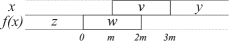
Figure 2: A right stair $(v,w)$ of length $3m$ connecting $y$ and $z$, confirmed by $x$ at position $i=0$.

Definition 14.

Let $f:S^{\mathbb{Z}}\longrightarrow S^{\mathbb{Z}}$ be a cellular automaton, and let $m$ be a positive integer. Let $y\in S^{[i+3m,\infty)}$ be a right infinite word and let $z\in S^{(-\infty,i)}$ be a left-infinite word.

• A pair of words $(v,w)\in S^{2m}\times S^{2m}$ is a right stair connecting $(y,z)$ if there is a configuration $x\in S^{\mathbb{Z}}$ such that $vy=x_{[i+m,\infty)}$ and $zw=f(x)_{(-\infty,i+2m)}$.

• The stair has length $3m$ and it is confirmed (at position $i$) by configuration $x$.

• We write $\Psi_{3m}(y,z)$ for the set of all right stairs of length $3m$ connecting $(y,z)$.

• We write $\Psi_{3m}$ for the union of $\Psi_{3m}(y,z)$ over all $y$ and $z$.

Due to shift invariance, $x$ confirms $(v,w)\in\Psi_{3m}(y,z)$ if and only if $\sigma(x)$ confirms $(v,w)\in\Psi_{3m}(\sigma(y),\sigma(z))$. This means that $\Psi_{3m}(y,z)=\Psi_{3m}(\sigma(y),\sigma(z))$, so it is enough to consider $i=0$ in Definition 14. In terms of cylinders, $(v,w)\in\Psi_{3m}$ if and only if $f([v]_{[m,3m)})\cap[w]_{[0,2m)}\neq\emptyset$.

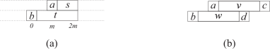
Figure 3: (a) An illustration for Lemma 15, and (b) an illustration for Corollary 16(b) and for Lemma 18.

We need the following known fact concerning left-closing CA. It appears as Proposition 5.44 in [3] where it is stated for right-closing CA. See Figure 3(a) for an illustration.

Lemma 15 (Proposition 5.44 in [3]).

Let $f$ be a left-closing CA. For all sufficiently large $m\in\mathbb{N}$, if $s\in S^{m}$ and $t\in S^{2m}$ are such that $f([s]_{(m,2m]})\cap[t]_{(0,2m]}\neq\emptyset$ then for all $b\in S$ there exists a unique $a\in S$ such that $f([as]_{[m,2m]})\cap[bt]_{[0,2m]}\neq\emptyset$.

The condition $f([s]_{(m,2m]})\cap[t]_{(0,2m]}\neq\emptyset$ is just a way to write that there exists $x\in S^{\mathbb{Z}}$ with $x_{(m,2m]}=s$ and $f(x)_{(0,2m]}=t$. Note that the statement of the lemma has two parts: the existence of $a$ and the uniqueness of $a$. We need both parts in the following.

A number $m$ is a strong left-closing radius for a CA $f$ if it satisfies the claim of Lemma 15, and furthermore $m\geq 2r$ where $r\geq 1$ is a neighborhood radius of $f$. Next we state corollaries of the previous lemma, phrased for right stairs in place of $s$ and $t$ to be directly applicable in our setup.

Corollary 16.

Let $f$ be a left-closing CA. Let $m$ be a strong left-closing radius.

• $\Psi_{3m}(y,z)=\Psi_{3m}$ for all $y$ and $z$.

• Let $(vc,wd)\in\Psi_{3m}$ for $c,d\in S$ and $v,w\in S^{2m-1}$. For every $b\in S$ there exists a unique $a\in S$ such that $(av,bw)\in\Psi_{3m}$. (See Figure 3(b) for an illustration.)

• Every $(v,w)\in\Psi_{3m}(y,z)$ is confirmed by a unique $x$.

Proof.

(a) Let $y,y^{\prime}\in S^{[3m,\infty)}$ and $z,z^{\prime}\in S^{(-\infty,0)}$ be arbitrary. It is enough to prove that $\Psi_{3m}(y^{\prime},z^{\prime})\subseteq\Psi_{3m}(y,z)$. The claim then follows from this and shift invariance $\Psi_{3m}(y,z)=\Psi_{3m}(\sigma(y),\sigma(z))$.

First we show that $\Psi_{3m}(y^{\prime},z^{\prime})\subseteq\Psi_{3m}(y,z^{\prime})$. Let $(v,w)\in\Psi_{3m}(y^{\prime},z^{\prime})$ be arbitrary, so that there exists $x^{\prime}\in[vy^{\prime}]_{[m,\infty)}$ such that $f(x^{\prime})_{(-\infty,2m)}=z^{\prime}w$. Then $(v,w)\in\Psi_{3m}(y,z^{\prime})$ is confirmed by the configuration $x^{\prime\prime}$ such that $x^{\prime\prime}_{(-\infty,3m)}=x^{\prime}_{(-\infty,3m)}$ and $x^{\prime\prime}_{[3m,\infty)}=y$. Indeed, $x^{\prime\prime}_{[m,\infty)}=vy$, and because $m\geq r$, the radius of the local rule of $f$, we also have $f(x^{\prime\prime})_{(-\infty,2m)}=f(x^{\prime})_{(-\infty,2m)}=z^{\prime}w$.

Next we show that $\Psi_{3m}(y,z^{\prime})\subseteq\Psi_{3m}(y,z)$. Let $(v,w)\in\Psi_{3m}(y,z^{\prime})$. We start with finite extensions of $w$ on the left: we prove that for every finite word $u\in S^{*}$ we have $f([vy]_{[m,\infty)})\cap[uw]_{[-|u|,2m)}\neq\emptyset$. Suppose the contrary, and let $bu\in S^{k+1}$ be the shortest counterexample, with $b\in S$ and $u\in S^{k}$. (By the assumptions, the empty word is not a counterexample.) By the minimality of $bu$, there exists $x^{r}\in[vy]_{[m,\infty)}$ such that $f(x^{r})_{[-k,2m)}=uw$. Choose $s=x^{r}_{[-k+m,-k+2m)}$ and $t=f(x^{r})_{[-k,-k+2m)}$ and apply the existence part of Lemma 15. By the lemma, there exists a configuration $x^{l}$ such that $x^{l}_{[-k+m,-k+2m)}=x^{r}_{[-k+m,-k+2m)}$ and $f(x^{l})_{[-k-1,-k+2m)}=b\cdot f(x^{r})_{[-k,-k+2m)}$.

Consider $x$ obtained by gluing together the left half of $x^{l}$ and the right half of $x^{r}$: define $x_{(-\infty,-k+2m)}=x^{l}_{(-\infty,-k+2m)}$ and $x_{[-k+m,\infty)}=x^{r}_{[-k+m,\infty)}$. Note that in the region $[-k+m,-k+2m)$ configurations $x^{l}$ and $x^{r}$ have the same value. By applying the local rule of $f$ with radius $r$ we also get that $f(x)_{(-k-1,-k+2m-r)}=f(x^{l})_{(-k-1,-k+2m-r)}=b\cdot f(x^{r})_{[-k,-k+2m-r)}$ and $f(x)_{[-k+m+r,2m)}=f(x^{r})_{[-k+m+r,2m)}$. Because $m\geq 2r$ we have $-k+2m-r\geq-k+m+r$, so that $f(x)_{(-k-1,2m)}=b\cdot f(x^{r})_{(-k,2m)}=buw$. We also have $x_{[m,\infty)}=x^{r}_{[m,\infty)}=vy$, so that $x$ proves that $bu$ is not a counterexample.

Consider then the infinite extension of $w$ on the left by $z$: Applying the finite case above to each finite suffix of $z$ and by taking a limit, we see with a simple compactness argument that there exists $x\in[vy]_{[m,\infty)}$ such that $f(x)_{[-\infty,2m)}=zw$. This proves that $(v,w)\in\Psi_{3m}(y,z)$.

(b) Let $(vc,wd)\in\Psi_{3m}$ and let $b\in S$ be arbitrary. Let $y\in S^{[3m,\infty)}$ be arbitrary, and and let $z\in S^{(-\infty,0)}$ be such that $z_{-1}=b$. By (a) we have that $(vc,wd)\in\Psi_{3m}(y,z)$. Let $x$ be a configuration that confirms this, so $x_{[m,\infty)}=vcy$ and $f(x)_{(-\infty,2m)}=zwd$. Let $a=x_{m-1}$. Because $x_{[m-1,3m-1)}=av$ and $f(x)_{[-1,2m-1)}=bw$, configuration $x$ confirms (at position $i=-1$) that $(av,bw)\in\Psi_{3m}$.

Let us prove that $a$ is unique. Suppose that also $(a^{\prime}v,bw)\in\Psi_{3m}$. We apply the uniqueness part of Lemma 15 on $s$ and $t$ where $t=wd$ and $s$ is the prefix of $v$ of length $m$. Because $(a^{\prime}v,bw)$ is a right stair, $f([a^{\prime}v]_{[m-1,3m-1)})\cap[bw]_{[-1,2m-1)}\neq\emptyset$. Because $m-1\geq 2r-1\geq r$, the local rule of $f$ assigns $f(x)_{2m-1}=d$ for all $x\in[a^{\prime}v]_{[m-1,3m-1)}$, so that $f([a^{\prime}v]_{[m-1,3m-1)})\cap[bwd]_{[-1,2m)}\neq\emptyset$. But then $f([a^{\prime}s]_{[m-1,2m)})\cap[bt]_{[-1,2m)}\neq\emptyset$, so that by Lemma 15 we must have $a^{\prime}=a$.

(c) Suppose $x\neq x^{\prime}$ both confirm that $(v^{\prime},w^{\prime})\in\Psi_{3m}(y,z)$. Then $x_{[m,\infty)}=v^{\prime}y=x^{\prime}_{[m,\infty)}$. Let $k<m$ be the largest index such that $x_{k}\neq x^{\prime}_{k}$. Extract $a,a^{\prime},b,c,d\in S$ and $v,w\in S^{2m-1}$ from $x$ and $x^{\prime}$ as follows: $avc=x_{[k,k+2m]}$ and $a^{\prime}vc=x^{\prime}_{[k,k+2m]}$ and $bwd=f(x)_{[k-m,k+m]}=f(x^{\prime})_{[k-m,k+m]}$. Then $(vc,wd)\in\Psi_{3m}$ and $(av,bw),(a^{\prime}v,bw)\in\Psi_{3m}$. This contradicts (b). ∎

Now we can prove another constraint on sliders.

Lemma 17.

Let $f$ be a slider. Let $m$ be a strong left-closing radius, and big enough so that $f$ is defined by a bijective block rule $\chi:S^{n}\longrightarrow S^{n}$ of block length $n=3m$. Let $N$ be the number of representatives of configurations (independent of the configuration) with respect to $\chi$. Then

$$N\cdot|\Psi_{n}|=|S|^{n}.$$

In particular, $|\Psi_{n}|$ divides $|S|^{n}$.

Proof.

Fix any $y\in S^{[3m,\infty)}$ and $z\in S^{(-\infty,0)}$. Denote $A=\{x\in S^{\mathbb{Z}}\ |\ x_{[3m,\infty)}=y\mbox{ and }f(x)_{(-\infty,0)}=z\}$. Consider the function $A\longrightarrow\Psi_{3m}(y,z)$ defined by $x\mapsto(x_{[m,3m)},f(x)_{[0,2m)})$. It is surjective by the definition of $\Psi_{3m}(y,z)$, and it is injective by Corollary 16(c). Because $\Psi_{3m}(y,z)=\Psi_{3m}$ by Corollary 16(a), we see that $|A|=|\Psi_{3m}|$.

For each $w\in S^{3m}$ define configuration $x^{w}=zwy$. Representations $(x,0)$ of $y\in A$ are precisely $(x^{w},0)$ for $w\in S^{3m}$. Because each $y$ has $N$ representations and there are $|S|^{3m}$ words $w$ we obtain that $N\cdot|\Psi_{3m}|=|S|^{3m}$. ∎

Now we prove the converse: the constraints we have proved for sliders are sufficient. This completes the characterization of sliders.

Lemma 18.

Let $f$ be a left-closing cellular automaton, let $m$ be a strong left-closing radius, and assume that $|\Psi_{n}|$ divides $|S|^{n}$ for $n=3m$. Then $f$ is a slider.

Proof.

Let $N=|S|^{n}/|\Psi_{n}|$ and pick an arbitrary bijection $\pi:\Psi_{n}\times\{1,2,\dots,N\}\longrightarrow S^{n}$. Let $f_{\mathrm{loc}}:S^{2m+1}\longrightarrow S$ be the local rule of radius $m$ for the cellular automaton $f$.

Let us define a block rule $\chi:S^{n+1}\longrightarrow S^{n+1}$ as follows (see Figure 3). Consider any $c\in S$, any $k\in\{1,2,\dots,N\}$ and any $(av,bw)\in\Psi_{n}$ where $a,b\in S$ and $v,w\in S^{2m-1}$. Let $d=f_{\mathrm{loc}}(avc)$. We set $\chi:\pi((av,bw),k)\cdot c\mapsto b\cdot\pi((vc,wd),k))$. This completely defines $\chi$, but to see that it is well defined we next show that $(vc,wd)$ is a right stair. By Corollary 16(a) we have that $(av,bw)\in\Psi_{n}(cy,z)$ for arbitrary $y,z$ so there is a configuration $x$ such that $x_{[m,\infty)}=avcy$ and $f(x)_{(\infty,2m)}=zbw$. The local rule $f_{\mathrm{loc}}$ determines that $f(x)_{2m}=f_{\mathrm{loc}}(avc)=d$. It follows that $(vc,wd)\in\Psi_{n}(y,zb)$, confirmed by $x$ at position $i=1$.

Now that we know that $\chi$ is well defined, let us prove that $\chi$ is a bijection. Suppose $\pi((av,bw),k)\cdot c$ and $\pi((a^{\prime}v^{\prime},b^{\prime}w^{\prime}),k^{\prime})\cdot c^{\prime}$ have the same image $b\cdot\pi((vc,wd),k))=b^{\prime}\cdot\pi((v^{\prime}c^{\prime},w^{\prime}d^{\prime}),k^{\prime}))$. We clearly have $b=b^{\prime}$, and because $\pi$ is a bijection, we have $v=v^{\prime}$, $c=c^{\prime}$, $w=w^{\prime}$, $d=d^{\prime}$ and $k=k^{\prime}$. By Corollary 16(a) we also have that $a=a^{\prime}$.

As $\chi$ is a bijective block rule, it defines a slider relation $F$. We need to prove that for every configuration $y$, the only $z$ such that $(y,z)\in F$ is $z=f(y)$. Therefore, consider an arbitrary representation $(x,i)$ of $(y,z)\in F$. Write $x=z_{(-\infty,i)}\cdot\pi((av,bw),k)\cdot c\cdot y_{[i+n+1,\infty)}$ for letters $a,c,b\in S$ words $v,w\in S^{2m-1}$ and $k\in\{1,2,\dots,N\}$. This can be done and as $\pi$ is surjective and all items in this representation are unique as $\pi$ is injective. We have $(av,bw)\in\Psi_{n}(cy,z)$ so by Corollary 16(c) there is a unique configuration $x^{\prime}$ that confirms this. Then $x^{\prime}_{[i+m,\infty)}=avc\cdot y_{[i+n+1,\infty)}$ and $f(x^{\prime})_{(-\infty,i+2m)}=z_{(-\infty,i)}\cdot bw$. Associate $x^{\prime}$ to $(x,i)$ by defining $g(x,i)=x^{\prime}$.

Let us show that $g(\chi^{i}(x),i+1)=g(x,i)$. By the definition of $\chi$ we have

$$\chi^{i}(x)=z_{(-\infty,i)}\cdot b\cdot\pi((vc,wd),k))\cdot y_{[i+n+1,\infty)}$$

where $d=f_{\mathrm{loc}}(avc)$. To prove that $g(\chi^{i}(x),i+1)=x^{\prime}=g(x,i)$ it is enough to show that $x^{\prime}$ confirms $(vc,wd)\in\Psi_{n}(y,zb)$. But this is the case because $x^{\prime}_{[i+m+1,\infty)}=vc\cdot y_{[i+n+1,\infty)}$ and $f(x^{\prime})_{(-\infty,i+2m+1)}=z_{(-\infty,i)}\cdot bwd$. The fact that $f(x^{\prime})_{i+2m}=d$ follows from $x^{\prime}_{[i+m,i+3m]}=avc$ and $d=f_{\mathrm{loc}}(avc)$.

By induction we have that for any $j\geq i$ holds $g(\chi^{[i,j)}(x),j)=x^{\prime}$. Moreover, pair $(\chi^{[i,j)}(x),j)$ represents the same $(y,z)\in F$ as $(x,i)$. Therefore, $x^{\prime}_{[j+n+1,\infty)}=y_{[j+n+1,\infty)}$ and $f(x^{\prime})_{(-\infty,j)}=z_{(-\infty,j)}$ for all $j\geq i$. Let us look into position $p=i+n+m+1$. Using any $j>p$ we get $f(x^{\prime})_{p}=z_{p}$ and using $j=i$ we get $x^{\prime}_{[p-m,p+m]}=y_{[p-m,p+m]}$. This means that $z_{p}=f_{\mathrm{loc}}(y_{[p-m,p+m]})$, that is, $z_{p}=f(y)_{p}$. Because $i$ was arbitrary, $p$ is arbitrary. We have that $z=f(y)$, which completes the proof. ∎

Theorem 19.

The function $f$ admits a slider if and only if $f$ is a left-closing cellular automaton and $|\Psi_{n}|$ divides $|S|^{n}$ for $n=3m$ where $m$ is the smallest strong left-closing radius.

We can state this theorem in a slightly more canonical (but completely equivalent) form by normalizing the length of stairs:

By Corollary 16, for a left-closing cellular automaton $f$ the limit

$$\lambda_{f}=\lim_{m\to\infty}\frac{|\Psi_{3m}|}{|S|^{3m}}$$ (2)

is reached in finite time, namely as soon as $m$ is a left-closing radius, and thus $\lambda_{f}$ is rational for left-closing $f$. In [2] it is shown that the map $f\mapsto\lambda_{f}$ gives a homomorphism from the group of reversible cellular automata into the rational numbers under multiplication. For a prime number $p$ and an integer $n$, write $v_{p}(n)$ for the largest exponent $k$ such that $p^{k}|n$. For prime $p$ and rational $r=m/n$, write $v_{p}(r)=v_{p}(m)-v_{p}(n)$ for the $p$-adic valuation of $r$.

Theorem 20.

The function $f$ is a slider if and only if $f$ is a left-closing cellular automaton and $v_{p}(\lambda_{f})\leq 0$ for all primes $p$.

Example 21.

Let $A=\{0,1\}\times\{0,1,2\}$ and write $\sigma_{2}$ and $\sigma_{3}$ for the left shifts on the two tracks of $A^{\mathbb{Z}}$. Then consider $f=\sigma_{2}\times\sigma_{3}^{-1}$. For this CA we have by a direct computation $|\Psi_{3}|=2^{2}\cdot 3^{4}$ so $\lambda_{f}=2^{2}\cdot 3^{4}/6^{3}$ so $v_{3}(\lambda_{f})=1>0$, and thus $f$ is not a slider. Similarly we see that $\sigma_{3}\times\sigma_{2}^{-1}$ is not a slider.

Example 22.

Let $S=\{0,1\}$ and consider the exclusive-or CA with neighborhood $\{-1,0\}$, i.e. $f(x)=x+\sigma^{-1}(x)$. Then $f$ is left-closing but a direct computation shows $v_{2}(\lambda_{f})=1>0$, so $f$ is not a slider. Compare with Example 4.

2.3 Definition of sweepers

An alternative approach not requiring bijectivity of $\chi$ is specified in the following:

Definition 23.

A block rule $\chi$ defines a sweeper relation $F\subset S^{\mathbb{Z}}\times S^{\mathbb{Z}}$ by $(y,z)\in F$ iff some subsequence of $\chi^{0+}(y),\chi^{-1+}(y),\chi^{-2+}(y),\dots$ converges to $z$.

Lemma 24.

The projection $(y,z)\mapsto y$ on the first component maps a sweeper relation $F$ surjectively onto $S^{\mathbb{Z}}$. The relation $F$ is a function $f$ if and only if for each configuration $y$ the limit $\lim_{i\to-\infty}{\chi}^{i+}(y)$ exists and equals $f(y)$.

Proof.

For every $y\in S^{\mathbb{Z}}$ the sequence $\chi^{0+}(y),\chi^{-1+}(y),\chi^{-2+}(y),\dots$ has a converging subsequence with some limit $z$. Then $(y,z)\in F$ so the projection is onto.

If $z=\lim_{i\to-\infty}{\chi}^{i+}(y)$ exists then every subsequence of $\chi^{0+}(y),\chi^{-1+}(y),\chi^{-2+}(y),\dots$ converges to $z$ so $z$ is the unique configuration such that $(y,z)\in F$. Conversely, if $\lim_{i\to-\infty}{\chi}^{i+}(y)$ does not exist then $\chi^{0+}(y),\chi^{-1+}(y),\chi^{-2+}(y),\dots$ has two subsequences converging to distinct $z_{1}$ and $z_{2}$. In this case $(y,z_{1})$ and $(y,z_{2})$ are both in relation $F$. ∎

Definition 25.

Let $\chi$ be a block rule such that for each configuration $y$ the limit $z=\lim_{i\to-\infty}{\chi}^{i+}(y)$ exists. The function $y\mapsto z$ is called the sweeper defined by $\chi$.

Before we are going to compare the notions of sliders and sweepers we provide a result on a special kind of Mealy automata.

2.4 A note on finite Mealy automata

In this section we consider Mealy automata with a set $Q$ of states and where the set $A$ of input symbols and the set of output symbols coincide. For convenience instead of pairs of elements we use words of length $2$. Thus, we denote by $\mu:QA\to AQ$ the function mapping the current state $q$ and an input symbol $a$ to $\mu(qa)=a^{\prime}q^{\prime}$, where $q^{\prime}$ is the new state of the automaton.

The motivation for this is the following. When a block rule $\chi$ is sweeping over a configuration one can think of the block $q\in S^{n}$ where $\chi$ will be applied next as encoding the state of a Mealy automaton. The word $a\in S^{n}$ immediately to the right of it is the next input symbol. By applying $\chi$ at positions $0,1,\dots,n-1$ the word $qa$ is transduced into a word $a^{\prime}q^{\prime}\in S^{2n}$ where $a^{\prime}$ can be considered the output symbol and $q^{\prime}$ the next state of the automaton. When $\chi$ is bijective then clearly $\mu$ is bijective, too.

Let $\delta:QA\to Q$ denote the function yielding only the new state of the Mealy automaton. The extension $\delta^{*}:QA^{*}\to A^{*}Q$ to input words is for all states $q$, all inputs $w\in A^{*}$ and $a\in A$ defined by $\delta^{*}(q\varepsilon)=q$ and $\delta^{*}(qwa)=\delta(\delta^{*}(qw)a)$.

Because of the application we have in mind we now restrict ourselves to the case where $Q=A$ and speak of elements $e\in Q$. Let $\bar{e}=(\ldots,e_{-2},e_{-1},e_{0})$ denote a sequence of elements which is infinite to the left.

Definition 26.

A finite tail $\bar{e}_{i}=(e_{-i},\ldots,e_{0})$ of $\bar{e}$ is good for $q$ if $\delta^{*}(\bar{e}_{i})=q$. An infinite sequence $\bar{e}$ is good for $q$ if infinitely many finite tails $\bar{e}_{i}=(e_{-i},\ldots,e_{0})$ are good for $q$.

A state $q$ is good, if there is an infinite sequence $\bar{e}$ that is good for $q$. Let $G\subseteq Q$ denote the set of good states and $B\subseteq Q$ the set of bad states.

Lemma 27.

If $\mu$ is bijective then $G=Q$ and $B=\emptyset$.

Proof.

First, observe that the property of being good is preserved by $\delta$. If $g$ is good, then each $\delta(ga)$ is good, too: If $\bar{e}$ is good for $g$, then $\bar{e}a$ is good for $\delta(ga)$ since $\delta^{*}(e_{-i},\ldots,e_{0})=g$ implies $\delta^{*}(e_{-i},\ldots,e_{0},a)=\delta(ga)$. This means that $\mu(GA)\subseteq AG$.

Since $\mu$ is injective and $|GA|=|AG|$, in fact $\mu(GA)=AG$. Therefore $\mu(BA)\subseteq AB$, that is $\delta$ preserves bad states. Now, assume that there indeed exists a bad state $b\in B$. Consider $\bar{b}=(\ldots,b,b,b)$. The states $b_{i}=\delta^{*}(b^{i})$ are all bad, but at least one of them happens infinitely often, which would mean that it is good. Contradiction. ∎

2.5 Relation between sliders and sweepers

Compared to definition 10 the advantage of definition 25 is that it does not require $\chi$ to be bijective. But as long as $\chi$ is bijective, there is in fact no difference.

Theorem 28.

Let $\chi$ be a bijective block rule and $f$ a one-dimensional CA. The slider relation defined by $\chi$ is equal to $f$ if and only if the sweeper relation it defines is equal to $f$.

The two implications are considered separately in Lemmata 29 and 30 below. For the remainder of this section let $\chi:S^{n}\to S^{n}$ always denote a bijective block rule and let $f:S^{\mathbb{Z}}\to S^{\mathbb{Z}}$ denote a one-dimensional CA (without stating this every time).

Lemma 29.

If $\chi$ is not a sweeper for $f$ then it is not a slider for $f$.

Proof.

If $\chi$ is not a sweeper for $f$ then there is a configuration $y$ for which the limit $\lim_{i\to-\infty}\chi^{[i,\infty)}(y)$ does not exist or is wrong. In both cases there is a cell $j\in\mathbb{Z}$ and a state $s\in S$ such that $s\not=f(y)_{j}$ but $\chi^{[i,\infty)}(y)_{j}=s$ for infinitely many $i<j-n$.

We will construct a configuration $x$ such that $\chi^{j-}(x)=y$ and $\chi^{j+}(x)_{j}=s\not=f(y)_{j}$. Therefore $\chi$ is not a slider for $f$ (see Def. 10).

As a first step we subdivide the “left part” $(-\infty,j+n)$ of $\mathbb{Z}$ into windows $W_{k}$ of length $n$. For $k\geq 0$ let $p_{k}=-kn+j$ denote the smallest index in $W_{k}$, i. e. $W_{k}=[p_{k},p_{k-1})$ (where $p_{-1}=j+n$). Analogously divide the “left part” of $y$ into words $y^{(k)}$ of length $n$ by setting $y^{(k)}=y|_{W_{k}}$ (see Fig. 4).

Figure 4: For configuration $y$ the windows $W_{k}$ contain the words $y^{(k)}$.

Let $M$ denote the set $\{i\mid\chi^{[i,\infty)}(y)_{j}=s\}$. $M$ contains infinitely many integers $i<p_{1}=j-n$. Then there has to be a word $v^{(0)}\in S^{n}$ such that the set $M_{0}=\{i\in M\mid i<p_{1}\text{ and }\chi^{[i,j)}(y)|_{W_{0}}=v^{(0)}\}$ is infinite. Since $M_{0}\subseteq M$ certainly $\chi(v^{(0)})_{0}=s$ holds.

Figure 5: Transition from $v^{(k+1)}y^{(k)}$ to $x^{(k+1)}v^{(k)}$ by applying $\chi$ from left to right at the positions indicated by the gray bars. Application of the inverse $\xi$ from right to left realizes the opposite transition from bottom to top.

For all $k\geq 0$ we now inductively define words $v^{(k+1)}$ and $x^{(k+1)}$ (all of length $n$) and along with it infinite sets $M_{k+1}$. Since $M_{k}$ is infinite, there is a word $v^{(k+1)}$ such that the set

$$M_{k+1}=\{i\in M_{k}\mid i<p_{k+2}\text{ and }\chi^{[i,p_{k})}(y)|_{W_{k+1}}=v^{(k+1)}\}$$

is infinite. Since $M_{k+1}\subseteq M_{k}$ one has $\chi^{[p_{k+1},p_{k})}(v^{(k+1)}y^{(k)})=x^{(k+1)}v^{(k)}$ for some $x^{(k+1)}$ (see Fig.5). Since $\chi$ is bijective, for the inverse $\xi$ of $\chi$ holds $v^{(k+1)}y^{(k)}=\xi^{[p_{k+1},p_{k})^{R}}(x^{(k+1)}v^{(k)})$, too. Note again that $\xi$ is applied from right to left.

Now choose configuration $x=\cdots x^{(3)}\cdot x^{(2)}\cdot x^{(1)}\cdot v^{(0)}\cdot y_{[j+n,\infty)}$.

On one hand $\chi^{j+}(x)$ already after the application of $\chi$ at position $j$ produces state $s$ there which never changes again. Thus $\chi^{j+}(x)\not=f(y)$.

On the other hand by construction for all $k\geq 0$ holds $\xi^{[p_{k+1},p_{k})^{R}}(x^{(k+1)}v^{(k)})=v^{(k+1)}y^{(k)}$. Therefore

$$\xi^{[p_{1},p_{0})^{R}}(x) =\xi^{[p_{1},p_{0})^{R}}(\cdots x^{(3)}x^{(2)}x^{(1)}v^{(0)}y_{[j+n,\infty)})$$

$$=\cdots x^{(3)}x^{(2)}v^{(1)}z^{(0)}y_{[j+n,\infty)}$$

and by induction for all $$k\geq 0$$

$$\xi^{[p_{k+1},p_{0})^{R}}(x) =\xi^{[p_{k+1},p_{0})^{R}}(\cdots x^{(3)}x^{(2)}x^{(1)}v^{(0)}y_{[j+n,\infty)})$$

$$=\cdots x^{(k+1)}v^{(k)}y^{(k-1)}\cdots y^{(0)}y_{[j+n,\infty)}$$

Obviously one gets ${\xi}^{i-}(x)=y$. ∎

Lemma 30.

If $\chi$ is not a slider for $f$ then it is not a sweeper for $f$.

Proof.

If $\chi$ is not a slider for $f$ then there exists a configuration $x$ and an $i\in\mathbb{Z}$ such that for $z={\chi}^{i+}(x)$ and $y={\chi}^{i-}(x)$ one has $f(y)\not=z$. Let $\xi$ be the inverse of $\chi$. Let $j$ be a cell where $f(y)_{j}\not=z_{j}$. If $j<i+n$ instead of $x$ can consider $x^{\prime}=\xi^{[i-1,\dots,i-m]}(x)$ for some sufficiently large $m$. Assume therefore that $j\geq i+n$.

We will prove that there is a configuration $v$ such that for infinitely many positions $m$ the configuration $\chi^{[m,\infty)}(v)$ will not have the correct state at position $j$. Therefore the limit $\lim_{m\to-\infty}\chi^{[m,\infty)}(v)$ cannot exist and have the correct state at position $j$. Thus $\chi$ is not a sweeper for $f$.

Below the abbreviation $Q=S^{n}$ is used.

Configuration $x$ is of the form $z_{(-\infty,i)}\cdot w\cdot y_{[i+n,\infty)}$ for some $w\in Q$. Applying $\chi$ at position $i$ and further to the right produces the same result independent of what is to the left of $w$. Therefore if $z_{(-\infty,i)}$ is replaced by any $z^{\prime}_{(-\infty,i)}$ still the wrong state is produced at position $j$.

Define a Mealy automaton with $Q=A$ by $\mu(qa)=\chi^{[0,n)}(qa)$ (observe that $qa\in S^{2n}$). Since $\mu$ is bijective, one can now use the result from Lemma 27 and conclude that there is a sequence $(\ldots,v^{(2)},v^{(1)})$, infinite to the left, of elements $v^{(k)}\in Q$ such that

$$\delta^{*}(v^{(k)}\cdots v^{(1)})=w k$$ for infinitely many . (3)

Let $v$ be the infinite to the left half-configuration obtained by concatenating all $v^{(k)}$, more precisely $v:(-\infty,i+n)\to S$ where $v_{-kn+j+i}=v^{(k)}_{j}$ for all $k\geq 1$ and all $j\in[0,n)$.

Condition (3) implies that for infinitely many $k\geq 1$ applying $\chi$ in $v$ from position $-kn+i$ up to but excluding $i$ produces $w$ at the end, i. e. in the window $[i,i+n)$. In other words $\chi^{[-kn+i,i)}(v)=v^{\prime}_{(-\infty,i)}\cdot w$ ($v^{\prime}$ depends on $k$ but doesn’t matter). Therefore for infinitely many $k$

$$\chi^{[-kn+i,i)}(vy_{[i+n,\infty)}) =\cdots\cdot w\cdot z_{[i+n,\infty)}$$

$$\text{and \quad}\chi^{[-kn+i,\infty)}(vy_{[i+n,\infty)}) =\cdots\cdot w^{\prime}\cdot z_{[i+n,\infty)}$$

Since we could assume that the position $j$ where $f(y)_{j}\not=z_{j}$ is in the interval $[i+n,\infty)$ one can conclude that $\chi$ is not a sweeper for $f$. ∎

While the slider and sweeper relations defined by a block rule are equal when at least one them defines a cellular automaton, sweeper relations can also define non-continuous functions.

Example 31.

Let $S=\{\left[\begin{smallmatrix}0\\ 0\end{smallmatrix}\right],\left[\begin{smallmatrix}0\\ 1\end{smallmatrix}\right],\left[\begin{smallmatrix}1\\ 0\end{smallmatrix}\right],\left[\begin{smallmatrix}1\\ 1\end{smallmatrix}\right]\}$ and define $\chi:S^{2}\to S^{2}$ by $\chi(\left[\begin{smallmatrix}1\\ 0\end{smallmatrix}\right]\left[\begin{smallmatrix}0\\ 0\end{smallmatrix}\right])=\left[\begin{smallmatrix}0\\ 0\end{smallmatrix}\right]\left[\begin{smallmatrix}0\\ 1\end{smallmatrix}\right]$, $\chi(\left[\begin{smallmatrix}0\\ 0\end{smallmatrix}\right]\left[\begin{smallmatrix}0\\ 1\end{smallmatrix}\right])=\left[\begin{smallmatrix}1\\ 0\end{smallmatrix}\right]\left[\begin{smallmatrix}0\\ 0\end{smallmatrix}\right]$, and $\chi(ab)=ab$ for $ab\notin\{\left[\begin{smallmatrix}1\\ 0\end{smallmatrix}\right]\left[\begin{smallmatrix}0\\ 0\end{smallmatrix}\right],\left[\begin{smallmatrix}0\\ 0\end{smallmatrix}\right]\left[\begin{smallmatrix}0\\ 1\end{smallmatrix}\right]\}$.

We claim that $\lim_{i\rightarrow-\infty}\chi^{i+}(x)$ is well-defined for all $x\in S^{\mathbb{Z}}$, so that the sweeper relation $\chi$ defines is a function. Let $x\in S^{\mathbb{Z}}$ be arbitrary, and let $n\in\mathbb{Z}$. We need to show that $\chi^{i+}(x)_{n}$ converges.

Suppose first that for some $k<n$, we have $x_{k}=\left[\begin{smallmatrix}1\\ a\end{smallmatrix}\right]$ for $a\in\{0,1\}$. Then for all $i<k$, the value $\chi^{i+}(x)_{n}$ is independent of the values $x_{j}\leq k$, since $\chi^{[i,k-1]}(x)_{k}=\left[\begin{smallmatrix}1\\ a\end{smallmatrix}\right]$, meaning that the sweep is synchronized (in the sense that whatever information was coming from the left is forgotten and the sweep continues the same way) and $\chi^{i+}(x)_{n}$ is determined by $x_{[k,n]}$ for all $i<k$. Thus, in this case $\chi^{i+}(x)_{n}$ converges.

Suppose then that for all $k<n$, $x_{k}=\left[\begin{smallmatrix}0\\ a\end{smallmatrix}\right]$ for some $a\in\{0,1\}$. If $x_{k}=\left[\begin{smallmatrix}0\\ 0\end{smallmatrix}\right]$ for some $k<n$, then since $x_{k-1}\neq\left[\begin{smallmatrix}1\\ 0\end{smallmatrix}\right]$ we also have $\chi^{[i,k-2]}(x)_{k-1}\neq\left[\begin{smallmatrix}1\\ 0\end{smallmatrix}\right]$. Thus, the value at $k$ does not change when $\chi$ is applied at $k-1$, and as in the previous paragraph, the sweep is synchronized at this position. Again $\chi^{i+}(x)_{n}$ is determined by $x_{[k,n]}$ for all $i<k$, so $\chi^{i+}(x)_{n}$ converges.

In the remaining case, $x_{k}=\left[\begin{smallmatrix}0\\ 1\end{smallmatrix}\right]$ for all $k<n$. Then since $\chi(\left[\begin{smallmatrix}0\\ 1\end{smallmatrix}\right]\left[\begin{smallmatrix}0\\ 1\end{smallmatrix}\right])=\left[\begin{smallmatrix}0\\ 1\end{smallmatrix}\right]\left[\begin{smallmatrix}0\\ 1\end{smallmatrix}\right]$, the rule is not applied in the left tail of $x$, and thus certainly $\chi^{i+}(x)_{n}$ converges.

The function defined by the sweeper relation is not continuous at $\left[\begin{smallmatrix}0\\ 1\end{smallmatrix}\right]^{\mathbb{Z}}$ since $\chi^{\mathbb{Z}}(\left[\begin{smallmatrix}0\\ 1\end{smallmatrix}\right]^{\mathbb{Z}})=\left[\begin{smallmatrix}0\\ 1\end{smallmatrix}\right]^{\mathbb{Z}}$ while for any $n\in\mathbb{N}$ we have

$$\chi^{\mathbb{Z}}(...\left[\begin{smallmatrix}0\\ 0\end{smallmatrix}\right]\left[\begin{smallmatrix}0\\ 0\end{smallmatrix}\right]\left[\begin{smallmatrix}0\\ 0\end{smallmatrix}\right]\left[\begin{smallmatrix}0\\ 1\end{smallmatrix}\right]^{n}.\left[\begin{smallmatrix}0\\ 1\end{smallmatrix}\right]^{\mathbb{N}})=...\left[\begin{smallmatrix}0\\ 0\end{smallmatrix}\right]\left[\begin{smallmatrix}0\\ 0\end{smallmatrix}\right]\left[\begin{smallmatrix}1\\ 0\end{smallmatrix}\right]\left[\begin{smallmatrix}1\\ 0\end{smallmatrix}\right]^{n}.\left[\begin{smallmatrix}1\\ 0\end{smallmatrix}\right]^{\mathbb{N}}$$

3 Realization of bi-closing CA using LR and RL sliders

In the definition of a slider we use a left-to-right slide of the window to realize the CA transition. Of course, one can analogously define right-to-left sliders and prove a characterization via right-closing CA. We can also alternate these two types of rules, and obtain a ladder-shaped hierarchy analogous to the Borel, arithmetic and polynomial hierarchies.

Definition 32.

Let $\mathcal{R}$ denote the set of CA definable as slider relations with the “from left to right” as in Definition 10. Analogously let $\mathcal{L}$ denote the set of CA definable as right-to-left slider relations. Denote $\Delta=\mathcal{L}\cap\mathcal{R}$. Let now $\mathcal{L}_{0}=\mathcal{R}_{0}=\{\mathrm{id}\}$, and for all $k\in\mathbb{N}_{0}$ let $\mathcal{L}_{k+1}=\mathcal{L}\circ\mathcal{R}_{k}$ and $\mathcal{R}_{k+1}=\mathcal{R}\circ\mathcal{L}_{k}$. For all $n$, write $\Delta_{n}=\mathcal{L}_{n}\cap\mathcal{R}_{n}$.

Note that in $\mathcal{L}_{n}$, there are $n$ sweeps (slider applications) in total, and the last sweep goes from right to left. We have $\mathcal{L}_{1}=\mathcal{L}$, $\mathcal{R}_{1}=\mathcal{R}$, $\Delta_{1}=\Delta$. See Figure 6.

Figure 6: The sliding hierarchy.

In Theorem 35 below we will show a close relation between this “slider hierarchy” and a “closingness hierarchy” defined as follows, exactly analogously. Let $\mathcal{L}^{cl}$ denote the set of left-closing CA and $\mathcal{R}^{cl}$ the set of right-closing CA. Define $\mathcal{L}^{cl}_{0}=\mathcal{R}^{cl}_{0}=\{\mathrm{id}\}$ and for all $k$, $\mathcal{L}^{cl}_{k+1}=\mathcal{L}^{cl}\circ\mathcal{R}^{cl}_{k}$ and $\mathcal{R}^{cl}_{k+1}=\mathcal{R}^{cl}\circ\mathcal{L}^{cl}_{k}$.

As always with such hierarchies, it is natural to ask whether they are infinite or collapse at some finite level. We do not know if either hierarchy collapses, but we show that after the first level, the hierarchies coincide. The main ingredients for the theorem are the following two lemmata.

Lemma 33.

Let $f$ be a left-closing CA. For all $n$ large enough, $|\Psi_{n}|$ divides some power of $|S|$.

Proof.

Let $m$ be a strong left-closing radius for $f$. Number $m$ can be chosen as large as needed. Let $f_{\mathrm{loc}}$ be the local update rule of $f$ of radius $3m$. By Theorem 14.7 in [1] there exist, for $k=3m$ chosen sufficiently large,

• positive integers $L,M$ and $R$ such that $L\cdot M\cdot R=|S|^{2k}$,

• pairwise different words $u_{1},\dots,u_{M}$ of length $k$,

• sets ${\cal L}_{1},\dots,{\cal L}_{M}\subseteq S^{2k}$ of words of length $2k$, each of cardinality $|{\cal L}_{i}|=L$,

• sets ${\cal R}_{1},\dots,{\cal R}_{M}\subseteq S^{2k}$ of words of length $2k$, each of cardinality $|{\cal R}_{i}|=R$,

• a word $w$ of length $3k$ whose set pre-images of length $5k$ under $f_{\mathrm{loc}}$ is precisely

  $$\bigcup_{i=1}^{M}{\cal L}_{i}u_{i}{\cal R}_{i}.$$

See Figure 7 for an illustration.

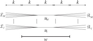
Figure 7: Illustration of Theorem 14.7 in [1], with $L=4$, $R=3$.

Let $y\in S^{[k,\infty)}$ be arbitrary and let $z\in S^{(-\infty,0)}$ be such that $z_{[-3k,0)}=w$. Define $A=\{x\in S^{\mathbb{Z}}\ |\ x_{[k,\infty)}=y,f(x)_{(-\infty,0)}=z\}$. By Corollary 16 we know that $|\Psi_{3m}|=|A|$.

(i) If $x\in A$ then $x_{[-4k,k)}$ is a pre-image of $w=z_{[-3k,0)}$. This means that for some $i\in\{1,\dots,M\}$, we have $x_{[-4k,k)}\in{\cal L}_{i}u_{i}{\cal R}_{i}$ and, in particular, $x_{[-2k,k)}\in u_{i}{\cal R}_{i}$.

(ii) Conversely, let $i\in\{1,\dots,M\}$ and $v\in{\cal R}_{i}$ be arbitrary. Words in ${\cal L}_{i}u_{i}v$ are pre-images of $w$ so $f([u_{i}v]_{[-2k,k)})\cap[w]_{[-3k,0)}\neq\emptyset$. Because $f$ is left-closing and $k$ is a strong left-closing radius for $f$ there exists a unique $x\in A$ such that $x_{[-2k,k)}=u_{i}v$.

From (i) and (ii) we can conclude that $|A|=M\cdot R$. Hence $L\cdot|\Psi_{3m}|=L\cdot|A|=L\cdot M\cdot R=|S|^{2k}$. ∎

Lemma 34.

Let $f$ be a left-closing CA. Then for any large enough $n$, we have $\sigma^{n}\circ f\in\mathcal{R}$.

Proof.

By the previous lemma, we have $v_{p}(\lambda_{f})=0$ for all $p\nmid|S|$. Similarly as in [2] one sees that the map $g\mapsto\lambda_{g}$ is a homomorphism among left-closing CA, so

$$v_{p}(\lambda_{\sigma^{n}\circ f})=v_{p}(\lambda_{\sigma^{n}}\cdot\lambda_{f})=v_{p}(\lambda_{f})-nv_{p}(|S|)\leq 0$$

for large enough $n$. The claim follows from Theorem 20. ∎

Theorem 35.

For each $k\in\mathbb{N}$ with $k\geq 2$ we have $\mathcal{L}_{k}=\mathcal{R}^{cl}_{k}$ and $\mathcal{R}_{k}=\mathcal{L}^{cl}_{k}$.

Proof.

By Lemma 12 we have $f\in\mathcal{L}\implies f\in\mathcal{R}^{cl}$ and $f\in\mathcal{R}\implies f\in\mathcal{L}^{cl}$, so by induction $\mathcal{L}_{k}\subset\mathcal{R}^{cl}_{k}$ and $\mathcal{R}_{k}\subset\mathcal{L}^{cl}_{k}$.

Suppose then that $f\in\mathcal{R}^{cl}_{k}$ and $k\geq 2$, so

$$f=f_{1}\circ f_{2}\circ\cdots\circ f_{k-1}\circ f_{k}$$

where $f_{i}\in\mathcal{R}^{cl}$ for odd $i$ and $f_{i}\in\mathcal{L}^{cl}$ for even $i$. Then write

$$f=(f_{1}\circ\sigma^{n_{1}})\circ(f_{2}\circ\sigma^{n_{2}})\circ\cdots\circ(f_{k-1}\circ\sigma^{n_{k-1}})\circ(f_{k}\circ\sigma^{n_{k}})$$

where $\sum_{i=1}^{k}n_{i}=0$ and for each odd $i$, $n_{i}\leq 0$ is small enough that $f_{i}\circ\sigma^{n_{i}}\in\mathcal{L}$ and for each even $i$, $n_{i}\geq 0$ is large enough that $f_{i}\circ\sigma^{n_{i}}\in\mathcal{R}$. This shows that $f\in\mathcal{L}_{k}$. Similarly $\mathcal{L}^{cl}_{k}\subset\mathcal{R}_{k}$, concluding the proof. ∎

A cellular automaton $f$ is bi-closing if it is both left-closing and right-closing, i.e. $f\in\Delta^{cl}_{1}$. Such cellular automata are also called open, since they map open sets to open sets. By the previous result, every bi-closing CA can be realized by a left-to-right sweep followed by a right-to-left sweep by bijective block rules:

Theorem 36.

Each bi-closing CA is in $\Delta_{2}$.

4 Decidability

In this section, we show that our characterization of sliders and sweepers shows that the existence of them for a given CA is decidable. We also show that given a block rule, whether it defines some CA as a slider (equivalently as a sweeper) is decidable. We have seen that sweepers can also define shift-commuting functions which are not continuous. We show that this condition is also decidable.

Lemma 37.

Given a cellular automaton $f:S^{\mathbb{Z}}\to S^{\mathbb{Z}}$, it is decidable whether it is left-closing, and when $f$ is left-closing, a strong left-closing radius can be effectively computed.

Proof.

It is obviously decidable whether a given $m\in\mathbb{N}$ is a strong left-closing radius, since checking this requires only quantification over finite sets of words. This shows that left-closing is semi-decidable and the $m$ can be computed when $F$ is left-closing. When $F$ is not left-closing, there exist $x,y$ such that $x_{[1,\infty)}=y_{[1,\infty)}$, $x_{0}\neq y_{0}$ and $F(x)=F(y)$. A standard pigeonhole argument shows that there then also exist such a pair of points whose left and right tails are eventually periodic, showing that not being left-closing is semidecidable. ∎

Lemma 38.

Given a left-closing cellular automaton $f:S^{\mathbb{Z}}\to S^{\mathbb{Z}}$, one can effectively compute the rational number $\lambda_{f}$ defined in Equation (2) on page 2.

Proof.

As observed after defining (2), the limit is reached in finite time, once $m$ is a strong left-closing radius. By the previous lemma, one can effectively compute a strong left-closing radius. ∎

Theorem 39.

Given a cellular automaton $f:S^{\mathbb{Z}}\to S^{\mathbb{Z}}$, it is decidable whether $f$ is a slider (resp. sweeper).

Proof.

By Theorem 28, a block rule is a sweeping rule for $f$ if and only if it is a slider rule for $f$, so in particular $f$ admits a slider if and only if it admits a sweeper. Theorem 20 characterizes cellular automata admitting a slider as ones that are left-closing and satisfy $v_{p}(\lambda_{f})\leq 0$ for all primes $p$. Decidability follows from the previous two lemmas. ∎

We now move on to showing that given a block rule, we can check whether its slider or sweeper relation defines a CA.

In the rest of this section, we explain the automata-theoretic nature of both types of rules, which allows one to decide many properties of the slider and sweeper relations even when they do not define cellular automata. As is a common convention in automata theory, all claims in the rest of this section have constructive proofs (and thus imply decidability results), unless otherwise specified.

We recall definitions from [4] for automata on bi-infinite words. A finite-state automaton is $A=(Q,S,E,I,F)$ where $Q$ is a finite set of states, $S$ the alphabet, $E\subset Q\times S\times Q$ the transition relation, $I\subset Q$ the set of initial states and $F\subset Q$ the set of final states.

The pair $(Q,E)$ can be naturally seen as a labeled graph with labels in $S$. The language of such an automaton $A$ the set $\mathcal{L}(A)\subset S^{\mathbb{Z}}$ of labels of bi-infinite paths in $(Q,E)$ such that some state in $I$ is visited infinitely many times to the left (negative indices) and some state in $F$ infinitely many times to the right. Languages of finite-state automata are called recognizable.

If $A\subset S^{-\mathbb{N}}$ and $B\subset S^{\mathbb{N}}$, write $[A,B]\subset S^{\mathbb{Z}}$ for the set of configurations $x\in S^{\mathbb{Z}}$ such that for some $y\in A,z\in B$, $x_{i}=A_{i+1}$ for $i<0$ and $x_{i}=B_{i}$ for $i\geq 0$. We need the following lemma.

Lemma 40 (Part of Proposition IX.2.3 in [4]).

For a set $X\subset S^{\mathbb{Z}}$ the following are equivalent

• $X$ is recognizable

• $X$ is shift-invariant and a finite union of sets of the form $[A,B]$ where $B$ is $\omega$-recognizable (accepted by a Büchi automaton) and $A$ is the reverse of an $\omega$-recognizable set.

In the theorems of this section, note that the set $S^{\mathbb{Z}}\times S^{\mathbb{Z}}$ is in a natural bijection with $(S^{2})^{\mathbb{Z}}$.

Proposition 41.

Let $\chi:S^{m}\to S^{m}$ be a bijective block rule. Then the corresponding slider relation $F\subset(S^{2})^{\mathbb{Z}}$ is recognizable.

Proof.

Let $\xi=\chi^{-1}$. The slider relation is defined as the pairs $y,z\in S^{\mathbb{Z}}$ such that for some representation $(x,0)$ we have $\chi^{0-}(x)=y$ and $\xi^{0+}(x)=z$.

For each $uw\in S^{[-m,m-1]}$ where $|u|=|w|=m$, we define recognizable languages $A_{uw}\subset(S^{2})^{(-\infty,0)},B_{uw}\in(S^{2})^{[0,\infty)}$ such that the slider relation is $\bigcup_{uw\in S^{[-m,m-1]}}[A_{uw},B_{uw}]$.

For finite words, one-way infinite words and more generally patterns over any domain $D\subset\mathbb{Z}$, define the ordered applications of $\chi$ and $\xi$ (e.g. $\chi^{i+}$) with the same formulas as for $x\in S^{\mathbb{Z}}$, when they make sense.

For each word $uw\in S^{[-m,m-1]}$, define the $\omega$-recognizable set $B_{uw}\subset(S^{2})^{\mathbb{N}}$ containing those $(y,z)$ for which $\chi^{0+}(x)=z$ where $x\in S^{\mathbb{N}}$ satisfies $x_{[0,m-1]}=w$, $x_{[m,\infty)}=y_{[m,\infty)}$, and $\xi^{[-m+1,-1]^{R}}(uw)|_{[0,m-1]}=y_{[0,m-1]}$. One can easily construct a Büchi automaton recognizing this language, so $B_{w}$ is $\omega$-recognizable.

Let then for $w\in S^{m}$ the set $A_{w}\subset(S^{2})^{-\mathbb{N}}$ be defined as those pairs $(y,z)$ such that $\xi^{0-}(zw)|_{(-\infty,0)}=y$, where $zw\in S^{(-\infty,m-1]}$. Again it is easy to construct a Büchi automaton for the reverse of $A_{w}$.

Now it is straightforward to verify that the slider relation of $\chi$ is

$$\bigcup_{uw\in S^{[-m,m-1]}}[A_{uw},B_{uw}],$$

which is recognizable by Lemma 40 since the slider relation is always shift-invariant. ∎

Lemma 42.

Given a recognizable set $X\subset(S^{2})^{\mathbb{Z}}$, interpreted as a binary relation over $S^{\mathbb{Z}}$, it is decidable whether $X$ defines a function.

Proof.

Since recognizable sets representing relations are closed under Cartesian products, projections and intersections (by standard constructions), if $X$ is recognizable also the ‘fiber product’ $Y\subset(S^{2})^{\mathbb{Z}}$ containing those pairs $(z,z^{\prime})$ satisfying $\exists y:(y,z)\in X\wedge(y,z^{\prime})\in X$ is recognizable. The diagonal $\Delta$ of $(S^{2})^{\mathbb{Z}}$ containing all pairs of the form $(z,z)$ is also clearly recognizable.

Since recognizable languages are closed under complementation [4], we obtain that $((S^{2})^{\mathbb{Z}}\setminus\Delta)\cap Y$ is recognizable. This set is empty if and only if $X$ is a function, proving decidability, since all proofs in this section are constructive and emptiness of a recognizable language is decidable using standard graph algorithms. ∎

The following is a direct corollary.

Theorem 43.

Given a block rule, it is decidable whether it is the sliding rule of a CA.

We now discuss sweeping rules.

Proposition 44.

Let $\chi:S^{m}\to S^{m}$ be a block rule. Then the corresponding sweeper relation $F\subset(S^{2})^{\mathbb{Z}}$ is recognizable.

Proof.

One can easily construct a finite-state automaton accepting the language $X\subset(\{0,1\}^{2}\times S^{2})^{\mathbb{Z}}$ containing those $(x,x^{\prime},y,z)\in(\{0,1\}^{2}\times S^{2})^{\mathbb{Z}}$ where

$$\chi^{m+}(y)|_{[n,\infty)}=z|_{[n,\infty)}$$

and $x_{i}=1\iff i=m$ and $x^{\prime}_{i}=1\iff i=n$. Simply construct an automaton that checks that there is exactly one $1$-symbol on each of the first two tracks, and when it sees the first $1$ is seen on the first track it starts keeping in its state the current contents of the active window (where the block rule is being applied). When $1$ is seen on the second track, it also starts checking that the image is correct.

Since $X$ is described by an automaton and $|S|\leq 2^{k}$ for some $k$, an adaptation of [4, Theorem IX.7.1] shows that there exists a monadic second-order formula over the successor function of $\mathbb{Z}$, i.e. some formula $\varphi\in\mbox{MF}_{2}(<)$, that defines those tuples sets of integers $(x,x^{\prime},y_{1},...,y_{k},z_{1},...,z_{k})$ where $(y_{1},...,y_{k})$ codes some $y$ and $(z_{1},...,z_{k})$ some $z$ such that $(x,x^{\prime},y,z)$ is in $X$.

Since in tuple $(x,x^{\prime},y_{1},...,y_{k},z_{1},...,z_{k})$ that satisfies $\varphi$ we have $|x|=|x|^{\prime}=1$, it is standard to modify $\varphi^{\prime}$ into a formula where $x,x^{\prime}$ are replaced by first-order variables $i,j$ and correspond to the unique places in $x$ and $x^{\prime}$ where the unique $1$ appears. Now the formula $\psi$ defined by

$$\forall j\in\mathbb{Z}:\forall n\in\mathbb{Z}:\exists i\leq n:\varphi^{\prime}(i,j,y_{1},...,y_{k},z_{1},...,z_{k})$$

defines those tuples $(y_{1},...,y_{k},z_{1},...,z_{k})$ that code pairs $(y,z)$ which are in the sweeper relation for $\chi$. Another application of [4, Theorem IX.7.1] then shows that sweeper relation is recognizable. ∎

The sweeping relation need not be closed, as shown in Example 31. However, whether it is closed is decidable.

Lemma 45.

Given a recognizable $X\subset S^{\mathbb{Z}}$, it is decidable whether $X$ is closed.

Proof.

Take an automaton recognizing $X$, remove alls states from which an initial state is not reachable to the left, and ones from which a final state is not reachable to the right. Turn all states into initial and final states. Now $X$ is closed if and only if the new automaton recognizes $X$, which is decidable by standard arguments. ∎

Theorem 46.

Given a block rule, it is decidable whether the sweeping relation it defines is a CA.

Proof.

The sweeping rule of a block rule defines a CA if and only if the sweeping relation is closed and defines a function. These are decidable by Lemma 42 and Lemma 45, respectively. ∎

5 Future work and open problems

To obtain a practical computer implementation method for cellular automata, one would need much more work. The radius of $\chi$ should be given precise bounds, and we would also need bounds on how long it takes until the sweep starts producing correct values. Future work will involve clarifying the connection between the radii $m$ of local rules $\chi:S^{m}\to S^{m}$ and the strong left-closing radii, the study of non-bijective local rules, and the study of sweeping rules on periodic configurations.

On the side of theory, it was shown in Section 3 that the hierarchy of left- and right-closing cellular automata corresponds to the hierarchy of sweeps starting from the second level. Neither hierarchy collapses on the first level, since there exists CA which are left-closing but not right-closing, from which one also obtains CA which are in $\mathcal{L}_{1}$ but not $\mathcal{R}_{1}$.

Question 47.

Does the hierarchy collapse on a finite level? Is every surjective CA in this hierarchy?

As we do not know which cellular automata appear on which levels, we do not know whether these levels are decidable. For example we do not know whether it is decidable if a given CA is the composition of a left sweep and a right sweep.

It seems likely that the theory of sliders can be extended to shifts of finite type. If $X$ is a subshift, say that a homeomorphism $\chi:X\to X$ is local if its application modifies only a (uniformly) bounded set of coordinates. One can define sliding applications of such homeomorphisms exactly as in the case of $S^{\mathbb{Z}}$.

Question 48.

Let $X\subset S^{\mathbb{Z}}$ be a transitive subshift of finite type. Which endomorphisms of $X$ are defined by a sliding rule defined by a local homeomorphism?

In [2], block representations are obtained for cellular automata in one and two dimensions, by considering the set of stairs of reversible cellular automata. Since stairs play a fundamental role for sliders as well, it seems natural to attempt to generalize our theory to higher dimensions.

Acknowledgement. The authors gratefully acknowledge partial support for this work by two short term scientific missions of the EU COST Action IC1405.

References

- [1] Gustav A. Hedlund. Endomorphisms and automorphisms of the shift dynamical system. Math. Systems Theory, 3:320–375, 1969.
- [2] Jarkko Kari. Representation of reversible cellular automata with block permutations. Mathematical Systems Theory, 29(1):47–61, 1996.
- [3] Petr Kůrka. Topological dynamics of cellular automata. In Computational complexity, pages 3212–3233. Springer, 2012.
- [4] Dominique Perrin and Jean-Éric Pin. Infinite words: automata, semigroups, logic and games, volume 141. Academic Press, 2004.