Precise Ages of Field Stars from White Dwarf Companions

Abstract

Observational tests of stellar and Galactic chemical evolution call for the joint knowledge of a star’s physical parameters, detailed element abundances, and precise age. For cool main-sequence (MS) stars the abundances of many elements can be measured from spectroscopy, but ages are very hard to determine. The situation is different if the MS star has a white dwarf (WD) companion and a known distance, as the age of such a binary system can then be determined precisely from the photometric properties of the cooling WD. As a pilot study for obtaining precise age determinations of field MS stars, we identify nearly one hundred candidate for such wide binary systems: a faint WD whose GPS1 proper motion matches that of a brighter MS star in Gaia/TGAS with a good parallax ($\sigma_{\varpi}/\varpi\leq 0.05$). We model the WD’s multi-band photometry with the BASE-9 code using this precise distance (assumed to be common for the pair) and infer ages for each binary system. The resulting age estimates are precise to $\leq 10\%$ ($\leq 20\%$) for $42$ ($67$) MS-WD systems. Our analysis more than doubles the number of MS-WD systems with precise distances known to date, and it boosts the number of such systems with precise age determination by an order of magnitude. With the advent of the Gaia DR2 data, this approach will be applicable to a far larger sample, providing ages for many MS stars (that can yield detailed abundances for over 20 elements), especially in the age range 2 to 8 $\rm Gyr$, where there are only few known star clusters.

1 Introduction

The two members of a binary star systems are stars born at nearly the same time from the material of the same element composition, but usually with different masses. Binary stars are not only interesting in themselves but offer a wide range of avenues to measure stellar properties and learn about stellar physics. These opportunities include the dynamical and geometrical calibration of their masses and radii (Torres et al., 2010), or the cross-check of age or abundance estimates.

Binaries are also systems where some physical characteristics (e.g. age) are far more easily or precisely estimated from one component, while other characteristics (e.g. element composition) are far more easily estimated from the other one; yet they should be near-identical among them: this is in particular the case for wide well-resolved binary systems that consist of a main-sequence (MS) stars and a white dwarf (WD). If we have the distance, the magnitude, the color, and the atmospheric type information for a WD, we can precisely and accurately age-date that object (Bergeron et al., 2001), yielding $\tau_{age}$. This age-dating draws on well-understood WD cooling curves and initial-final mass relations (IFMR), which have been calibrated using star clusters (e.g. Salaris et al., 2009). We can then safely assume that the MS primary component must be co-eval, which provides us $\tau_{age}$ of this MS field star, a quantity that would be difficult or impossible to determine (unless the star were near the MS turn-off). For MS stars, their (photospheric) element abundances $[\vec{X}/H]$ can be estimated straightforwardly from spectra, at least if they are FGK stars. The binary system as a whole then provides us with a joint estimate of temperature ${T}_{\rm eff}$, luminosity $L$, abundances $[\vec{X}/H]$, and a precise age $\tau_{age}$, which is fundamental input for Galactic chemical evolution studies and tests of stellar evolution. At the moment, we have excellent parallaxes for many MS stars from Gaia DR1 TGAS (Gaia Collaboration et al., 2016), but we have good direct parallax distances for only a few WDs.

In this work, we set out to identify previously unknown wide binaries consisting of MS primaries with good TGAS parallaxes, and common proper motion WD secondaries; those secondaries are equidistant, which gives us their luminosity, thereby enabling the age determination for the whole binary system. This is the same approach that Tremblay et al. (2017) pursued, who focused on the masses and radii of their WD sample and did not determine ages.

Exploiting WD-MS binaries is by no means the only approach to determining the ages of MS field stars (e.g. Soderblom, 2010). For example, for stars near the MS turn-off the precise determination of $\log{g}$, ${T}_{\rm eff}$, and $\rm[Fe/H]$ constrains the age well. Further, asteroseismology (Chaplin et al., 2014) and gyrochronology (Angus et al., 2015) have been recently proven powerful tools in practice. But those approaches are largely restricted to stars of $\gtrsim 1\,{\rm M}_{\odot}$ and yield typical age uncertainties of 30% (Chaplin et al., 2014). For Galactic (chemical) evolution, however, consistent tracers that exist across all relevant ages (1-13 $\rm Gyr$) are crucial: on the MS that applies to stars with $\lesssim 0.8\,{\rm M}_{\odot}$, where asteroseismic and gyrochronological approaches are difficult and far less tested. In this regime, WD-MS wide binaries may be the best way forward to reach $\sim 10\%$ age precision.

This paper is organized as follows: in Section 2 we describe the identification of likely WD-MS binary systems that have TGAS information on the MS component; in Section 3 we then exploit the resulting precise luminosity information of the WD to derive its cooling and overall age. In Section 4 we then discuss follow-up of our analysis and the prospects of this approach with Gaia DR2 data.

2 Identification of Candidate WD - MS Wide Binaries

We aim to identify WD-MS wide binary candidates without using the actual luminosity (or apparent magnitude) or detailed color of the possible WD component, as these quantities should subsequently serve as constraints on the WD’s age. We cannot also rely on only spectroscopically confirmed WDs, as this would severely limit the sample in sky-coverage and apparent (WD) magnitude. Requiring a precise parallax-based distance for at least one of the components (almost inevitably the MS star) limits us to MS stars with “good” parallaxes from TGAS (we adopt relative precisions $\leq 5\%$). Possible WD companions to these stars have to be nearby on the sky ($\leq 50$ arcsec), and we arbitrarily restrict these further to angular separations that correspond to $\leq 10,000\,\rm AU$ at the distance of the MS primary, $D_{MS}$. Any wide but gravitationally bound WD companions will be co-moving (typically within $\leq 1$ km/s) in their proper motions, $\vec{\mu}$ (at separations $\Delta\theta\ll 1$ radian). This means that as a first step we need to identify the binary components as co-moving pairs of stars (one of them in TGAS) that are projected to within $\leq 10,000\,\rm AU$ on the sky (at $D_{MS}$).

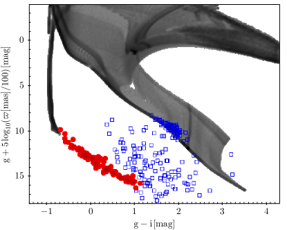
Figure 1: Color-(absolute) magnitude diagram of candidate binary companions to TGAS primary stars (blue). The WDs analyzed in this study are highlighted in red. These candidates were selected to be within $200\,\rm pc$, to have separations $<10,000\,\rm AU$, to have identical joint proper motions within 5$\sigma$. We also eliminated TGAS primaries with very small proper motions to reduce background contamination (see Appendix A). Assuming the candidate secondaries to be equidistant to the TGAS primaries, we can place them on a color-magnitude diagram. The comparison with MESA isochrones (gray dots, Dotter 2016) shows a clear main sequence, and a very clear WD sequence, with some remaining contaminants (that are far from any isochrone or cooling curve). For the present paper, we only consider the candidate WD companions, identified from this diagram (red). (See Appendix A for database query.)

The WD secondaries will generally be much fainter than the MS primaries from TGAS. Therefore, we cannot draw on TGAS for their proper motions. Combining extensive sky coverage ($3\pi$) with proper motion precision and accuracy, the GPS1 catalog (Tian et al., 2017) may be the best current source of such proper motions. Specifically, we queried (see Appendix A) the GPS1 catalog to return the possible companions to all $\sim 100,000$ TGAS stars that had parallax measurements better than $5\%$ and parallax estimates greater than $5\,\rm mas$ (i.e. $<200\,\rm pc$ in the limit of exact parallaxes); we also required that the projected separation corresponded to less than $\leq 10,000\,\rm AU$ and that the proper motions among the potential pair were consistent at the $5\sigma$ level. We further required that the PS1 photometry for the companion was $\sigma<0.05$ mag in $girz$, that the sources had colors consistent with the $(g-r)~{}vs.~{}(r-i)$ color-color locus of WDs. Finally, we eliminated candidates that had very wide separation, yet low proper motions, as they are particularly susceptible to (background) contamination. The specifics are detailed in Appendix A.

This above selection left us with a wide binary sample of about 150 objects, where we expect the companions to the TGAS MS stars to be either fainter MS stars or WDs. Adopting the parallax-distance to the primary MS, we can construct a color – absolute magnitude diagram for the candidate companions, which is shown in Fig.1. It shows both a clear MS and a WD sequence, attesting to the fact that for the most part, we have selected equidistant (and presumably bound) companions; there are few interlopers, apparent in Fig. 1 as objects whose color-magnitude position is inconsistent with stellar isochrones of WD cooling curves. Some of these objects are MS-MS binaries, others may just be background contaminants. For the present paper, we are not interested in the MS secondary components and the obvious interlopers, so we eliminate them from further consideration.

3 Age Constraints on the Wide Binary Systems

We are now left with a set of 91 candidate WDs (cWD), whose distances are precisely constrained by the parallaxes to their companions. Of those, 15 are brighter (Figure 2, red circles) than the predictions from the $0.5\,{\rm M}_{\odot}$ cooling curve of Bergeron et al. (1995), which implies they have masses that are too low to be consistent with single-star evolution during the age of the Universe. Thus, these objects are either the result of common envelope evolution, or are themselves unresolved binary WDs, or the photometry is contaminated, e.g. by a background source. We conservatively eliminate these objects from further consideration in this preliminary work.

To now infer precisely the ages of these WDs, we need to know and compare their trigonometric parallaxes, their spectral energy distributions (SEDs), and their atmospheric types (DA, DB, etc.) to models. Such modeling requires an understanding of WD cooling processes, of the initial-final mass relation (IFMR) of WDs, and an understanding of the precursor stars’ lifetimes as a function of mass and metallicity. In practice, this inference can be accomplished via the software suite BASE-9 (von Hippel et al., 2006; De Gennaro et al., 2008; van Dyk et al., 2009; Stein et al., 2013; Stenning et al., 2016), which fits the SED of each cWD, using the Gaia trigonometric parallax for the MS star as prior information.

For the present context, BASE-9 serves as a flexible software package that combines stellar evolution models (e.g. Dotter et al., 2008), an IFMR (e.g. Salaris et al., 2009; Williams et al., 2009), WD interior cooling models (e.g., Althaus & Benvenuto 1998; Montgomery et al. 1999, updated and expanded for our use in 2011; Renedo et al. 2010), and WD atmosphere models (e.g. Bergeron et al., 1995, updated regularly on-line), with photometric constraints in a wide range of possible passbands. BASE-9 accounts for the individual uncertainties for all data; the ancillary information (e.g. parallax) and astrophysical knowledge are incorporated through the prior distributions. O’Malley et al. (2013) demonstrated BASE-9 derives reliable posterior age distributions for individual field WDs and von Hippel et al (2018, in prep) show how the derived WD age precision depends on WD masses, number and quality of photometric bands, and parallax precision.

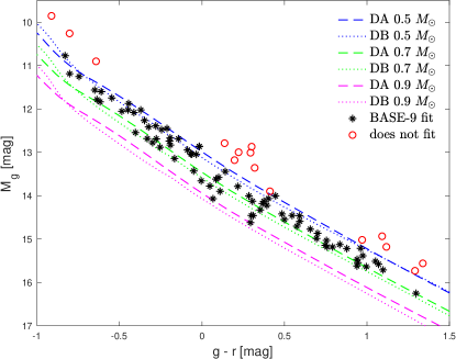
Figure 2: Comparison of the color-(absolute) magnitude distribution of our candidate WDs to a set of cooling curves for DA (dashed; and DB, dotted) WDs with masses between $0.5$ and $0.9\,{\rm M}_{\odot}$. The plot also indicates (red circles) the candidates for which BASE-9 modeling could not find acceptable solutions, presumably because they are not single WDs at the primary star’s distance.

The WD ages we derive below will indicate that these systems are most likely to be disk or thick disk stars. Because we do not yet have spectroscopic abundances (of the MS primary), we set the prior distribution on metallicity to be a broad Gaussian with a mean $\langle\rm[Fe/H]\rangle=-0.5\,\rm dex$ and a dispersion $\sigma(\rm[Fe/H])=1.0\,\rm dex$. While we also do not have the line-of-sight absorption for these stars, they are all closer than $200\,\rm pc$, with most being nearer than $100\,\rm pc$, so we set a strong prior on the absorption of $A_{\rm 0}\approx 0$ mag.

Using these input data and constraints, we ran BASE-9 on each cWD individually, without further knowledge of the properties of its MS companion, employing Dotter et al. (2008) precursor models, the Williams et al. (2009) IFMR, Montgomery et al. (1999) WD interiors, and Bergeron et al. (1995) WD atmospheres. Without spectroscopy, we do not know which objects are H-atmosphere (DA) WDs and which are DBs. Fortunately for our analysis, nature makes predominantly DA WDs ($\sim$75%; Tremblay & Bergeron 2008), and it is therefore a good initial assumption that those cWDs that have posterior distance probabilities consistent with their candidate MS companion Gaia parallaxes, are indeed DAs.

Figure 3 presents the joint posterior distributions (PDF) for eight example WDs. Panels show the zero-age main sequence (ZAMS) mass vs. age plane, with each dot presenting a PDF sample. The panels are sorted in order of increasing mass. The first panel, for WD 1, shows an example where the parallax prior mean is inconsistent with the posterior distance distribution: models would like to predict a star older than the age of the Universe. This star is one of the 15 candidate WDs whose luminosities are above the $0.5\,{\rm M}_{\odot}$ model in Figure 2. For the other seven WDs presented Fig. 3 and for all but the 15 problematical objects identified in Figure 2 (red circles), their posterior distance distributions are consistent with their companion parallax prior, indicating that the model star could readily fit the data at the appropriate luminosity. The age precisions among the eight cases in Figure 2 range from $90\,\rm Myr$ to $1.46\,\rm Gyr$. Four of these eight WDs have fractional age errors of only 3%, and the WD with the poorest age constraint (WD 42, with a ZAMS mass of $1.75\pm 0.15\,{\rm M}_{\odot}$ and age = $2.1\pm 0.5$ $\rm Gyr$) still provides meaningful age information. This figure also indicates that a more constraining parallax prior, which would in turn further constrain the WD mass and thereby its ZAMS mass, would additionally improve the age precision for these WDs.

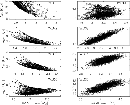
Figure 3: The joint mass vs. age posterior distribution derived from BASE-9 modeling for eight example WD candidates. The panels list the specific WD and are ordered by increase ZAMS mass of the WD. The panels show that there are precise (though covariant) constraints on both the ages and the precursor mass. Note that the first panel presents the case of an overly low inferred WD mass that in practice could not be fit by BASE-9 in a manner consistent with its parallax. The only hint of that issue in this particular diagram is that age is running up against the age of the Universe.

The formal uncertainties in the fitted WD ages are dominated by the parallax precision. While WD models are mature and have benefited from substantial tests in star clusters, nearby binaries, and asteroseismology, the accuracy of the ages may still be poorer than the precision in certain regions of parameter space. Particularly WDs with ZAMS masses $\lesssim 2\,{\rm M}_{\odot}$ or WDs with surface effective temperatures lower than about 5000 K are challenging. Gaia parallaxes tightly constrain the present mass of cool WDs. But when that mass is mapped back onto the ZAMS, small uncertainties in mass transform to large uncertainties in the time a WD spent evolving as a MS star. Additionally, the IFMR is not known perfectly, and small adjustments in the IFMR may change the precursor mass values and thus the pre-WD ages, especially for low-mass precursors. Thus, for those objects, we can derive a precise cooling age, but not a precise total age. For WDs with ${T}_{\rm eff}\leq 5000$ K, issues arise both in our present understanding of their atmospheres and possibly with additional sources of energy release during crystallization (e.g. Horowitz et al., 2010). We can avoid most of these problems by focusing on the WDs in a suitable mass and temperature range. Nevertheless, formal tests on WD ages have not yet been performed at the level of the best of these WD age precisions; we will have to await tests that can be performed in open clusters and WD-WD pairs with Gaia DR2. At this point, we would like to emphasize that the WD ages we derive should be highly precise and deliver excellent relative ages. These ages are likely to be accurate at the 5-10% level, subject to further testing.

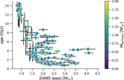
Figure 4: Age in Gyrs vs. ZAMS mass of the precursor in solar units for the 91 WD candidates, all of which are companions to TGAS main sequence stars. Error bars indicate the marginalized $\pm 1\sigma$ age and mass uncertainties; note that in many cases the age uncertainties are smaller than the symbols. Age uncertainties for WDs with precursor ZAMS masses $\leq 1.7\,{\rm M}_{\odot}$ are large, because of the increasing fraction of the system lifetime spent on the MS (rather than as a cooling WD). The color indicates the mass of the MS primary, showing that most of them are low-mass stars ($M\lesssim 1\,{\rm M}_{\odot}$), whose ages could not be inferred well from isochrones or asteroseismology.

The 91 WDs that BASE-9 fit consistently with the parallaxes are plotted in Figure 4. The error bars represent $\pm$1 standard deviations in age and ZAMS mass, respectively. Their colors indicate the approximative initial mass of their MS companion using their 2MASS photometry (and the strong prior that they live on the main-sequence). Age uncertainties drop rapidly with ZAMS masses $\geq 1.7\,{\rm M}_{\odot}$. The relative age uncertainties, in the sense $\sigma(\tau_{age})/\langle\tau_{age}\rangle$, range from the highly precise value of 1.9% to as poor as 54.5% at the low ZAMS mass end. Of these 91 WDs, 42 have relative age precisions better than 10% and 67 have relative age precisions of better than 20%. The objects plotted in Figure 4 are both the largest sample of field WDs and the largest sample of WD - MS pairs with precise ages.

4 Discussion and Outlook

In this paper we carried out a pilot study for one of the many applications of using Gaia data to constrain stellar properties. We identified systems where Gaia parallaxes gave us distances to nearby ($<200\,\rm pc$) main sequence stars, and where common proper motion information from the GPS1 catalog provided strong evidence for a wide (and equidistant) WD companion. Our analysis nearly doubles the number of such known wide binaries with parallax distances.

We applied the BASE-9 modeling to infer ages for the white dwarfs, which must be the same as those of the MS stars. Achieving better than 10% age precision for 42 systems, and better than 20% for another 25 systems (67 in total) constitutes an order of magnitude increase in the number of low-mass ($\sim 1~{}N_{\odot}$) MS field stars for which ages are known with that precision. This approach seems particularly suited to obtain precise ages for low-mass ($<1\,{\rm M}_{\odot}$) MS stars, where most other methods fail for field stars. The majority of our systems have ages of 1-8 $\rm Gyr$, an age range that is poorly sampled by known clusters.

To realize the scientific potential of the sample at hand, spectroscopic follow-up is necessary in two respects. First, simple low-resolution spectroscopy needs to verify which of these WDs are actually DA WD’s, as assumed in the modeling. Second, higher-resolution spectroscopy of the bright ($m<11$ mag) MS stars should be used to determine their detailed abundance pattern, to increase well-calibrated constraints of $[\vec{X}/Fe]$, i.e., $\tau_{age}$ for chemical evolution modeling. We are currently pursuing this follow-up.

While this particular sample will of course be superseded by the data from Gaia’s DR2 (in April 2018), this overall approach will be particularly powerful in light of the full Gaia data. For studying the WD’s themselves, precise parallaxes will be paramount, especially for the oldest and faintest WDs. In these case, the boost in parallax precision transferred from the MS star, will aid the analysis. In turn, identifying WD companions to MS stars mostly by their common proper motion, will greatly enlarge the volumes over which this analysis can be done (compared to insisting on precise parallaxes for both the MS and the WD).

Appendix A GPS1$\times$TGAS Query

In this section, we detail the selection query we performed on TGAS and GPS1 catalogs.

Matching GPS1 against TGAS will report all the stars from GPS1 within some radius that could potentially be associated with a TGAS bright star. If we also filter on parallax and motion similarity this will only give co-moving pairs. We consider nearby objects according to TGAS parallaxes as

$$\begin{split}\textrm{distance}((\alpha,\delta)_{GPS1},&(\alpha,\delta)_{TGAS})\,[\rm deg]\\ &<10.3\times\frac{\varpi[\rm mas]}{3600}.\end{split}$$ (A1)

Further tuning can be done by adding a contamination model, though this is out of the proof-of-concept scope of this paper. In addition, we need to only conserve good parallaxes within a $200\,\rm pc$ ($5\,\rm mas$) volume around the Sun as

$$\begin{split}&\varpi\geq 5\,\rm mas\\ &\frac{\varpi}{\sigma_{\varpi}}>20,\end{split}$$ (A2)

and relatively good motion precision in GPS1

$$\sqrt{\sigma^{2}_{\mu,\alpha}+\sigma^{2}_{\mu,\delta}}<6\,\rm mas.yr^{-1}$$ (A3)

Additionally, we want pairs of objects that are co-moving according to both surveys (within their uncertainties). Therefore we select pairs that appear co-moving within $5-\sigma$ uncertainties:

$$\begin{split}&\frac{\left((\mu_{\alpha}^{\star})_{GPS1}-(\mu_{\alpha}^{\star})_{TGAS}\right)^{2}}{\left((\sigma_{\mu,\alpha})_{GPS1}^{2}+(\sigma_{\mu,\alpha})_{TGAS}^{2}\right)}\\ \quad&+\frac{\left((\mu_{\delta})_{GPS1}-(\mu_{\delta})_{TGAS}\right)^{2}}{\left((\sigma_{\mu,\delta})_{GPS1}^{2}+(\sigma_{\mu,\delta})_{TGAS}^{2}\right)}\leq(5\,\rm mas.yr^{-1})^{2}.\end{split}$$ (A4)

However, many objects with small motion where actually contaminant or main-sequence objects. Therefore we also include a revised cut that rejects objects with small motions (despite leading to incompleteness):

$$\begin{split}&\sqrt{(\mu_{\alpha}^{\star})_{TGAS}^{2}+(\mu_{\delta})_{TGAS}^{2}}~{}[\rm mas.yr^{-1}]\\ \quad&>{25}\left(\frac{1000}{0.3\,\varpi[\rm mas]}\times\textrm{distance}((\alpha,\delta)_{GPS1},(\alpha,\delta)_{TGAS})\right)^{0.7}.\end{split}$$ (A5)

Note that the constant and power of the above equation are results of an empirical inspection. Finally, we also added color terms that avoid having main-sequence objects and we also select good photometry for their SED analysis. Based on empirical definitions we added the following selections:

$$\begin{split}&\left|(g-i)-1.6\times(g-r)+0.1\right|<0.15\,\mathrm{mag},\\ &\left(\sigma_{g},\,\sigma_{r},\,\sigma_{i},\,\sigma_{z}\right)<0.05\,\mathrm{mag},\end{split}$$ (A6)

This selection translates into the following ADQL query. As GAVO is currently the only service providing the GPS1 catalog, the field names correspond to their definition, and may vary when using other sources (e.g., VizieR, Gaia Archive).

SELECT
    db.obj_id, db.ra, db.dec, db.e_ra, db.e_dec, db.pmra, db.e_pmra,
    db.pmde, db.e_pmde, db.magg,  db.e_magg, db.magr,  db.e_magr,
    db.magi, db.e_magi, db.magz, db.e_magz, db.magy, db.e_magy,
    db.magj, db.e_magj, db.magh, db.e_magh, db.magk, db.e_magk,
    db.maggaia, db.e_maggaia,  tc.source_id, tc.ra, tc.dec,
    tc.ra_error, tc.dec_error, tc.l, tc.b, tc.pmra, tc.pmdec,
    tc.pmra_error, tc.pmdec_error, tc.parallax, tc.parallax_error,
    tc.phot_g_mean_mag,  tc.phot_variable_flag,
    tc.astrometric_excess_noise_sig, tc.ra_dec_corr, tc.ra_pmra_corr,
    tc.ra_pmdec_corr, tc.dec_pmra_corr, tc.dec_pmdec_corr,
    tc.pmra_pmdec_corr, tc.ra_parallax_corr, tc.dec_parallax_corr,
    tc.parallax_pmra_corr, tc.parallax_pmdec_corr, tc.phot_g_n_obs,
    distance(POINT(icrs, db.ra, db.dec),
             POINT(icrs, tc.ra, tc.dec)) AS pairdistance
FROM tgas.main AS tc
JOIN gps1.main AS db
ON
    1 = contains(POINT(ICRS, db.ra, db.dec),
                 CIRCLE(ICRS, tc.ra, tc.dec, 10.3 * tc.parallax/3600.))
WHERE
    parallax >= 5 AND parallax / parallax_error > 20
AND
    (power((db.pmra * 3.6 * 1e6 - tc.pmra), 2) /
        (power(db.e_pmra * 3.6 * 1e6 ,2) + power(tc.pmra_error, 2))  +
        power((db.pmde * 3.6 * 1e6 - tc.pmdec), 2) /
            (power(db.e_pmde * 3.6 * 1e6,2) + power(tc.pmdec_error, 2))
     ) < 25
AND
    sqrt((power(tc.pmra, 2)+ power(tc.pmdec, 2) )) >
      25 *  power(distance(POINT(’icrs’, db.ra, db.dec),
                           POINT(’icrs’, tc.ra, tc.dec))
                  * (100./tc.parallax) / 0.03, 0.7)
AND
    db.e_magg < 0.05 AND  db.e_magr < 0.05
AND
    db.e_magi < 0.05 AND db.e_magz < 0.05
AND
    abs((magg - magi) - 1.6*(magg - magr)+0.1) < 0.15

Note that on Fig.1, the red selection corresponds to this query, while the blue selection results from the same query were we only apply the JOIN and the two first WHERE conditions.

Appendix B Catalogs

In this section we describe the content of the catalog generated during this study.

The catalog contains the photometric and astrometric data for all of the WD candidates of this study. For each star, we also provide the mean, median and standard deviation of the posterior PDF of the WD properties, esp. age and ZAMS mass. In addition, the catalog contains the matched MS component 2MASS (J, H, K), and WISE (W1, W2, W3, W4) photometry as well as our mass estimates and uncertainties.

Table 1: Catalog column description

Column	Units	Description	Column	Units	Description
source_id		Gaia DR1 identifier	AllWISE		AllWise identifier
magg	mag	Gaia DR1 $G$ magnitude (of the WD)	gps1_ra	deg	right ascension from GPS1
e_magg	mag	Gaia $G$ magnitude uncertainty	gps1_dec	deg	declination from GPS1
magr	mag	GPS1 $r$ magnitude	gps1_e_ra	deg	GPS1 RA uncertainty
e_magr	mag	GPS1 $r$ uncertainty	gps1_e_dec	deg	GPS1 DEC uncertainty
magi	mag	GPS1 $i$ magnitude	gps1_pmra	deg/yr-1	GPS1 $\mu_{\alpha}^{\star}$
e_magi	mag	GPS1 $i$ uncertainty	gps1_pmde	deg/yr-1	GPS1 $\mu_{\delta}$
magz	mag	GPS1 $z$ magnitude	gps1_e_pmde	deg/yr-1	GPS1 $\mu_{\alpha}^{\star}$ uncertainty
e_magz	mag	GPS1 $z$ uncertainty	gps1_e_pmra	deg/yr-1	GPS1 $\mu_{\delta}$ uncertainty
magy	mag	GPS1 $y$ magnitude	primary_Hmag	mag	primary $H$ photometry
e_magy	mag	GPS1 $y$ uncertainty	primary_Jmag	mag	primary $J$ photometry
magj	mag	GPS1 $J$ magnitude	primary_Kmag	mag	primary $K$ photometry
e_magj	mag	GPS1 $J$ uncertainty	primary_W1mag	mag	primary $W1$ photometry
magh	mag	GPS1 $H$ magnitude	primary_W2mag	mag	primary $W2$ photometry
e_magh	mag	GPS1 $H$ uncertainty	primary_W3mag	mag	primary $W3$ photometry
magk	mag	GPS1 $K$ magnitude	primary_W4mag	mag	primary $W4$ photometry
e_magk	mag	GPS1 $K$ uncertainty	primary_e_Hmag	mag	primary $H$ uncertainty
maggaia	mag	GPS1 Gaia $G$ magnitude	primary_e_Jmag	mag	primary $J$ uncertainty
e_maggaia	mag	GPS1 converted Gaia $G$ uncertainty	primary_e_Kmag	mag	primary $K$ uncertainty
parallax	$\rm mas$	Gaia DR1 Parallax (Primary)	primary_e_W1mag	mag	primary $W1$ uncertainty
parallax_error	$\rm mas$	Gaia DR1 parallax uncertainty	primary_e_W2mag	mag	primary $W2$ uncertainty
mn_Age	$\rm Gyr$	posterior mean WD age	primary_e_W3mag	mag	primary $W3$ uncertainty
mn_fe	dex	posterior mean $\rm[Fe/H]$	primary_e_W4mag	mag	primary $W4$ uncertainty
mn_mod	mag	posterior mean distance modulus	primary_mass_p16	${\rm M}_{\odot}$	16th mass percentile
mn_mass	${\rm M}_{\odot}$	posterior mean WD mass	primary_mass_p50	${\rm M}_{\odot}$	50th mass percentile
mn_cAge	$\rm Gyr$	posterior mean WD cooling age	primary_mass_p84	${\rm M}_{\odot}$	84th mass percentile
mn_pAge	$\rm Gyr$	posterior mean WD precusor’s age	tgas_ra	deg	right ascension from TGAS
md_Age	$\rm Gyr$	posterior median WD age	tgas_ra_error	$\rm mas$	TGAS right ascension uncertainty
md_fe	dex	posterior median $\rm[Fe/H]$	tgas_dec	deg	declination from TGAS
md_mod	mag	posterior median distance modulus	tgas_dec_error	$\rm mas$	TGAS declination uncertainty
md_mass	${\rm M}_{\odot}$	posterior median WD mass	tgas_b	deg	Galactic latitude from TGAS
md_cAge	$\rm Gyr$	posterior median WD cooling age	tgas_l	deg	Galactic longitude from TGAS
md_pAge	$\rm Gyr$	posterior median WD precusor’s age	tgas_Gmag	mag	primary TGAS G magnitude
st_Age	$\rm Gyr$	posterior standard deviation WD age	tgas_pmdec	$\rm mas.yr^{-1}$	TGAS $\mu_{\alpha}^{\star}$
st_fe	dex	posterior standard deviation $\rm[Fe/H]$	tgas_pmdec_error	$\rm mas.yr^{-1}$	TGAS $\mu_{\alpha}^{\star}$ uncertainty
st_mod	mag	posterior standard deviation distance modulus	tgas_pmra	$\rm mas.yr^{-1}$	TGAS $\mu_{\delta}$
st_mass	${\rm M}_{\odot}$	posterior standard deviation WD mass	tgas_pmra_error	$\rm mas.yr^{-1}$	TGAS $\mu_{\delta}$ uncertainty
st_cAge	$\rm Gyr$	posterior standard deviation WD cooling age	primary_source_id		primary TGAS DR1 identifier
st_pAge	$\rm Gyr$	posterior standard deviation WD precusor’s age

References

- Althaus & Benvenuto (1998) Althaus, L. G., & Benvenuto, O. G. 1998, MNRAS, 296, 206
- Angus et al. (2015) Angus, R., Aigrain, S., Foreman-Mackey, D., & McQuillan, A. 2015, MNRAS, 450, 1787
- Bergeron et al. (2001) Bergeron, P., Leggett, S. K., & Ruiz, M. T. 2001, ApJS, 133, 413
- Bergeron et al. (1995) Bergeron, P., Wesemael, F., & Beauchamp, A. 1995, PASP, 107, 1047
- Chaplin et al. (2014) Chaplin, W. J., Basu, S., Huber, D., Serenelli, A., Casagrande, L., Silva Aguirre, V., Ball, W. H., Creevey, O. L., Gizon, L., Handberg, R., Karoff, C., Lutz, R., Marques, J. P., Miglio, A., Stello, D., Suran, M. D., Pricopi, D., Metcalfe, T. S., Monteiro, M. J. P. F. G., Molenda-Żakowicz, J., Appourchaux, T., Christensen-Dalsgaard, J., Elsworth, Y., García, R. A., Houdek, G., Kjeldsen, H., Bonanno, A., Campante, T. L., Corsaro, E., Gaulme, P., Hekker, S., Mathur, S., Mosser, B., Régulo, C., & Salabert, D. 2014, ApJS, 210, 1
- De Gennaro et al. (2008) De Gennaro, S., von Hippel, T., Winget, D. E., Kepler, S. O., Nitta, A., Koester, D., & Althaus, L. 2008, AJ, 135, 1
- Dotter (2016) Dotter, A. 2016, ApJS, 222, 8
- Dotter et al. (2008) Dotter, A., Chaboyer, B., Jevremović, D., Kostov, V., Baron, E., & Ferguson, J. W. 2008, ApJS, 178, 89
- Gaia Collaboration et al. (2016) Gaia Collaboration, Brown, A. G. A., Vallenari, A., Prusti, T., de Bruijne, J. H. J., Mignard, F., Drimmel, R., Babusiaux, C., Bailer-Jones, C. A. L., Bastian, U., & et al. 2016, A&A, 595, A2
- Horowitz et al. (2010) Horowitz, C. J., Schneider, A. S., & Berry, D. K. 2010, Physical Review Letters, 104, 231101
- Montgomery et al. (1999) Montgomery, M. H., Klumpe, E. W., Winget, D. E., & Wood, M. A. 1999, ApJ, 525, 482
- O’Malley et al. (2013) O’Malley, E. M., von Hippel, T., & van Dyk, D. A. 2013, ApJ, 775, 1
- Renedo et al. (2010) Renedo, I., Althaus, L. G., Miller Bertolami, M. M., Romero, A. D., Córsico, A. H., Rohrmann, R. D., & García-Berro, E. 2010, ApJ, 717, 183
- Salaris et al. (2009) Salaris, M., Serenelli, A., Weiss, A., & Miller Bertolami, M. 2009, ApJ, 692, 1013
- Soderblom (2010) Soderblom, D. R. 2010, ARA&A, 48, 581
- Stein et al. (2013) Stein, N. M., van Dyk, D. A., von Hippel, T., DeGennaro, S., Jeffery, E. J., & Jefferys, W. H. 2013, Statistical Analysis and Data Mining: The ASA Data Science Journal, Vol. 9, Issue 1, p. 34-52, 6, 34
- Stenning et al. (2016) Stenning, D. C., Wagner-Kaiser, R., Robinson, E., van Dyk, D. A., von Hippel, T., Sarajedini, A., & Stein, N. 2016, ApJ, 826, 41
- Tian et al. (2017) Tian, H.-J., Gupta, P., Sesar, B., Rix, H.-W., Martin, N. F., Liu, C., Goldman, B., Platais, I., Kudritzki, R.-P., & Waters, C. Z. 2017, ApJS, 232, 4
- Torres et al. (2010) Torres, G., Andersen, J., & Giménez, A. 2010, A&A Rev., 18, 67
- Tremblay & Bergeron (2008) Tremblay, P.-E., & Bergeron, P. 2008, ApJ, 672, 1144
- Tremblay et al. (2017) Tremblay, P.-E., Gentile-Fusillo, N., Raddi, R., Jordan, S., Besson, C., Gänsicke, B. T., Parsons, S. G., Koester, D., Marsh, T., Bohlin, R., Kalirai, J., & Deustua, S. 2017, MNRAS, 465, 2849
- van Dyk et al. (2009) van Dyk, D. A., Degennaro, S., Stein, N., Jefferys, W. H., & von Hippel, T. 2009, Annals of Applied Statistics, 3, 117
- von Hippel et al. (2006) von Hippel, T., Jefferys, W. H., Scott, J., Stein, N., Winget, D. E., De Gennaro, S., Dam, A., & Jeffery, E. 2006, ApJ, 645, 1436
- Williams et al. (2009) Williams, K. A., Bolte, M., & Koester, D. 2009, ApJ, 693, 355