DESY 18-022 KIAS-P18014 WU-HEP-18-03 Seesaw mechanism in magnetic compactifications

1 Introduction

The standard model (SM) of elementary particles has been completed by the discovery of the last puzzle piece, i.e., the Higgs boson in 2012 [1, 2]. Before discovering the Higgs boson, the non-vanishing neutrino masses reported in 1996 have demanded that the SM must be extended to its neutrino sector with right-handed neutrinos. Recently, the neutrino flavor structures have been steadily revealed from the viewpoints of neutrino oscillations [3, 4] and cosmological behaviors of neutrinos [5]. The precise theoretical investigation in the neutrino flavor structure can be one of the main pillars in the modern particle physics.

In contrast to the other SM three-generation fermions, i.e., quarks and charged leptons, several experiments have shown that the neutrinos have tiny masses around eV scale. This experimental result implicitly tells that there may be a particular mechanism only in the neutrino sector. One of the mechanisms which can explain the tiny neutrino masses is the (type I) seesaw mechanism [6, 7, 8, 9, 10] by means of the right-handed neutrino Majorana mass term. Only by adding the heavy Majorana mass term at some high scale in addition to the Dirac mass term, the effective neutrino masses can be small enough for the experimental results, even if the Dirac mass term appears around the electroweak (EW) scale. Although the seesaw mechanism is quite simple and beneficial in many scenarios, there is still an ambiguous point in the detailed structures of the Dirac and Majorana mass matrices. In usual bottom-up approaches where one assumes some extensions to the SM, it is generically difficult to theoretically determine the concrete entries and values in the mass matrices. Then, in order to control the matrix entries, one pursuits the models with the continuous flavor symmetry [11], the discrete flavor symmetry [12] and the extra dimension(s) [13], for instance.

As well as the matrix entries in the neutrino sector, to understand an origin of the three-generation structure behind the SM fermions is still a challenging issue. Among recent topics, an interesting attempt to reveal the generation structure is to add magnetic fluxes on compactified extra dimensions. In particular, the magnetic fluxes turned on the torus provide multiple massless wavefunctions after the Kaluza–Klein (KK) decomposition of fields [14, 15]. The same happens in the extensions to toroidal orbifolds [16, 17, 18] in particular those with discrete Wilson line phases [19, 20, 21, 22, 23]. Since such multiple massless modes belong to the same representation of fields, the multiplicity of massless modes should be identified as the generation structure in the SM. Many model constructions by means of the mechanism have been done especially in the past five years, for example, supersymmetric models [24, 25], non-supersymmetric models [26], systematic searches of three-generation models [27, 28, 29], three-generation models with broken supersymmetry [30], quark and charged lepton mass matrices from bulk overlap integrals [26, 25] and brane-localized Yukawa couplings [30, 31, 32], mass spectra in the presence of brane-localized mass terms [33] and cosmological inflation model [34], applications to volume moduli stabilization [35, 36].

It is noted that we face difficulties in generating the neutrino Majorana mass term in the previous model buildings based on extra dimensional fluxes [24]. In this paper, the brane-localized mass term(s) on a toroidal orbifold $T^{2}/Z_{2}$ analyzed in [33] is applied to the type I seesaw scenario. Then, the Majorana mass matrix is analytically given by the localized neutrino masses and concrete values are determined by the values of zero-mode wavefunctions evaluated at orbifold fixed points. In addition, the Dirac mass matrix originates from the Yukawa couplings which are analytically calculated by overlap integrals of zero-mode wavefunctions. Thus, the seesaw mechanism in terms of brane-localized neutrino masses at fixed points of $T^{2}/Z_{2}$ with extra dimensional fluxes is a simple and typical scenario.

This paper is organized as follows. In Sec. 2, we briefly review several ingredients for the seesaw mechanism in the orbifold $T^{2}/Z_{2}$ on flux background. In Sec. 3, five patterns of neutrino mass matrices realized on such an orbifold are numerically analyzed and compared with observed values by recent neutrino oscillation experiments. We make conclusion in Sec.  4.

2 Review of $T^{2}/Z_{2}$ orbifold with fluxes

In this section, we briefly review the six-dimensional (6D) compactification on the orbifold $T^{2}/Z_{2}$ with fluxes, and show the KK mass spectra and wavefunctions as well as (three-point) Yukawa coupling constants. In seesaw scenarios, such Yukawa couplings between neutrinos and the Higgs boson provide the Dirac mass matrix after the Higgs boson develops its vacuum expectation value (VEV). On another hand, the Majorana mass term for the seesaw originates from the existence of brane-localized term(s) at orbifold fixed points of $T^{2}/Z_{2}$. This section is mainly based on [33, 15, 17, 41].

2.1 Flux background and Yukawa couplings

We consider the 6D gauge theory compactified on $\mathcal{M}^{4}\times T^{2}/Z_{2}$. Here, $\mathcal{M}^{4}$ is the four-dimensional (4D) Minkowski spacetime and we choose $T^{2}/Z_{2}$ to be extra dimensions of our model.

We first start in a two-dimensional torus $T^{2}$. We define two oblique coordinates $y_{5}$ and $y_{6}$ as coordinates of $T^{2}$ and such coordinates are often conveniently expressed by the complex coordinate $z=(y_{5}+\tau y_{6})/(2\pi R)$, with a complex structure modulus $\tau\in\mathbb{C}\,\,{({\rm Im}\,\tau>0)}$ and a radius $R$, where a schematic picture is depicted in Fig. 1. Notice that the radius $R$ is associated with a compactification scale $M_{C}\sim 1/R$. The toroidal orbifold $T^{2}/Z_{2}$ is obtained by the identifications in the two-dimensional extra dimensions under the toroidal periodicities and the $Z_{2}$ rotation,

$$z\sim z+1\sim z+\tau\sim-z.$$ (1)

In accordance with the above identifications, there appear four fixed points on $T^{2}/Z_{2}$, i.e., at $z=$ $0,1/2,\tau/2$ and $(1+\tau)/2$, as described in Fig. 1.

Kinetic terms of 6D Weyl fermions and scalars are given as

$$\mathcal{L}_{\rm kin}=\int d^{4}x\int_{T^{2}}d^{2}z\,{\left\{i\bar{\Psi}\Gamma^{M}D_{M}\Psi+(D_{M}\Phi)^{\dagger}(D^{M}\Phi)\right\}}.$$ (2)

In Eq. (2), $M$ runs over $0,1,2,3,5,6$, $\Gamma^{M}$ denotes the gamma matrices describing the Clifford algebra in six dimensions, and $D_{M}=\partial_{M}-iqA_{M}$ denotes a covariant derivative under a $U(1)$ gauge symmetry. In the following, we discuss the toroidal case at the first step and, then extend it to the toroidal orbifold case. In the six-dimensional action, we assume that the vector potential $A_{m}\,\,(m=5,6)$ possesses classical non-trivial background $b=\int_{T^{2}}F$ of the field strength $F=(ib/2{\rm Im}\tau)dz\wedge d\bar{z}$:

$$A^{(b)}(z)=\frac{b}{2{\rm Im}\,\tau}{\rm Im}\,(\bar{z}dz).$$ (3)

The consistency condition provides the quantization condition of fluxes:

$$\frac{qb}{2\pi}=M\in\mathbb{Z}.$$ (4)

It should be mentioned that there is a controversial point about the Dirac charge quantization condition (4). As naturally expected, several papers [14, 16, 21] claim that a flux density of bulk constant flux is twice as that on the original torus. On the other hand, some of research groups [17, 19] have investigated it in the framework of conformal field theory and have reported different quantization conditions, i.e., the same one as the original torus. One of their claims is that Eq. (3) behaves as an appropriate $U(1)$ connection on the orbifold even with the original charge quantization (4). Throughout this paper, we follow the latter condition.

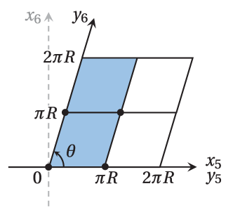
Figure 1: The fundamental domain of the orbifold $T^{2}/Z_{2}$ is shown. The shaded region is a fundamental region and the black dots represent the four fixed points of the orbifold. This figure is drawn for a generic complex structure $\tau\in\mathbb{C}$, where an angle between $y_{5}$ and $y_{6}$ is given as $\cos\theta\equiv{\rm Re}\,\tau/|\tau|$.

We perform the KK decomposition of six-dimensional fields. The six-dimensional Weyl fermions and scalars are decomposed as

$$\Psi(x^{\mu},z)=\sum_{n}\chi_{n}(x^{\mu})\otimes\psi_{n}(z),$$ (5)

$$\Phi(x^{\mu},z)=\sum_{n}\varphi_{n}(x^{\mu})\otimes\phi_{n}(z).$$ (6)

The fermion wave functions in the extra two directions are determined as eigenstates of the Dirac operator in extra dimensional directions,

$$i\Gamma^{m}D_{m}\psi_{n}(z)=m_{n}\psi_{n}(z),$$ (7)

where $m=5,6$ and $m_{n}\ (n=0,1,2\cdots)$ denote the KK mass spectrum. Hence, zero-mode equations for $n=0$ ($m_{0}=0$) are given in terms of $D\equiv D_{5}+\tau D_{6}$ as

$$D\,\psi_{+}(z)=0,\ \qquad D^{\dagger}\,\psi_{-}(z)=0,$$ (8)

where the two-dimensional spinor is decomposed into $\psi_{0}=\left(\psi_{+},\psi_{-}\right)^{T}$ with the two-dimensional internal chiralities. In several appropriate boundary conditions associated with necessary gauge transformations, we describe zero-mode wave functions analytically in terms of the Jacobi theta function [15],

$$\psi_{+}^{j}(z) \equiv\Theta^{j,M}(z)$$

$$={\mathcal{N}_{M}}\,e^{i\pi Mz{\rm Im}\,z/{\rm Im}\,\tau}\cdot\vartheta\begin{bmatrix}j/M\\[5.0pt] 0\end{bmatrix}\left(Mz,M\tau\right)\qquad(j=0,1,2,\cdots,M-1),$$ (9)

for $M>0$. Here, ${{\cal N}_{M}}=(2M/{\cal A}^{2})^{1/4}$ is a normalization constant [15], where $\mathcal{A}$ represents the area of the torus and ${\cal N}_{M}$ has mass dimension $+1$. If the flux number $M$ is positive (negative), there is no normalizable solution in $\psi_{-}$ ($\psi_{+}$). Notice that Eq. (9) tells that Eq. (8) has $|M|$-independent solutions. Hence we can identify this degeneracy of zero-modes with a family structure for particles in the four-dimensional effective theory. Therefore, if we introduce a non-zero magnetic flux, a chiral structure of the Weyl spinor appears in the four-dimensional effective theory. The form of the KK masses is obtained as

$$m_{n}^{2}=\frac{4\pi M}{\cal A}n.$$ (10)

Also, we similarly compute a scalar wave function as the same as the fermionic one in Eq. (9). There is no massless (zero-)mode in the scalar field. In other words, the lowest KK mass is non-vanishing, where the KK mass spectrum for scalars is given as

$$m_{n}^{2}=\frac{4\pi M}{\cal A}\left(n+\frac{1}{2}\right).$$ (11)

Next, we move to $Z_{2}$ eigenstates of zero-modes under the twisted $Z_{2}$ projection, i.e., $z\sim-z$. The eigenstates of zero-modes on $T^{2}/Z_{2}$ are expressed as linear combinations of those in $T^{2}$ shown in Eq. (9) [16, 17],

$$\Theta^{j,M}_{T^{2}/Z_{2},\eta}(z) = \frac{1}{\sqrt{2}}\left(\Theta^{j,M}(z)+\eta\Theta^{j,M}(-z)\right)$$ (12)

$$= \frac{1}{\sqrt{2}}\left(\Theta^{j,M}(z)+\eta\Theta^{M-j,M}(z)\right),$$

where $\eta$ denotes a $Z_{2}$ parity so as to be the $Z_{2}$ even (odd) as $\eta=+1\ (-1)$. As calculated in [17, 19], the relation between flux numbers and the numbers of zero-mode wave functions are obtained as Tab. 1.

$M$	$0$	$1$	$2$	$3$	$4$	$5$	$6$	$7$	$8$	$\cdots$	$2k$	$2k+1$
$\eta=+1$	$1$	$1$	$2$	$2$	$3$	$3$	$4$	$4$	$5$	$\cdots$	$k+1$	$k+1$
$\eta=-1$	$0$	$0$	$0$	$1$	$1$	$2$	$2$	$3$	$3$	$\cdots$	$k-1$	$k$

Table 1: The relation between flux numbers and the numbers of zero-mode wave functions.

Using the above analytic form of zero-mode eigenstates on $T^{2}/Z_{2}$, we can also analytically calculate Yukawa couplings as an overlap integral of three zero-modes. First, we show the form of Yukawa couplings on $T^{2}$, and then extend them to those of $T^{2}/Z_{2}$. Among only zero-modes, effective Yukawa couplings after dimensional reduction can be computed from the six-dimensional Lagrangian,

$$\mathcal{L}_{\rm Yukawa} = \int_{T^{2}}d^{2}z\left\{-g\overline{\Psi_{1}}\Psi_{2}\Phi+{\rm h.c.}\right\}$$ (13)

$${\supset} -\left(g\int_{T^{2}}d^{2}z\,\Theta^{i,M_{1}}(z)\Theta^{j,M_{2}}(z)\bigl{(}\Theta^{k,M_{3}}(z)\bigr{)}^{*}\right)\overline{\chi_{1}^{{i}}}{\chi_{2}^{{j}}}\varphi^{k}+{\rm h.c.},$$

where we suppose $|M_{3}|\geq|M_{1}|,|M_{2}|$. It is noted that the coefficient $g$ has mass dimension $-1$. Hence, Yukawa couplings can be expressed as

$$Y^{ijk}=g\int_{T^{2}}d^{2}z\,\Theta^{i,M_{1}}(z)\Theta^{j,M_{2}}(z)\bigl{(}\Theta^{k,M_{3}}(z)\bigr{)}^{*}.$$ (14)

As calculated in [15], it is straightforward to perform an integration in Yukawa couplings and we finally obtain

$$Y^{ijk}=g\,{\frac{\mathcal{N}_{|M_{1}|}\mathcal{N}_{|M_{2}|}}{\mathcal{N}_{|M_{3}|}}}\,\sum_{m=0}^{|M_{3}|-1}\vartheta\begin{bmatrix}\frac{M_{2}i-M_{1}j+M_{1}M_{2}m}{M_{1}M_{2}M_{3}}\\[5.0pt] 0\end{bmatrix}(0,\tau M_{1}M_{2}M_{3})\times\delta_{i+j+M_{1}m,k+M_{3}l},$$ (15)

where the overall coupling is a dimensionless factor.

Now, we extend this formula of Yukawa couplings to those of $T^{2}/Z_{2}$. In this case, Yukawa couplings can be expressed as

$$Y^{ijk}_{T^{2}/Z_{2}}=g\int_{T^{2}}d^{2}z\,\Theta^{i,M_{1}}_{T^{2}/Z_{2},\eta_{1}}(z)\Theta^{i,M_{2}}_{T^{2}/Z_{2},\eta_{2}}(z)\bigl{(}\Theta^{i,M_{3}}_{T^{2}/Z_{2},\eta_{3}}(z)\bigr{)}^{*}.$$ (16)

Using Eqs. (12) and (14), Yukawa couplings on $T^{2}/Z_{2}$ are described as

$$Y^{ijk}_{T^{2}/Z_{2}} = \frac{1}{2\sqrt{2}}\left(Y^{ijk}+\eta_{1}Y^{(M_{1}-i)jk}+\eta_{2}Y^{i(M_{2}-j)k}+\eta_{3}Y^{ij(M_{3}-k)}\right.$$ (17)

$$\ \ \ \ \ \ \ \ +\eta_{1}\eta_{2}Y^{(M_{1}-i)(M_{2}-j)k}+\eta_{2}\eta_{3}Y^{i(M_{2}-j)(M_{3}-k)}+\eta_{1}\eta_{3}Y^{(M_{1}-i)j(M_{3}-k)}$$

$$\ \ \ \ \ \ \ \ \left.+\eta_{1}\eta_{2}\eta_{3}Y^{(M_{1}-i)(M_{2}-j)(M_{3}-k)}\right).$$

The concrete entries in Yukawa couplings are analytically written in the appendices of [28, 41] for arbitrary configurations of fluxes and (discrete) Wilson lines. A selection rule is found that Yukawa interaction terms in the Lagrangian must be invariant under the $Z_{2}$ parity transformation. Thus, we have to only consider the four patterns for $\eta_{1},\eta_{2},{\rm and}\ \eta_{3}$ as $(\eta_{1},\eta_{2},\eta_{3})=(+1,+1,+1),\,(+1,-1,-1),\,(-1,+1,-1),\,(-1,-1,+1)$.

2.2 Brane-localized Majorana mass terms

In this paper, we focus on the Majorana mass terms localized at the orbifold fixed points in [33],

$$\mathcal{L}_{\rm brane}=-{\frac{1}{2}}\int_{{T^{2}}}d^{2}z\,\sum_{k=1}^{4}h_{k}\overline{(\Psi_{R})^{C}}\Psi_{R}\,\delta^{2}(z-z_{k})+\text{h.c.},$$ (18)

where $h_{k}\,\,(k=1,2,3,4)$ are constants with mass dimension $-1$. Here, we assume that only the component with the 4D right-hand chirality $(R\,)$ of the 6D Weyl spinor $\Psi$ contributes to the terms. In addition, the 4D Weyl field $\Psi_{R}$ carries a $U(1)$ charge (or flux). Unless the $U(1)$ symmetry generating family structures is broken, the above localized Majorana mass term cannot be written down. Constructing a concrete model by introducing a scalar field for spontaneous breaking of the $U(1)$ (or embedding our setup into more fundamental theories) is beyond the interest of our paper on the observed neutrino profiles. For the moment, we assume an appropriate $U(1)$ breaking mechanism. In the final section, we will comment on how to treat the $U(1)$ symmetry in details. The superscript $C$ denotes the 4D charge conjugation and $z_{k}\,\,(k=1,2,3,4)$ denote the $Z_{2}$ fixed points, i.e.,

$$z_{1}=0,\qquad z_{2}=1/2,\qquad z_{3}=\tau/2,\qquad z_{4}=(1+\tau)/2{.}$$ (19)

The effective Majorana mass matrix in the low energy effective Lagrangian can be computed as

$$\mathcal{L}_{\rm brane} = -{\frac{1}{2}}\sum_{k=1}^{4}h_{k}\left(\int_{{T^{2}}}d^{2}z\,\Theta^{i,M}_{T^{2}/Z_{2},\eta}(z)\Theta^{j,M}_{T^{2}/Z_{2},\eta}(z)\delta^{2}(z-z_{k})\right){\overline{(\chi^{i}_{R})^{C}}\chi^{j}_{R}}+\text{h.c.}$$ (20)

$$= -{\frac{1}{2}}\left(\sum_{k=1}^{4}h_{k}\Theta^{i,M}_{T^{2}/Z_{2},\eta}(z_{k})\Theta^{j,M}_{T^{2}/Z_{2},\eta}(z_{k})\right){\overline{(\chi^{i}_{R})^{C}}\chi^{j}_{R}}+\text{h.c.},$$

where we can analytically obtain the effective Majorana mass matrix as

$$(M_{R})_{ij}=\sum_{k=1}^{4}h_{k}\Theta^{i,M}_{T^{2}/Z_{2},\eta}(z_{k})\Theta^{j,M}_{T^{2}/Z_{2},\eta}(z_{k}){.}$$ (21)

The implicit factor $h_{k}(\mathcal{N}_{M})^{2}$, which has mass dimension $+1$, provides a typical scale of Majorana masses. When $h_{k}/\sqrt{\mathcal{A}}\sim\mathcal{O}(1)$, this scale is close to the compactification scale $M_{C}$.

Before the end of this section, we comment on the structures of the effective Majorana mass matrix. For several cases, we reach the formula for wave functions on the $Z_{2}$ fixed points,

$$\Theta^{j,M}(-z_{k})=(-1)^{M\delta_{k,4}}\Theta^{j,M}(z_{k}).$$ (22)

Following this formula and Eq. (12), we find

$$\Theta^{j,M}_{T^{2}/Z_{2},+1}(z_{k}) = \sqrt{2}\Theta^{j,M}(z_{k}),$$ (23)

$$\Theta^{j,M}_{T^{2}/Z_{2},-1}(z_{k}) = 0,$$ (24)

where $M$ is an even number or $k\neq 4$. In the case that $M$ is an odd number and $k=4$, we obtain

$$\Theta^{j,M}_{T^{2}/Z_{2},+1}(z_{k}) = 0,$$ (25)

$$\Theta^{j,M}_{T^{2}/Z_{2},-1}(z_{k}) = \sqrt{2}\Theta^{j,M}(z_{k}).$$ (26)

The above properties are closely related to the rank of the Majorana mass matrix. Eqs. (22) – (26) imply that if $\eta=-1$ almost all values of wave functions on the $Z_{2}$ fixed points are vanishing and the highest rank of this case is one. Thereby, we will focus on the case $\eta=+1$.

3 Seesaw scenario in magnetic compactifications

3.1 The models

In this section, we consider the type I seesaw mechanism under the brane-localized forms for right-handed neutrino Majorana mass terms. In our setup, the Dirac mass matrix drives from bulk Yukawa couplings among the leptons and the Higgs doublet. This is a definitive difference from the model buildings in [31, 32] where the Yukawa couplings are also introduced to the fixed points. A six-dimensional Lagrangian of our scenario is summarized as

$$\mathcal{L}_{N}=-g\bar{L}NH-{\frac{1}{2}}\sum_{i=1}^{4}h_{i}\,{\overline{(N_{R})^{C}}N_{R}}\,\delta^{2}(z-z_{i})+\text{h.c.},$$ (27)

where $L,N$ and $H$ are a six-dimensional left-handed lepton doublet, right-handed neutrino singlet and Higgs doublet, respectively. Same-sign 6D chiralities are arranged for $L$ and $N$ to realize zero-mode left-handed neutrinos ($\nu_{L}$) from $L$ and right-handed ($\nu_{R}$) ones from $N$ with three generations (see Tab. 2).

In general, it is possible to consider multiple Higgs fields. However, it is plausible that the models with multiple Higgs doublets are quite uneasy because they likely suffer from flavor changing neutral current(s), as well as the models have many parameters like the Higgs VEVs unless we concretely analyze the multiple Higgs potential. Therefore, we focus on the case that the number of parameters is minimum, i.e., the generation of Higgs field is one.

In addition, we consider the three generation of left- and right-handed neutrinos, where the definite number of the right-handed neutrinos has not been fixed yet. According to the previous section, brane-localized fermions must be $Z_{2}$ even ($\eta=+1$) and gauge invariance of Yukawa couplings demands $|M_{1}|+|M_{2}|=|M_{3}|$ for Case I and $|M_{1}|+|M_{3}|=|M_{2}|$ for the other cases, where $M_{1},M_{2},{\rm and}\ M_{3}$ denote the flux numbers for the Higgs doublet $H$, the left-handed lepton doublet $L$ and the right-handed neutrino $N$, respectively. It is necessary to note that we need to interchange $M_{2}\leftrightarrow M_{3}$ in using Yukawa couplings (17) except for Case I. This is because $|M_{3}|$ is assumed to be the maximal flux in the notation of (17). Thus, flux configurations satisfying these conditions appear just in five patterns, as shown in Tab. 2, where $\eta_{1},\eta_{2},{\rm and}\ \eta_{3}$ denote the $Z_{2}$ parities for the Higgs doublet, the left-handed lepton doublet, and the right-handed neutrino, respectively.

	$\eta_{1}$	$\eta_{2}$	$\eta_{3}$	$M_{1}$	$M_{2}$	$M_{3}$
Case I	$+1$	$+1$	$+1$	$-1$	$-4$	$+5$
Case II	$+1$	$+1$	$+1$	$-1$	$+5$	$-4$
Case III	$-1$	$-1$	$+1$	$-3$	$+7$	$-4$
Case IV	$-1$	$-1$	$+1$	$-4$	$+8$	$-4$
Case V	$-1$	$-1$	$+1$	$-3$	$+8$	$-5$

Table 2: The five patterns of allowed model setups. Higgs field $H$ carries a flux number and $Z_{2}$ parity $(M_{1},\eta_{1})$. Similarly, left- and right-handed lepton $L$ and $N$ carry $(M_{2},\eta_{2})$ and $(M_{3},\eta_{3})$, respectively.

It should be noted about the Higgs VEV which causes the electroweak symmetry breaking. To be naive, Eq. (11) implies that there is no massless mode in the scalar spectrum. A possible way to realize the EW scale would be to tune parameters in the Higgs potential. Another route for deriving a massless scalar in magnetized setups is to consider embeddings into more higher dimensional setup with a larger gauge group, for example, ten-dimensional super Yang–Mills theory, where the scalar originates from a KK-decomposed higher-dimensional gauge boson [24]. Throughout our this paper, we assume that the Higgs massless mode causes the EW breaking appropriately.

After the Higgs boson develops its VEV $v=174\,\,{\rm GeV}$, we analytically express the Dirac neutrino mass matrix,

$$(m_{D})_{ij}=Y_{T^{2}/Z_{2}}^{ij}v.$$ (28)

Using this Dirac mass matrix and the right-handed Majorana mass matrix in Eq. (21), the total neutrino mass matrix in the seesaw scenario is written as

$${\begin{pmatrix}\overline{\nu_{L}}&\overline{\nu_{R}^{c}}\end{pmatrix}\begin{pmatrix}0&m_{D}\\[5.0pt] m_{D}^{\mathrm{T}}&M_{R}\end{pmatrix}\begin{pmatrix}\nu_{L}^{c}\\ \nu_{R}\end{pmatrix}},$$ (29)

where the indices for representing the three generations are suppressed. After all, we consider $M_{R}\gg m_{D}$ in an ordinary manner of the seesaw, and then the effective left-handed neutrino Majorana mass matrix can be described as

$$m_{LL}\simeq-m_{D}M_{R}^{-1}m_{D}^{\mathrm{T}}.$$ (30)

Here, we should mention that additional contributions may occur through the seesaw mechanism as exchanges of KK neutrinos in the Majorana mass terms if the seesaw scale $M_{R}$ is close to the compactification scale $M_{C}$. In this paper, we simply assume the relation $M_{R}\ll M_{C}$, which is realized by the condition $h_{k}/\sqrt{\mathcal{A}}\ll\mathcal{O}(1)$ to ignore such contributions, for simplicity (refer to the sentences around Eq. (21)).

3.2 Numerical analyses

In the following, we will analyze the relations between model parameters and several experimental data. In our setup, there are apparently seven real model parameters, i.e., the complex structure modulus $\tau\in\mathbb{C}$, the overall Yukawa coupling $g$, and localized masses on fixed points $h_{k}\,\,(k=1,2,3,4)$. For scanning such model parameters, we try to fit the three lepton mixing angles $\theta_{ij}\,\,(ij=12,23,13)$, the CP violating phase $\delta_{\rm CP}$, and the ratio of two mass squared differences of the observed neutrino states $r$. In our models, these experimental values are independent of an overall factor of the mass matrix (30). Therefore, except for the configurations of magnetic fluxes and $Z_{2}$ parities, effective degrees of freedom for describing mixing structures and mass differences in our models are complex structure modulus $\tau\in\mathbb{C}$ and the ratio of brane-localized mass parameters $\rho_{{k^{\prime}}}\equiv h_{{k^{\prime}}}/h_{1}\in\mathbb{R}\,\,({k^{\prime}}=2,3,4)$, if we set $h_{1}\neq 0$ and $g\neq 0$ and assume that a sub-eV typical neutrino scale is generated by a suitable relationship between $h_{1}$ and $g$ (through the type I seesaw mechanism). In the following analyses, we set $h_{1}\neq 0$ and $g\neq 0$.

It is convenient to show a numerical sample of matrix patterns in the Dirac and Majorana mass matrices. For $\tau=i$ and $\rho_{2}=\rho_{3}=1$ in Case I, they are given as

$$m_{D}\propto\begin{pmatrix}1.12&0.13&7\times 10^{-5}\\ 0.03&0.96&0.27\\ 3\times 10^{-7}&0.0056&0.85\end{pmatrix}v,$$ (31)

$$M_{R}\propto\begin{pmatrix}6.33&0.043&0.88\\ 0.043&3.98&1.34\\ 0.887&1.34&4.70\end{pmatrix}M_{C}.$$ (32)

In this parameter pattern, it is found that diagonal elements are dominant and all elements are real. Since the two of three neutrinos have a large mixing in the right-handed Majorana mass matrix, it can be promising in explaining the observed neutrino large mixings. For another value of $\tau=1+i$, we obtain

$$m_{D}\propto\begin{pmatrix}1.12&-0.104+0.076i&-5\times 10^{-5}-4\times 10^{-5}i\\ -0.022-0.022i&0.95\,+0.15i&0.043\,+0.27i\\ -3\times 10^{-7}&0.0045\,-0.0033i&0.69\,+0.50i\end{pmatrix}v,$$ (33)

$$M_{R}\propto\begin{pmatrix}6.32\,+0.0049i&0.025\,-0.035i&-0.67+0.30i\\ 0.025\,-0.035i&0.76\,+3.54i&0.024\,+1.32i\\ -0.67+0.30i&0.024\,+1.32i&4.42\,+1.35i\end{pmatrix}M_{C}.$$ (34)

It is easy to find that absolute value of each entry is almost the same as that before. However, complex phases appear in several elements. Hence, non-zero value of ${\rm Re}\,\tau$ may fit a CP violating phase, as shown in the quark sector [50].

Now, we analyze the left-handed Majorana matrix shown in the previous subsection. From Eq. (30), we will derive the lepton mixing angles, the CP violating phase, and the ratio for mass squared differences of neutrino masses by numerical calculations. Then, we will search parameter regions for reproducing neutrino experimental data [51] as systematically as possible. The lepton mixing matrix, called Pontecorvo–Maki–Nakagawa–Sakata (PMNS) matrix $U_{\rm PMNS}$, is conventionally written as

$$U_{\rm PMNS}=\begin{pmatrix}c_{12}c_{13}&s_{12}c_{13}&s_{13}e^{-i\delta_{\rm CP}}\\ -s_{12}c_{23}-c_{12}s_{23}s_{13}e^{i\delta_{\rm CP}}&c_{12}c_{23}-s_{12}s_{23}s_{13}e^{i\delta_{\rm CP}}&s_{23}c_{13}\\ s_{12}s_{23}-c_{12}c_{23}s_{13}e^{i\delta_{\rm CP}}&-c_{12}s_{23}-s_{12}c_{23}s_{13}e^{i\delta_{\rm CP}}&c_{23}c_{13}\end{pmatrix}\begin{pmatrix}e^{i\alpha}&0&0\\ 0&e^{i\beta}&0\\ 0&0&1\end{pmatrix},$$

where $s_{ij}$ and $c_{ij}$ ($s_{ij},\,c_{ij}>0$) denote $\sin\theta_{ij}$ and $\cos\theta_{ij}$, $\delta_{\rm CP}$ denotes the CP violating phase and $\alpha$ and $\beta$ are the Majorana phases. In our numerical calculations, we target the $3\sigma$-favored ranges of the lepton mixing angles and mass squared differences of neutrino masses which were derived through the global fit in [51],

$$0.271<\sin^{2}\theta_{12}<0.345,\quad 0.385<\sin^{2}\theta_{23}<0.635,\quad 0.01934<\sin^{2}\theta_{13}<0.02392,$$ (36)

$$7.03<\frac{\Delta m_{21}^{2}}{10^{-5}\,{\rm eV}^{2}}<8.09,\qquad 2.407<\frac{\Delta m_{3\ell}^{2}\,{(=\Delta m_{31}^{2})}}{10^{-3}\,{\rm eV}^{2}}<2.643,$$ (37)

with $\Delta m^{2}_{ij}=m_{i}^{2}-m_{j}^{2}$ and the normal mass hierarchy (NH) being assumed. The mass ratio $r$ is defined as $\Delta m^{2}_{21}/|\Delta m^{2}_{3\ell}|$. The mass difference $\Delta m^{2}_{3\ell}$ is defined as $\Delta m^{2}_{3\ell}\equiv\Delta m_{31}^{2}\,(>0)$ for NH and $\Delta m^{2}_{3\ell}\equiv\Delta m_{32}^{2}\,(<0)$ for the inverted hierarchy (IH) [51]. In addition to these observables, a promising $1\sigma$ range of the CP violating phase has been recently measured by many neutrino experiments and an experimental values [51] for NH is known as 

$$202^{\circ}<\delta_{\rm CP}<312^{\circ}.$$ (38)

We note that similar analyses made by different groups have been also reported recently [52, 53].

In this paper, we will analyze only the NH case since our model cannot reproduce all of observed data, especially mass squared differences in the IH case (see Fig. 2). As discussed in [41], there are just five patterns for the configurations of magnetic fluxes which can generate appropriate Dirac mass matrices with three-generation leptons (see Tab. 2). Thus, we will numerically search parameter regions to reproduce the experimental data (36) and (37); and also (38) (if possible) for all five patterns.

In Case I and Case V, the flux for the right-handed neutrino is an odd integer, then a brane-mass parameter $h_{4}$ do not affect computations as we discussed in the previous section. In other words, even if the brane-mass parameter is non-zero, the Majorana mass is not changed in the fourth fixed point ($k=4$). Therefore, free parameters for this pattern are $\tau$, $\rho_{2}$ and $\rho_{3}$. On the other hand, in the other cases, the flux for the right-handed neutrino is an even integer, and then a brane-mass parameter $h_{4}$ affects computations. Therefore, free parameters for these patterns are $\tau$, $\rho_{2}$, $\rho_{3}$ and $\rho_{4}$. In these conditions, we set inputs of free parameters as shown in Tab. 4 and the results are shown in Tab. 3. These results are in the $3\sigma$-favored region of all experimentally observed data [51]. In the next subsection, we will show some details of numerical analyses.

	Case I	Case II	Case III	Case IV	Case V	Central value [51]
$\sin^{2}\theta_{12}$	$0.306$	$0.291$	$0.345$	$0.284$	$0.337$	$0.306$
$\sin^{2}\theta_{23}$	$0.512$	$0.520$	$0.490$	$0.453$	$0.480$	$0.441$
$\sin^{2}\theta_{13}$	$0.0194$	$0.0237$	$0.0238$	$0.0224$	$0.0211$	$0.02166$
$\delta_{\rm CP}$	$84.8^{\circ}$	$350^{\circ}$	$325^{\circ}$	$27.2^{\circ}$	$289^{\circ}$	$261^{\circ}$
$\log_{10}\left(\frac{\Delta m^{2}_{21}}{|\Delta m^{2}_{3\ell}|}\right)=\log_{10}{r}$	$-1.52$	$-1.53$	$-1.52$	$-1.56$	$-1.51$	$-1.53$

Table 3: The results for the mixing angles, CP phases, and mass squared differences.

	Case I	Case II	Case III	Case IV	Case V
Re $\tau$	$1.748$	$-2.246$	$1.114$	$0.2800$	$2.652$
Im $\tau$	$0.04900$	$1.432$	$0.9880$	$1.059$	$0.8210$
$\rho_{2}$	$-0.59$	$0.38$	$0.34$	$0.32$	$0.90$
$\rho_{3}$	$0.21$	$0.35$	$-0.40$	$0.60$	$-0.69$
$\rho_{4}$	$0$	$-0.23$	$0.88$	$-0.28$	$0$

Table 4: Input parameters ($\tau,\rho_{2},\rho_{3},\rho_{4}$) for generating the configurations in Table 3. Note that $\rho_{4}$ is ineffective in Case I and Case V and then we set zero for $\rho_{4}$ in these cases.

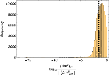
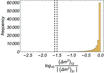
Figure 2: Distributions of the ratio $\log_{10}(\Delta m^{2}_{21}/|\Delta m^{2}_{3\ell}|)$ under the assumptions of NH (left panel) and IH (right panel) in Case I. Here, we impose no cut for the three mixing angles within the $3\sigma$ ranges. In the panels, the regions between the two vertical dashed black lines are $3\sigma$-favored for $\log_{10}(\Delta m^{2}_{21}/|\Delta m^{2}_{3\ell}|)$ [51]. Here we take $10^{5}$ points for each plot.

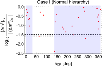
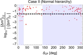
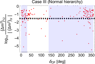
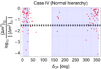
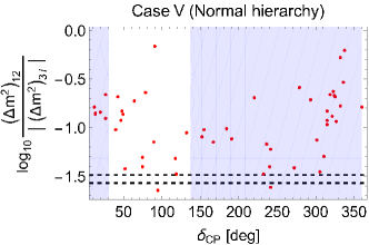
Figure 3: $\log_{10}(\Delta m^{2}_{21}/|\Delta m^{2}_{3\ell}|)$ – $\delta_{\text{CP}}$ distributions among the parameter points where the three mixing angles are within the $3\sigma$ regions. The pale blue regions show the $3\sigma$-favored region of $\delta_{\text{CP}}$ in a recent global fit [52]. It is noted that no region of $\delta_{\text{CP}}$ is $3\sigma$-disfavored in the results of the recent global fits [51, 53]. In each plot, the region between the two horizontal dashed black lines are $3\sigma$-favored for $\log_{10}(\Delta m^{2}_{21}/|\Delta m^{2}_{3\ell}|)$ [51].

3.3 Detailed analyses of each case

At first, we look whether the NH or IH case is preferred in our seesaw texture originating from the magnetized extra dimension with orbifolding. In Fig. 2, we show the distributions of the ratio defined as $\log_{10}(\Delta m^{2}_{21}/|\Delta m^{2}_{3\ell}|)$ in Case I, where NH and IH are assumed in the left and right panels, respectively. Here, we impose no cut for the three mixing angles within the $3\sigma$ ranges [51]. We immediately recognize that IH is highly disfavored since the corresponding range calculated from the global fit result in [51] is located far away from the peak of the obtained distribution. We found that the other cases have similar properties to Case I, where we can conclude that the IH case is disfavored in any case. Thereby hereafter, we only focus on the NH case in the five cases.

Next, we impose the $3\sigma$ conditions on the three mixing angles on the randomly generated configurations from the scattered parameters within the designated ranges as

$$\text{Re}\,\tau\in[-\pi,\pi],\qquad\text{Im}\,\tau\in(0,\pi],\qquad\rho_{2,3,4}\in[-1,-0.1]\cup[0.1,1],$$ (39)

where $10^{6}$ points are taken into account in each case individually. The correlations between $\log_{10}(\Delta m^{2}_{21}/|\Delta m^{2}_{3\ell}|)$ and $\delta_{\text{CP}}$ are described in Fig 3, where a few points (in each case) are $3\sigma$ acceptable also in the two values even though we take the severest result of such global fits among the one reported recently [52]. Also, we explicitly provide a sample in every case, summarized in Tab. 3, where they are generated when we adopt the parameters shown in Tab. 4. It is noted that the first four/two digits of $\tau$/$\rho_{2,3,4}$ looks sensitive to results in general.

In the rest of this section, we make a comment on a possible correlation between ${\rm Re}\,\tau$ and $\delta_{\rm CP}$. As shown in Fig. 3, we obtained only the $\sim 15$ number of candidates for allowed parameter points in total. This is due to the fact that the mass matrices stemming from (17) and (21) contain the Jacobi theta function that is defined in terms of an infinite summation over integers. Evaluating values of the function takes considerable time. Also, values of the Jacobi theta function are very sensitive to $\text{Im}\,\tau$ roughly like $e^{-c\,\text{Im}\,\tau}$ with a constant $c$. Therefore, we should carefully investigate effects originating from slight differences in $\text{Im}\,\tau$. For these difficulties in calculation time, we might ought to conclude that it is very difficult to extract strong predictions in the distributions of the realized CP phase concretely with keeping the current accuracy in the realized values of experimental measurements. However, we can get a clue for qualitative understanding for the CP phase through the following speculation. In the light of a previous study [50], one finds that the real part of the complex structure modulus generates non-zero physical values of the CP phase. In mass matrices stemming from flux compactification in quarks, we also observed considerable correlations between the value of ${\rm Re}\,\tau$ and the resulting (quark) CP violation phase. From these observations, we can make a suggestion that an observed region of neutrino CP phase at a confidence level may restrict an allowed range of ${\rm Re}\,\tau$. This point would lead to putting a constraint on types of possible mechanisms for moduli stabilization. It would be possible to reach strong predictions for the CP phase by combining our setups and appropriate moduli stabilizations in a future project. Nevertheless, being different from the quark case without brane-local term discussed in [50], the existence of the brane-local Majorana mass terms may lead to more complex pattens in the distributions of the realized CP angle, even though the coefficients of the mass terms are real as we assumed. Thereby, an exhaustive calculation with a very considerable calculation cost would be required for unveiling possible hidden patterns of the CP angle in the current system and we do not explore the detail of it in this manuscript.

4 Conclusion

In this paper, we have explored a new avenue to a natural explanation of the observed tiny neutrino masses with a dynamical realization of the three-generation structure in the neutrino sector. Under the magnetized background, matters have multiply-degenerated zero modes and the whole intergenerational structures (before diagonalization of mass matrices) are dynamically determined. In this sense, we can conclude that our scenario is favored in the concept of minimality, where no degree of freedom remains to deform part of an intergenerational structure by hand freely.

Another good feature in our story is that only one Higgs doublet is enough for reproducing measured configurations of neutrinos, being different from the case of the quarks which have been discussed in various previous works. On magnetized $T^{2}/Z_{2}$ orbifolds, four fixed points are observed, where we can write down Majorana-type mass terms of an $SU(2)_{L}$ singlet neutrino field, with different coefficients. Our numerical calculations have clarified that to find acceptable parameter configurations (where the three mixing angles and the mass ratio are within the $3\sigma$ ranges) is not exceedingly tough. As shown in Fig. 3, after a $10^{6}$-time random scan, a few valid cases are excavated in all of the five reasonable configurations in the magnetic fluxes and $Z_{2}$ parities (as summarized in Tab. 2).

Due to the complexity of the theta function and $Z_{2}$ orbifolding, physical CP-violating phase is realized [54, 55, 50]. When the Dirac CP phase in the Pontecorvo–Maki–Nakagawa–Sakata matrix is measured much more precisely, we may clarify what type of the fluxes and $Z_{2}$ parities is more favorable. Allowing complex coefficients in the brane-localized Majorana-type mass terms may lead to a successful leptogenesis scenario [56], where details of such a possibility can be discussed in a separated publication in future.

Before closing this section, we comment on the $U(1)$ gauge symmetry and its breaking that we have used to obtain the family structure in leptons. Since we focus only on the neutrino sector in this paper, we cannot decide whether such $U(1)$ symmetry is anomaly free or not in principle. The fate of the $U(1)$ symmetry would highly depend on philosophies in model embeddings. For example, multiple $U(1)$ symmetries are used in [24], and it is well known that multiple $U(1)$ symmetries appear even in the intersecting D-brane scenario [38] (and references therein). Even if the $U(1)$ is anomalous, there are possibilities to cancel it via the Green–Schwartz mechanism [57] in the case that the present scenario is realized by a more fundamental theory, e.g., the superstring theory. Another clue for breaking the $U(1)$ gauge symmetry is to add a scalar field for a spontaneous breakdown. In other words, the $U(1)$ breaking can be concluded after the total ultraviolet-completed setups are identified. Although we do not identify the total setups, the results we obtained can be typical patterns of neutrino mixings in flux compactification of toroidal orbifolds.

References

- [1] ATLAS Collaboration, G. Aad et al., “Observation of a new particle in the search for the Standard Model Higgs boson with the ATLAS detector at the LHC,” Phys.Lett. B716 (2012) 1–29, arXiv:1207.7214 [hep-ex].
- [2] CMS Collaboration, S. Chatrchyan et al., “Observation of a new boson at a mass of 125 GeV with the CMS experiment at the LHC,” Phys.Lett. B716 (2012) 30–61, arXiv:1207.7235 [hep-ex].
- [3] T2K Collaboration, K. Abe et al., “Observation of Electron Neutrino Appearance in a Muon Neutrino Beam,” Phys. Rev. Lett. 112 (2014) 061802, arXiv:1311.4750 [hep-ex].
- [4] NOvA Collaboration, P. Adamson et al., “First measurement of electron neutrino appearance in NOvA,” Phys. Rev. Lett. 116 no. 15, (2016) 151806, arXiv:1601.05022 [hep-ex].
- [5] Particle Data Group Collaboration, C. Patrignani et al., “Review of Particle Physics,” Chin. Phys. C40 no. 10, (2016) 100001.
- [6] P. Minkowski, “ at a Rate of One Out of Muon Decays?,” Phys. Lett. 67B (1977) 421–428.
- [7] T. Yanagida, “HORIZONTAL SYMMETRY AND MASSES OF NEUTRINOS,” Conf. Proc. C7902131 (1979) 95–99.
- [8] M. Gell-Mann, P. Ramond, and R. Slansky, “Complex Spinors and Unified Theories,” Conf. Proc. C790927 (1979) 315–321, arXiv:1306.4669 [hep-th].
- [9] R. N. Mohapatra and G. Senjanovic, “Neutrino Mass and Spontaneous Parity Violation,” Phys. Rev. Lett. 44 (1980) 912.
- [10] J. Schechter and J. W. F. Valle, “Neutrino Masses in SU(2) x U(1) Theories,” Phys. Rev. D22 (1980) 2227.
- [11] C. D. Froggatt and H. B. Nielsen, “Hierarchy of Quark Masses, Cabibbo Angles and CP Violation,” Nucl. Phys. B147 (1979) 277–298.
- [12] H. Ishimori, T. Kobayashi, H. Ohki, Y. Shimizu, H. Okada, and M. Tanimoto, “Non-Abelian Discrete Symmetries in Particle Physics,” Prog. Theor. Phys. Suppl. 183 (2010) 1–163, arXiv:1003.3552 [hep-th].
- [13] N. Arkani-Hamed and M. Schmaltz, “Hierarchies without symmetries from extra dimensions,” Phys. Rev. D61 (2000) 033005, arXiv:hep-ph/9903417 [hep-ph].
- [14] C. Bachas, “A Way to break supersymmetry,” arXiv:hep-th/9503030 [hep-th].
- [15] D. Cremades, L. Ibanez, and F. Marchesano, “Computing Yukawa couplings from magnetized extra dimensions,” JHEP 0405 (2004) 079, arXiv:hep-th/0404229 [hep-th].
- [16] A. P. Braun, A. Hebecker, and M. Trapletti, “Flux Stabilization in 6 Dimensions: D-terms and Loop Corrections,” JHEP 02 (2007) 015, arXiv:hep-th/0611102 [hep-th].
- [17] H. Abe, T. Kobayashi, and H. Ohki, “Magnetized orbifold models,” JHEP 0809 (2008) 043, arXiv:0806.4748 [hep-th].
- [18] Y. Fujimoto, T. Kobayashi, T. Miura, K. Nishiwaki, and M. Sakamoto, “Shifted orbifold models with magnetic flux,” Phys.Rev. D87 (2013) 086001, arXiv:1302.5768 [hep-th].
- [19] T.-H. Abe, Y. Fujimoto, T. Kobayashi, T. Miura, K. Nishiwaki, et al., “ twisted orbifold models with magnetic flux,” JHEP 1401 (2014) 065, arXiv:1309.4925 [hep-th].
- [20] T.-h. Abe, Y. Fujimoto, T. Kobayashi, T. Miura, K. Nishiwaki, and M. Sakamoto, “Operator analysis of physical states on magnetized orbifolds,” Nucl. Phys. B890 (2014) 442–480, arXiv:1409.5421 [hep-th].
- [21] W. Buchmuller, M. Dierigl, F. Ruehle, and J. Schweizer, “Chiral fermions and anomaly cancellation on orbifolds with Wilson lines and flux,” Phys. Rev. D92 no. 10, (2015) 105031, arXiv:1506.05771 [hep-th].
- [22] Y. Matsumoto and Y. Sakamura, “Yukawa couplings in 6D gauge-Higgs unification on with magnetic fluxes,” PTEP 2016 no. 5, (2016) 053B06, arXiv:1602.01994 [hep-ph].
- [23] T. Kobayashi and S. Nagamoto, “Zero-modes on orbifolds : magnetized orbifold models by modular transformation,” Phys. Rev. D96 no. 9, (2017) 096011, arXiv:1709.09784 [hep-th].
- [24] H. Abe, T. Kobayashi, H. Ohki, A. Oikawa, and K. Sumita, “Phenomenological aspects of 10D SYM theory with magnetized extra dimensions,” Nucl.Phys. B870 (2013) 30–54, arXiv:1211.4317 [hep-ph].
- [25] H. Abe, T. Kobayashi, K. Sumita, and Y. Tatsuta, “Supersymmetric models on magnetized orbifolds with flux-induced Fayet-Iliopoulos terms,” Phys. Rev. D95 no. 1, (2017) 015005, arXiv:1610.07730 [hep-ph].
- [26] H. Abe, T. Kobayashi, K. Sumita, and Y. Tatsuta, “Gaussian Froggatt-Nielsen mechanism on magnetized orbifolds,” Phys.Rev. D90 no. 10, (2014) 105006, arXiv:1405.5012 [hep-ph].
- [27] H. Abe, T. Kobayashi, H. Ohki, K. Sumita, and Y. Tatsuta, “Flavor landscape of 10D SYM theory with magnetized extra dimensions,” JHEP 1404 (2014) 007, arXiv:1307.1831 [hep-th].
- [28] T.-h. Abe, Y. Fujimoto, T. Kobayashi, T. Miura, K. Nishiwaki, M. Sakamoto, and Y. Tatsuta, “Classification of three-generation models on magnetized orbifolds,” Nucl. Phys. B894 (2015) 374–406, arXiv:1501.02787 [hep-ph].
- [29] Y. Fujimoto, T. Kobayashi, K. Nishiwaki, M. Sakamoto, and Y. Tatsuta, “Comprehensive analysis of Yukawa hierarchies on with magnetic fluxes,” Phys. Rev. D94 no. 3, (2016) 035031, arXiv:1605.00140 [hep-ph].
- [30] W. Buchmuller, M. Dierigl, F. Ruehle, and J. Schweizer, “Split symmetries,” Phys. Lett. B750 (2015) 615–619, arXiv:1507.06819 [hep-th].
- [31] W. Buchmuller and J. Schweizer, “Flavor mixings in flux compactifications,” Phys. Rev. D95 no. 7, (2017) 075024, arXiv:1701.06935 [hep-ph].
- [32] W. Buchmuller and K. M. Patel, “Flavor physics without flavor symmetries,” Phys. Rev. D97 no. 7, (2018) 075019, arXiv:1712.06862 [hep-ph].
- [33] M. Ishida, K. Nishiwaki, and Y. Tatsuta, “Brane-localized masses in magnetic compactifications,” Phys. Rev. D95 no. 9, (2017) 095036, arXiv:1702.08226 [hep-th].
- [34] T. Higaki and Y. Tatsuta, “Inflation from periodic extra dimensions,” JCAP 1707 no. 07, (2017) 011, arXiv:1611.00808 [hep-th].
- [35] W. Buchmuller, M. Dierigl, F. Ruehle, and J. Schweizer, “de Sitter vacua from an anomalous gauge symmetry,” Phys. Rev. Lett. 116 no. 22, (2016) 221303, arXiv:1603.00654 [hep-th].
- [36] W. Buchmuller, M. Dierigl, F. Ruehle, and J. Schweizer, “de Sitter vacua and supersymmetry breaking in six-dimensional flux compactifications,” Phys. Rev. D94 no. 2, (2016) 025025, arXiv:1606.05653 [hep-th].
- [37] L. E. Ibanez and A. M. Uranga, “Neutrino Majorana Masses from String Theory Instanton Effects,” JHEP 03 (2007) 052, arXiv:hep-th/0609213 [hep-th].
- [38] L. E. Ibanez and A. M. Uranga, String theory and particle physics: An introduction to string phenomenology. Cambridge University Press, 2012.
- [39] Y. Hamada, T. Kobayashi, and S. Uemura, “Flavor structure in D-brane models: Majorana neutrino masses,” JHEP 05 (2014) 116, arXiv:1402.2052 [hep-th].
- [40] T. Kobayashi, Y. Tatsuta, and S. Uemura, “Majorana neutrino mass structure induced by rigid instantons on toroidal orbifold,” Phys. Rev. D93 no. 6, (2016) 065029, arXiv:1511.09256 [hep-ph].
- [41] H. Abe, K.-S. Choi, T. Kobayashi, and H. Ohki, “Three generation magnetized orbifold models,” Nucl.Phys. B814 (2009) 265–292, arXiv:0812.3534 [hep-th].
- [42] J.-M. Frere, M. Libanov, and F.-S. Ling, “See-saw neutrino masses and large mixing angles in the vortex background on a sphere,” JHEP 09 (2010) 081, arXiv:1006.5196 [hep-ph].
- [43] A. Pilaftsis, “Leptogenesis in theories with large extra dimensions,” Phys. Rev. D60 (1999) 105023, arXiv:hep-ph/9906265 [hep-ph].
- [44] E. Dudas, C. Grojean, and S. K. Vempati, “Classical running of neutrino masses from six dimensions,” arXiv:hep-ph/0511001 [hep-ph].
- [45] B. A. Dobrescu and E. Poppitz, “Number of fermion generations derived from anomaly cancellation,” Phys. Rev. Lett. 87 (2001) 031801, arXiv:hep-ph/0102010 [hep-ph].
- [46] C. S. Lim, “The implication of gauge-Higgs unification to the hierarchical fermion masses,” arXiv:1801.01639 [hep-ph].
- [47] W. Buchmuller, M. Dierigl, E. Dudas, and J. Schweizer, “Effective field theory for magnetic compactifications,” JHEP 04 (2017) 052, arXiv:1611.03798 [hep-th].
- [48] D. M. Ghilencea and H. M. Lee, “Wilson lines and UV sensitivity in magnetic compactifications,” JHEP 06 (2017) 039, arXiv:1703.10418 [hep-th].
- [49] H. Abe, T. Kobayashi, Y. Tatsuta, and S. Uemura, “D-brane instanton induced terms and their hierarchical structure,” Phys. Rev. D92 no. 2, (2015) 026001, arXiv:1502.03582 [hep-ph].
- [50] T. Kobayashi, K. Nishiwaki, and Y. Tatsuta, “CP-violating phase on magnetized toroidal orbifolds,” JHEP 04 (2017) 080, arXiv:1609.08608 [hep-th].
- [51] I. Esteban, M. C. Gonzalez-Garcia, M. Maltoni, I. Martinez-Soler, and T. Schwetz, “Updated fit to three neutrino mixing: exploring the accelerator-reactor complementarity,” JHEP 01 (2017) 087, arXiv:1611.01514 [hep-ph].
- [52] F. Capozzi, E. Di Valentino, E. Lisi, A. Marrone, A. Melchiorri, and A. Palazzo, “Global constraints on absolute neutrino masses and their ordering,” Phys. Rev. D95 no. 9, (2017) 096014, arXiv:1703.04471 [hep-ph].
- [53] S. Gariazzo, M. Archidiacono, P. F. de Salas, O. Mena, C. A. Ternes, and M. Tórtola, “Neutrino masses and their ordering: Global Data, Priors and Models,” arXiv:1801.04946 [hep-ph].
- [54] C. S. Lim, “CP violation in higher dimensional theories,” Phys. Lett. B256 (1991) 233–238.
- [55] C. S. Lim, N. Maru, and K. Nishiwaki, “CP Violation due to Compactification,” Phys. Rev. D81 (2010) 076006, arXiv:0910.2314 [hep-ph].
- [56] M. Fukugita and T. Yanagida, “Baryogenesis Without Grand Unification,” Phys. Lett. B174 (1986) 45–47.
- [57] M. B. Green and J. H. Schwarz, “Anomaly Cancellation in Supersymmetric D=10 Gauge Theory and Superstring Theory,” Phys. Lett. 149B (1984) 117–122.