The Cosmic-Ray Spectra:
News on their Knees

Abstract

In a comprehensive model of Cosmic Rays (CRs) proposed a decade ago, the energies of the spectral “knees” of the various CR species were predicted to be proportional to mass, rather than charge. The model also predicts the knees to occur at an energy of two to four million times the particle’s rest mass. Recent data allow one to verify this prediction, particularly for Fe and lighter-nuclei CRs. But the most stringent test involves the putative knee in the CR electron spectrum, since the mass ratio of electrons to protons (and nuclei) is so very different from their charge ratio(s). Very recent results on the spectra of positrons and electrons at the highest measured energies corroborate the existence of an electron knee, with the expected shape and at the predicted energy.

I Introduction

Cosmic Rays (CRs) occupy a very peculiar niche in physics. Though they were discovered more than a century ago, there is no acceptable and accepted theory that describes them. This is in spite of the fact that there is no reason to believe that the understanding of CRs would require any revolutionary ingredients. And this applies not only to protons and other nuclei, but also to CR electrons and positrons, for which claims of “physics beyond the standard model” abound.

A significant contribution to the lack of a generally trusted CR theory is that the number of correct predictions in the field is impressively small. One exception is the prediction by Giuseppe Cocconi and Philip Morrison Cocconi ; Morrison that the magnetic field of the galaxy would not be able to confine CRs of energy exceeding ${\rm Z}\,(3\times 10^{9})$ GeV, with Z the CR’s charge. Some spectral feature is then expected at such an energy. This, for $\rm Z=1$, turns out to be seen as the “ankle” in the all-particle spectrum. Auger has recently observed a dipolar asymmetry in the incoming directions of CRs of energy above $8\times 10^{9}$ GeV, pointing in the sky in a direction very different to that of the galactic center Auger . Cocconi and Morrison were right.

Another beautifully simple prediction is the “GZK cutoff” at energies exceeding ${\rm A}\,(5\times 10^{10})$ GeV, with A the CR’s mass number GZK . Ultra-High Energy Cosmic Rays with energies amply exceeding the proton’s GZK limit are observed and their composition is unknown. The original GZK cutoff reflects the pion-production threshold on the cosmic microwave and infrared backgrounds. The understanding of the highest-energy CR flux is complicated by the fact that photo-dissociation of primary CR nuclei is relevant at similar energies.

A decade ago a Cannon-Ball (CB) model of CRs DP was elaborated DD2008 . The model is very economic, in the sense of having only one free parameter to be fit to the data. Its remaining degrees of freedom concern “priors”, information to be gathered from observations independent from the model. With choices of the priors in their allowed range, the model was shown to accurately describe all properties of (primary, non-solar) CRs. New data allow one to discuss a prediction of the CB model, concerning the knees in the spectra of the fluxes of individual nuclei and electrons. The prediction turns out to be right.

The CB model of Gamma-Ray Bursts and X-Ray Flashes SD ; GRB1 ; DD ; AGoptical ; AGradio ; DDDXRF (collectively, GRBs), CRs, the gamma background radiation DDGBR , cooling flows CDD and neutron-star mergers NS cannot be accused of being unjustifiably popular. For that reason, I summarize in an appendix the information required to understand the basis for the predictions of the CB model concerning the CR knees.

Suffice it to say at this point that core-collapse supernovae (SNe) produce highly relativistic jets of “cannonballs” of ordinary matter. These CBs, colliding with the constituents of the interstellar medium (ISM), promote them to CR energies. GRBs and their afterglows are also generated by CBs launched by SNe, when accurately pointing to the observer from a distant galaxy. The successful CB-model description of GRBs allows one to extract the information required to predict the properties of CRs.

II The Knees

About a decade ago the data on the separate spectra of protons and He and Fe nuclei were the ones depicted in Fig. (1). Also shown in this figure are various CB-model descriptions of the data, corresponding to choices of the priors within their respective ranges DD2008 . These data showed a significant knee for protons, and an indication of a He knee. The measurements did not extend high enough in energy to reflect a potential Fe knee.

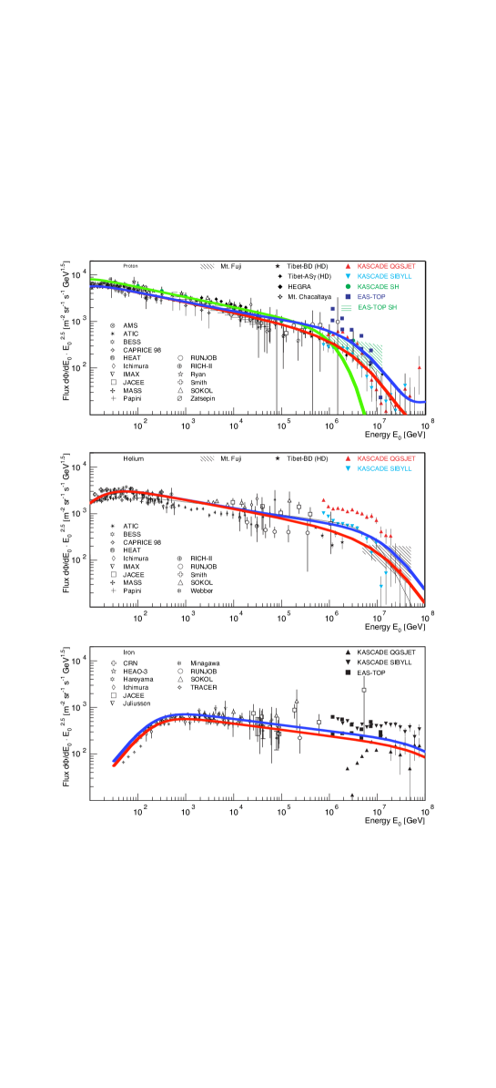
Figure 1: Early data Hor on the p, He and Fe spectra (times $E^{2.5}$) and their early CB-model description DD2008 . The red and blue curves indicate the sensitivity to contributions subdominant in the plotted energy range, with their priors chosen within their ranges. The green curve illustrates the choice of a very narrow distribution of CB’s initial Lorentz factors. The compilation of data was at the time kindly provided to us by K.H. Kampert.

In the range of energies shown in Fig. (1) the dominant contribution to the CB-model spectra is the scattering by a moving CB of the constituents of the ISM, previously ionized by the GRB’s $\gamma$ rays. The red and blue curves indicate the sensitivity to subdominant contributions: the extragalactic CR flux and the CRs having been accelerated in a CB’s inner magnetic field. These small contributions are neglected in what follows; they have an inconsequential impact on the discussion of the spectral knees, on which we are interested here.

The curves in Fig. (1) reflect the fact that the CB model correctly describes the CR data at all energies including, though not shown in the figure, the data at the highest and smallest measured energies. In the low-energy domain the CB-model description of the spectra is not as simple as for relativistic energies DD2008 . For the sake of expedience in discussing the knees, I shall only use here the CB-model’s results for very relativistic CRs.

Let $\gamma_{0}$ be the initial Lorentz factor (LF) with which a given CB is ejected in a supernova event. A distribution of $\gamma_{0}$ values, $D(\gamma_{0})$ –extracted from the analysis of GRBs and their afterglows– is shown in Fig. (2). It peaks at $\bar{\gamma}_{0}$ slightly larger than $10^{3}$, above which it falls abruptly. The data at $\gamma_{0}<\bar{\gamma}_{0}$ may be under-represented due to observational selection effects (smaller GRB fluxes), but only the high-$\gamma_{0}$ part of $D(\gamma_{0})$ is relevant to the location and shape of the CRs knees.

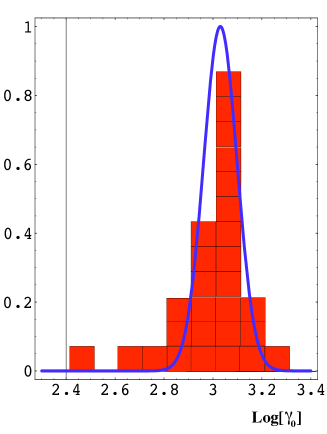
Figure 2: The distribution $D(\gamma_{0})$ of initial Lorentz factors of CBs, extracted from data on GRBs and their afterglows DD2008 . The blue curve is a log-normal description of the data.

Soon after its launching, a CB expands to a point where its density is low enough for it to become transparent –in the sense of its individual constituents and the ones of the ISM it encounters not to scatter significantly. But a CB has an inner turbulent magnetic field, as explained in the Appendix. This field captures and scatters the charged ISM constituents. As the CB expands and slows down in its trajectory, this results in the ISM particles being re-emitted by the CB as CRs with a distribution of their LFs, $\gamma_{{}_{\rm CR}}$:

$${dF\over d\gamma_{{}_{\rm CR}}}\propto n_{{}_{\rm A}}\,\gamma_{{}_{\rm CR}}^{-\beta_{s}}\,\Theta[2\,\gamma_{0}^{2}-\gamma_{{}_{\rm CR}}],\;\;\;\beta_{s}={13\over 6}\approx 2.17,$$ (1)

with $n_{{}_{\rm A}}$ the abundance of the ISM nuclei of nucleon number A that the CB collides with DD2008 .

The upper limit $\gamma_{{}_{\rm CR}}\leq 2\,\gamma_{0}^{2}$ is easy to understand. Consider a freshly ejected CB in its rest frame. The incoming ISM particles reach it with a LF $\gamma_{0}$. The ones elastically back-scattered have in the CB’s rest frame a LF $\gamma_{0}$, the mass of the CB being so much larger than the energy of the ISM projectile. Lorentz-boost these scattered particles back to the ISM rest system. Their LF there, the maximum possible one, is $2\,\gamma_{0}^{2}$. A relativistic racket is an incredibly efficient accelerator!

The $\Theta$ function in Eq. (1), converted to a limit on energy, (in $c=1$ units) is:

$$E_{\rm max}=2\,\gamma_{0}^{2}\,M.$$ (2)

This is the key prediction: there must be a spectral feature in the different species of CRs at an energy of $\sim(2\,{\rm to}\,4)\!\times\!10^{6}$ their mass. Since the distribution of values of $\gamma_{0}$ is not quite a $\delta$ function and “elastic” scattering is dominant only up to $E_{\rm max}$, the spectral feature is a knee.

Based on Fermi’s hypothesis that CRs are accelerated by moving shocks of magnetized material, the conventional wisdom is that features in the CR spectra of individual nuclides ought to have energies scaling with charge. But, at least for the knees’ energies there is, to my knowledge, no equivalent to the $2\,\gamma_{0}^{2}$ proportionality factor of Eq. (2).

The expression $dF/d\gamma_{{}_{\rm CR}}\propto\gamma_{{}_{\rm CR}}^{-\beta_{s}}$ of Eq. (1) is not yet a prediction for a CR spectrum. At energies well below the ankle, CRs are confined and accumulated by the Galaxy’s magnetic field for a time, $\tau_{\rm conf}$, that depends on their charge, Z, and momentum, $p$. An observed spectrum $F_{{}_{\rm CR}}$ and the source spectrum $F$ are therefore related by:

$$\!\!F_{{}_{\rm CR}}\propto\tau_{\rm conf}\,F,\;\;\;\tau_{\rm conf}=\tau_{0}\,({\rm Z}\,p_{0}/p)^{\beta_{\rm conf}};$$

$$\tau_{0}\sim(2-3)\times 10^{7}\,{\rm years},\;\;\;{\beta_{\rm conf}}\sim 0.6\pm 0.1,$$ (3)

with $p_{0}\sim 1$ GeV and $\tau_{0}$ and ${\beta_{\rm conf}}$ estimated from observations of astrophysical and solar plasmas and corroborated by measurements of the relative abundances of secondary CR isotopes CONFI .

Recent measurements of the B/C ratio AMS imply, at low rigidity ($R$) smaller values of $\beta_{\rm conf}$ than given in Eq. (3), see Fig. 2 in AMS . As theoretically expected, $\beta_{\rm conf}(R)$ flattens as $R$ increases. The measured value at the highest-rigidity point ($R=860$ GV) is $.52\pm.13$. The rigidities of the knees discussed here are $\sim 10^{3}$ times larger, and the primary CR spectra are adequately described by single power laws for more than three orders of magnitude below their knees, see Fig. (1). It is therefore reasonable, as we do in what follows, to adopt $\beta_{\rm conf}=0.6$, compatible with the results of CONFI and AMS .

An inspection of Fig.(4) below indicates that a value of $\beta_{\rm conf}$ smaller than 0.6 would result in a slightly better description of the data. A reason to use an “old” value of $\beta_{\rm conf}$ is that this paper deals with the predictions of an “old” theory, rather than a description of recent data.

II.1 CR abundances

Let us pause to check whether we are on the right track. It is customary to discuss the composition of CR nuclei at a fixed energy $E_{{}_{\rm A}}=1$ TeV. This energy is relativistic ($p\simeq E$), below the corresponding knees for all A, and in the domain wherein the fluxes are well approximated by a power law with the index $\beta_{\rm th}\!=\!\beta_{s}\!+\!\beta_{\rm conf}\!\simeq\!2.77$, predicted by combining Eqs. (1) and (3). Expressed in terms of energy ($E_{{}_{\rm A}}\!\propto\!{\rm A}\,\gamma$), read below the knee of Eq. (2) and modified by confinement as in Eq. (3), Eq. (1) becomes:

$${dF_{\rm obs}\over dE_{{}_{\rm A}}}\propto{n}_{{}_{\rm A}}\,{\rm A}^{\beta_{\rm th}-1}\,E_{{}_{\rm A}}^{-\beta_{\rm th}},\;\;\;X_{{}_{\rm CR}}({\rm A})={{n}_{{}_{\rm A}}\over{n}_{p}}\,{\rm A}^{1.77},$$ (4)

with ${n}_{{}_{\rm A}}$ an average ISM abundance and $X_{{}_{\rm CR}}({\rm A})$ the CR abundances relative to H, at fixed $E_{{}_{\rm A}}$ DD2008 .

The results of Eq. (4), for input ${n}_{{}_{\rm A}}$’s in the ‘superbubbles’ wherein most SNe occur, are shown in Fig. (3). In these regions, the abundances are a factor $\sim\!3$ more ‘metallic’ than solar. The data snugly reproduce the large enhancements of the heavy-CR relative abundances, in comparison with solar or superbubble abundances (e.g. ${\rm A}^{1.77}\!=\!1242$ for Fe).

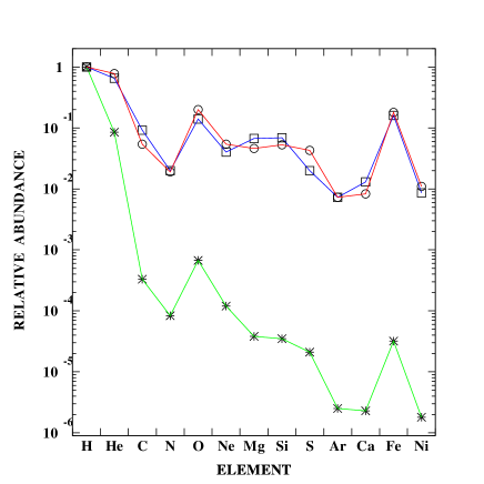
Figure 3: The relative abundances of primary CR nuclei, from H to Ni around 1 TeV BWS . The stars (joined by green lines) are solar-ISM abundances GS . The circles (joined in red) are the predictions, with input superbubble abundances. The squares (joined in black) are the CR observations.

Within the large uncertainties of its priors (supernova rates, confinement time and volume) the CB model accounts for the normalization of the all-particle CR flux, dominated by protons. With smaller uncertainties in the input priors, we have seen that the relative abundances of the various primary CR nuclei are fairly well reproduced. Consequently, in comparing theory and observations of the CR fluxes of each given nuclide, we shall take the liberty of fitting “by eye” the overall normalization of the theory to the data.

The CB model of CRs is a model of the origin and spectra of primary CRs. Once one has an (alleged) understanding of the injection spectrum of primaries arriving not so far from the Earth, the understanding of secondaries is common to all models and it is relatively well understood, at least at the qualitative level and at all but the smallest rigidities. Secondaries are not a clear-cut tool to distinguish different models of the origin of CRs.

The secondary to primary ratios (see, for instance, Fig. 1 of AMS for the B/C ratio) are seen –and theoretically understood JSM – to decrease very fast with energy. At the energies of interest to the CR knees (three orders of magnitude above the highest measured rigidities, of order $2\times 10^{3}$ GV) the depletion of the primary CRs cannot be an effect greater than few tens of a percent. This is certainly negligible relative to the dominant uncertainties in the CB-model priors, such as the all-particle flux normalization.

III Back to the spectral knees

A prior in discussing the position and shape of the knees is $D(\gamma_{0})$, the distribution of initial LFs of CBs, of which an example was given in Fig. (2). Convoluted with $D(\gamma_{0})$ and as a function of energy, Eq. (1) becomes:

$$F_{{}_{\rm A}}=E_{{}_{\rm A}}^{-\beta_{\rm th}}\;{\rm Knee}(E_{{}_{\rm A}}),$$

$$\beta_{\rm th}=\beta_{s}+\beta_{\rm conf}\sim 2.77,$$

$${\rm Knee(E_{{}_{\rm A}})}\equiv\int_{E_{{}_{\rm A}}/[2M({\rm A})]}^{\infty}D(\gamma_{0}^{2})\,d\gamma_{0}^{2}$$ (5)

The most recent data on the CR spectra of individual elements are shown in Fig. (4). The CB-model curves are colored and correspond to a log-normal distribution:

$$D(x)={\rm Exp}(-[(x-x_{0})/c]^{2});$$

$$x\equiv{\rm Log}_{10}[\gamma_{0}^{2}],\;\;x_{0}=6.3,\;\;c=0.5,$$ (6)

which results in the red curve that satisfactorily describes the proton’s knee (this function peaks at a value of ${\rm Log}_{10}[\gamma_{0}]$ some 4% larger than the prior shown in Fig. (2) and is about twice as large). The blue curve beyond the knee corresponds to a contribution, not needed for the current discussion, of protons accelerated within the CBs DD2008 (for all CR nuclei, this contribution improves the agreement between theory and data, as in Fig. (1), at energies well below the knee). The curves labeled DD2008 in Fig. (4) correspond to the prediction of Eqs.(5) with $\rm Knee(E_{{}_{\rm A}})=1$, i.e. no knee.

The next CR nuclide shown in Fig. (4) is Fe since, should one trust the recent KASKADE-Grande data Hor2 more than previous ones, they provide the best-measured knee. The shape of the red curve is this time completely predicted, since the $D(\gamma_{0})$ prior has been chosen to describe the proton’s knee. Once again, the result is based on the simple kinematical fact that in the CB model the knee positions scale with mass, not charge. The dotted blue curve corresponds to the later case. Its exclusion is not as clear-cut as the figure seems to imply. One could have fit $D(\gamma_{0})$ to the Fe knee to predict the proton data. Since these do not appear to be so precise, the exclusion of the generally assumed dependence on charge would have been a wee bit less convincing.

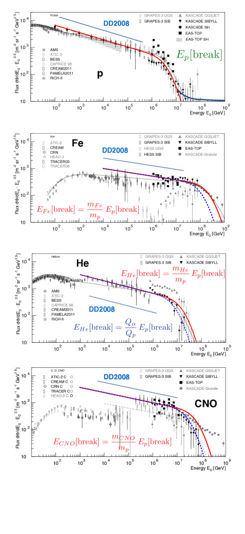
Figure 4: The spectra (times $E^{2.5}$) of primary CR nuclides: p, Fe, He and CNO Hor2 . The relative positions of their knees are predicted by the CB model (red lines). Their exact absolute positions and shapes are obtained by adjusting a prior (the distribution $D(\gamma_{0})$ of initial CB Lorentz factors) within its uncertainties. The dashed blue lines correspond to the hypothesis that the knees scale with charge, not mass. The “DD2008” lines are the expected spectral slopes DD2008 , to be continued to higher energies in the absence of knees. The (red) CB-model results are totally satisfactory, but for the CNO group, whose spectrum as measured by KASKADE-Grande Hor2 is somewhat peculiar.

The data on He shown in Fig. (4) display a much clearer knee than the older ones in Fig. (1). Once again, they do not establish a distinction between knees scaling with charge or mass. Finally, the data on the CNO group also have a knee, whose shape makes one wonder.

IV The electron knee

The mass ratio of Fe to protons is $\sim 56$, while their charge ratio is 26. The relatively small ratio of these numbers ($\sim 2.15$) –combined with the errors in the data and their spread– are such that we could not establish a clear preference between charge and mass in the positions of their respective spectral knees. A comparison between electrons and protons, with a charge ratio of $[-]1$ and a mass ratio of $\sim 1832$, could prove decisive.

The spectral index for electrons of energies close to their putative knee is not $\beta_{\rm th}\sim 2.77$ as in Eq. (5) but $\beta_{\rm e}=\beta_{\rm th}+1$. The reason DD2008 is that in this energy domain electrons (and positrons) efficiently lose energy by synchrotron radiation in the Galaxy’s magnetic field and inverse Compton scattering on ambient photons. The knee function in Eq. (5) only requires the substitution of $M({\rm A})$ for $m_{\rm e}$.

The currently available relevant data are for the sum of $e^{+}$ and $e^{-}$ fluxes. The most conservative assumption is that positrons are CR secondaries, generated in CR collisions with the ISM, producing pions (or kaons) with a decay chain $\pi^{+}\,({\rm or}\,K^{+})\,\to\mu^{+}\,\nu$, $\mu^{+}\to e^{+}\,\nu\,\bar{\nu}$. The same collisions generate secondary electrons with a similar energy distribution, but in smaller quantities, due to the CR nuclei and their ISM targets being positively charged. At a fixed energy the ratio of the secondary electron flux to the one of positrons ought to be $\sim 0.74$, the measured $\mu^{+}/\mu^{-}$ ratio DaDa .

In testing the prediction for the electron knee, I add to its spectrum the relatively small contribution of secondary $e^{+}$ and $e^{-}$ fluxes, to be able to compare with the current data up to the highest measured energies. For the secondary $e^{+}$ flux I use the expressions in DaDa , which are conservative (in the sense of the previous paragraph) and snuggly fit the data.

Two sets of data and the CB-model fit are shown in the busy Fig. (5). This is a (one-parameter) fit in the sense that we have not attempted to predict in the CB model the absolute normalization of the CR electron spectrum. The top of Fig. (5) contains a relatively new set of data in a log-log plot, like previous figures. The lower part of the figure is a linear-log plot, thus the (apparently) dissimilar shapes of the differently colored lines, which are precisely the same functions in the two plots.

The upper part of Fig. (5) shows that there is indeed an electron knee at the energy predicted by the CB model. Its shape is also compatible with the theoretical prediction. The lower part of Fig. (5) thickens the plot. The AMS-02 data are incompatible with the others and, since they do not reach the highest-measured energies, cannot significantly distinguish a knee from its absence. Finally, the data reaching the highest energies, from HESS and DAMPE, agree with the presence of the primary electron knee, with its predicted position and shape.

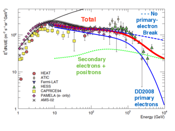
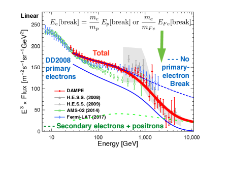
Figure 5: Top: Relatively recent data on the $e^{+}+\,e^{-}$ CR spectra (times $E^{3}$), on a log-log scale rpp . The spectral knee predicted by the CB model in the primary $e^{-}$ spectrum is clearly seen. Bottom: More recent data on a linear-log scale Dampe . The knee is very conspicuosly observed in the DAMPE and HESS results, which reach the highest energies. The dashed green curves are the secondary $e^{+}+\,e^{-}$ CR spectra. The blue curves are the spectra of primary electrons (with a fitted normalization). The dotted blue curves describe a would-be theory with no knee. The thick red curve is the complete CB-model result.

V Summary and Conclusions

In the CB model there must be a knee in the spectra of primary CR nuclides and electrons at an energy of (2 to 4) $\times\,10^{6}$ times the particle’s rest energy. A decade ago the prediction was only (succesfully) testable for protons and –to some extent– for Fe, whose spectral knee was already indirectly observable as the “second knee” in the all-particle spectrum DD2008 .

Recent data allow one to test the cited prediction. It turns out to be right for protons, He and Fe. The measurement errors, however, are insufficient to decide whether the observed knees scale with mass or charge (the second choice would relate the relative positions of the knees, but does not predict their absolute energies).

Clearly, a decisive test would involve a measurement of the primary electron spectrum, since the charge ratio of protons to electrons is extremely different from their mass ratio: $\sim 1832$; not to speak of the mass ratio of Fe to electrons: five orders of magnitude! There is not yet a measurement of the electron spectrum up to its predicted knee. But measurements of the separate $e^{+}$ and $e^{-}$ spectra exist, up to energies a bit below that of the predicted primary-electron knee.

In a theory not invoking non-standard physics, the $e^{+}$ CRs are secondary, and accompanied by a predictable amount of secondary $e^{-}$’s. The individual lepton spectra are very well described in such a theory DaDa . With its help, and the CB-model prediction for the primary $e^{-}$ spectrum, I have argued that the CB-model’s knee is observed. This involves a modest extrapolation of the cited theory of secondary spectra, but there is no reason to expect a break in these spectra, generated by collisions between higher-energy CR nuclei and the ISM, and convoluted with the corresponding very broad spectra of secondary pions (and kaons) and the chain of their decay products. Moreover, the contribution of the secondary $e^{+}+\,e^{-}$ to the total flux is, up to the $e^{-}$ knee, quite negligible, see Fig. (5).

All in all, the CB-model’s prediction of a knee in the CR spectra of primary hadrons and electrons turns out to be correct. The only caveats are related to peculiarities of the data, see the CNO spectrum of Fig. (4) and the disagreements between experiments in the lower part of Fig. (5). Perhaps the correct conclusion at this point would be the one attributed to Eddington: Never trust an experiment until it has been confirmed by theory.

VI Added Note

Right after the original version of this paper was posted, relevant new data on the $e^{+}+\,e^{-}$ spectrum were published by CALET CALET . They are shown in Fig.(6). Interestingly, they agree with the AMS data shown in the lower panel of Fig.(5). But they extend to higher, knee-sensitive, energies.

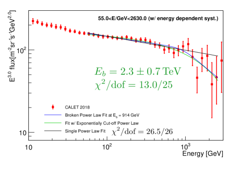
Figure 6: CALET data on the $e^{+}+\,e^{-}$ spectrum. The black curve is a single power-law. The green curve includes an exponential break.

The black single power-law fit of Fig.(6) has $\chi^{2}/\rm dof=26.5/26$. The green curve is a fit with $\chi^{2}/\rm dof=13.0/25$ and an exponential break at $E_{b}=2.3\pm 0.7$ TeV. The only daringly precise prediction for the position of the electron knee –also an exponential cutoff, as in Eqs.(5, 6)– is $E_{b}=2.3$ TeV ADRprecise . This coincidence is intriguing, but the difference in the fit qualities of the single-power-law and the exponentially-cutoff fits is, by itself, insufficient to justify any strong claims.

Acknowledgment: A. De Rújula acknowledges that this project has received funding/support from the European UnionÕs Horizon 2020 research and innovation programme under the Marie Sklodowska-Curie grant agreement No 690575. I am particularly indebted to Shlomo Dado and Arnon Dar for discussions, a long-time collaboration and for lending me their analytic expressions for the fluxes of CR positrons and secondary electrons.

Appendix: The CB model of GRBs and CRs

Jets are emitted by many astrophysical systems, such as Pictor A, shown in Fig. (7). Its active galactic nucleus is discontinuously spitting something that, seen in X-rays, does not appear to expand sideways before it stops and blows up, having by then travelled almost $10^{6}$ light years. Many such systems have been observed. They are relativistic: the Lorentz factors (LFs) $\gamma\!\equiv\!E/(mc^{2})$ of their ejecta are of ${\cal{O}}(10)$. The mechanism responsible for these ejections, due to episodes of violent accretion into a very massive black hole, is not understood in detail.

The radio signal in Fig. (7) is the synchrotron radiation of Ôcosmic-rayÕ electrons Pictor . Electrons and nuclei were scattered by the CBs of Pictor A, which encountered them at rest in the intergalactic medium, kicking them up to high energies. Thereafter, these particles diffuse in the ambient magnetic fields (that they contribute to generate) and the electrons radiate.

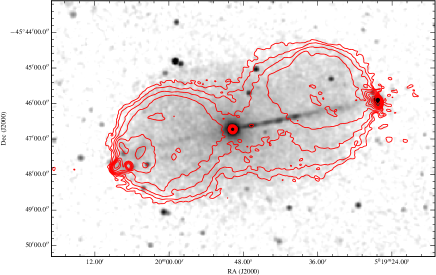
Figure 7: The quasar Pictor A. A superposition of an X-ray image and the (red) contours of the radio emission Pictor .

In our galaxy there are ‘micro-quasars’, whose central black hole’s mass is a few $M_{\odot}$. The best studied GRS is GRS 1915+105. A-periodically, about once a month, this object emits two oppositely directed cannonballs, travelling at $v\sim 0.92\,c$. When this happens, the continuous X-ray emissions —attributed to an unstable accretion disk— temporarily decrease. Atomic lines of many elements have been seen in the CBs of $\mu$-quasar SS 433 SS433 . Thus, at least in this case, the ejecta are made of ordinary matter, and not of a fancier substance, such as $e^{+}e^{-}$ pairs.

The ‘cannon’ of the CB model is analogous to the ones of quasars and $\mu$-quasars. In the core-collapse responsible for a stripped-envelope SNIc event, due to the parent star’s rotation, an accretion disk is produced around the newly-born compact object, by stellar material originally close to the surface of the imploding core, or by more distant stellar matter falling back after the shock’s passage. A CB made of ordinary-matter plasma is emitted, as in microquasars, when part of the accretion disk falls abruptly onto the compact object. Long-duration GRBs and non-solar CRs are produced by these jetted CBs.

A summary of the CB model of GRBs and XRFs is given in Fig. 8. The ‘inverse’ Compton scattering (ICS) of light by electrons within a CB produces a highly forward-collimated beam of higher-energy photons. The target light is in a temporary reservoir: the glory, an ÒechoÓ (or ambient) light from the SN, permeating the Òwind-fedÓ circumburst density profile, previously ionized by the early extreme UV flash accompanying a SN explosion, or by the enhanced UV emission that precedes it.

Seen close to the CB’s direction of motion, the beam of $\gamma$-rays is a pulse of a GRB. Not so close, it is the pulse of an XRF. To agree with observations, CBs must be launched with LFs, $\gamma_{0}\!\sim\!10^{3}$, and baryon numbers $N_{{}_{\rm B}}\!=\!{\cal{O}}(10^{50})$, corresponding to $\sim\!1/2$ of the mass of Mercury, a miserable $\sim\!10^{-7}\,M_{\odot}$.

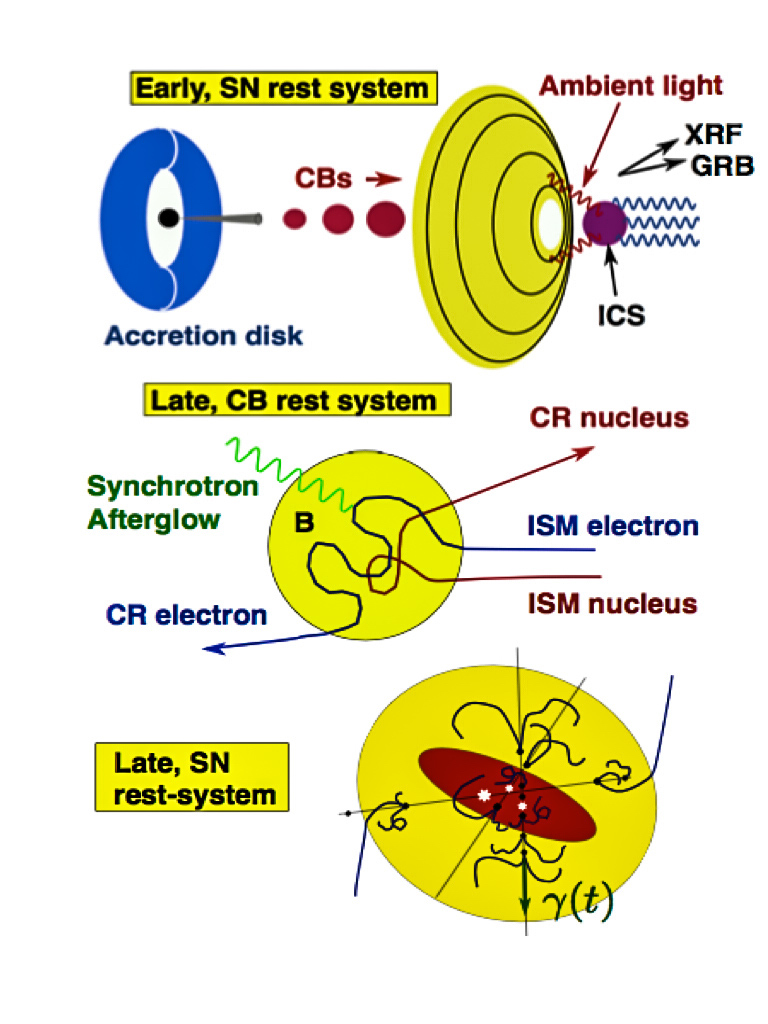
Figure 8: The CB model of GRBs, XRFs and CRs. A core-collapse SN results in a (black) compact object, a (blue) fast-rotating torus of non-ejected material and a (yellow) shell of non-relativistic ejecta. Matter (not shown) episodically accreting into the central object produces two collimated beams of (brown) CBs; some of the ‘Northern’ ones are depicted. As the CBs move through the glory of non-radial light surrounding the star, they forward Compton up-scatter its photons to GRB or XRF energies, depending on how close the line of sight is to the CBs’ direction. Each CB produces a GRB or XRF ‘pulse’. Later, a CB gathers and scatters ISM particles, which “collide” with its inner magnetic field. When re-emitted, these particles are boosted by the CB’s motion: they have become CRs. The synchrotron radiation of the gathered electrons is the late AG of the GRB or XRF. As a CB’s collisions with the ISM slow it down, it generates CRs along its trajectory, in the galaxy and its halo. These CRs diffuse thereafter in the local magnetic fields.

The simple kinematics describing a narrow beam of GRB or XRF photons –viewed at different angles– suffice to predict all observed correlations between pairs of prompt observables, e.g. photon fluence, energy fluence, peak intensity and luminosity, photon energy at peak intensity or luminosity, and pulse duration. The correlations are tightly obeyed, indicating that GRBs are moderately standard candles (with “absolute” properties varying over a couple of orders of magnitude) while the observer’s angle makes their apparent properties vary over very many orders of magnitude corr . Double and triple correralions between GRB observables and the “break time” of afterglows are also in excellent agreement with the CB model corr1 . Similarly simple kinematics explain the positions of the knees in CR spectra. The shapes of GRB pulses and their spectrum are also neatly explained by ICS of glory light DD .

In its long journey through its host galaxy, a CB encounters the constituens of the ISM, previously ionized by the GRB’s $\gamma$-rays. The merger of two plasmas (the ISM’s and CB’s constituency) at a large relative LF generates a CB’s turbulent inner magnetic field, assumed to be in energy equipatition with the kinetic energy of the entering ISM particles DD2008 . All this is corroborated by simulations of plasma mergers merger . CRs and the galactic magnetic fields also have similar energy densities. GRBs and XRFs have long-lasting ‘afterglows’ (AGs). The CB model acounts for them as synchrotron radiation from the ambient electrons swept in and accelerated within the CBs, predicting the correct fluences, AG light curves and spectra AGoptical ; DDX .

The only obstacle still separating the CB model from a complete theory of GRBs is the theoretical understanding of the CBsÕ ejection mechanism in SN explosions. Otherwise the CB model correctly describes all known properties of GRBs and XRFs. But, perhaps more significantly, the model also resulted in remarkable predictions:

The SN-GRB association

GRB 980425 was ‘associated’ with the supernova SN1998bw: within directional errors and within a timing uncertainty of $\sim\!1$ day, they coincided. The luminosity of a 1998bw-like SN peaks at $\sim 15\,(1+z)$ days. The SN light competes at that time and frequency with the AG of its GRB, and it is not always easily detectable. Iff one has a predictive theory of AGs, one may test whether GRBs are associated with ‘standard torch’ SNe, akin to SN1998bw, ‘transported’ to the GRBs’ redshifts. The test was already conclusive (to us) in 2001 AGoptical . One could even foretell the date in which a GRB’s SN would be discovered. For example, GRB 030329 was so ‘very near’ at $z\!=\!0.168$, that we could not resist posting such a daring prediction SN030329 during the first few days of AG observations. The prediction turned out to be right. The spectrum of this SN was very well measured and seen to coincide snugly with that of SN1998bw. This is why the SN/GRB association ceased to be doubted.

The AG light curves

Swift has established a canonical behaviour of the X-ray and optical AGs of a large fraction of GRBs. The X-ray fluence decreases very fast from a ‘prompt’ maximum. It subsequently turns into a ‘plateau’. After a time of ${\cal{O}}(1$d), the fluence bends (has an achromatic ‘break’, in the usual parlance) and steepens to a power-decline. Although all this was considered a surprise, it was not canonical . Even the good old GRB 980425, the first to be clearly associated with a SN, sketched a canonical X-ray light curve, with what we called a ‘plateau’ AGoptical . Dozens of X-ray and optical AGs have been shown to be correctly described by the CB model AGoptical ; DDX .

The superluminal motion

Only in two SN explosions that took place close enough, the CBs were in practice observable. One case was SN1987A, located in the LMC, whose approaching and receding CBs were photographed Costas . The other case was SN2003dh, associated with GRB030329, at $z=0.1685$. In the CB model interpretation, its two approaching CBs were first ‘seen’, and fit, as the two-peak $\gamma$-ray light curve and the two-shoulder AG. This allowed us to estimate the time-varying angle of their apparent superluminal motion in the sky SLum030329 . Two sources or ‘components’ were indeed clearly seen in radio observations at a certain date, coincident with an optical AG rebrightening. We claim that the data agree with our expectations, including the predicted inter-CB separation SLum030329 . The observers claimed the contrary, though the evidence for the weaker ‘second component’ is $>20\sigma$. They report Taylor that this component is ‘not expected in the standard model’.

The GRB’s $\gamma$-ray polarization

Earliest but not least SD ; DDDpol . Let a CB launched with a LF $\gamma_{0}$ be seen at an angle $\theta$ from its jetted direction. The observed $\gamma$-rays, having been Compton up-scattered, have a polarization $\Pi\!\approx\!2\,\gamma_{0}^{2}\,\theta^{2}/(1+\gamma_{0}^{4}\,\theta^{4})$. This vanishes on axis, is nearly 100% for the most probable viewing angle ($\theta\!\sim\!1/\gamma_{0}$) and $>\!47$% for $2/\gamma_{0}\!>\!\theta>1/(2\,\gamma_{0})$. All measured GRB polarizations pol1 are $>\!47$%, but two, 930131 and 100826A, whose polarizations are also incompatible with $\Pi=0$, the expectation for synchrotron radiation of electrons in a non-structured magnetic field.

References

- (1) G. Cocconi, Nuovo Cimento, 3, 1433 (1956).
- (2) P. Morrison, Rev. Mod. Phys. 29, 235 (1957).
- (3) The Auger Collaboration, Science 357, 1266 (2017); arXiv:1709.07321v1.
- (4) K. Greisen, Phys. Rev. Lett. 16, 748, (1966); G.T. Zatsepin & V.A. Kuzmin, JETP Lett. 4, 78 (1966).
- (5) A. Dar & R. Plaga, Astron. & Astrophys. 349, 259 (1999); A. Dar, A. De Rújula & N. Antoniou, Proc. Vulcano Workshop 1999 (eds. F. Giovanelli and G. Mannocchi) p. 51 Italian Physical Society, Bologna-Italy, astro-ph/9901004; A. De Rújula, Nucl. Phys. Proc. Suppl. 151 23 (2006); hep-ph/0412094;
- (6) A. Dar and A. De Rújula, Phys. Rept. 466, 179 (2008), hep-ph/0606199.
- (7) N. J. Shaviv and A. Dar, ApJ 447, 863 (1995).
- (8) A. Dar & A. De Rújula, astro-ph/0008474.
- (9) A. Dar & A. De Rújula, Phys. Rept. 405, 203, (2004).
- (10) S. Dado, A. Dar & A. De Rújula, Astron. & Astrophys. 388, 1079 (2002).
- (11) S. Dado, A. Dar & A. De Rújula, Astron. & Astrophys. 401, 243 (2003).
- (12) S. Dado, A. Dar & A. De Rújula, Astron. &Astrophys. 422, 381 (2004).
- (13) A. Dar & A. De Rújula, Mon. Not. Roy. Astr. Soc. 323, 391 (2001); S. Dado, A. Dar & A. De Rújula, Nuc. Phys. B165, 103 (2007).
- (14) S. Colafrancesco, A. Dar & A. De Rújula, Astron. & Astrophys. 413, 441 (2004).
- (15) S. Dado, A. Dar & A. De Rújula. arXiv:1712.09970.
- (16) J.R. Hoerandel, Proc.ÒWorkshop on Physics of the End of the Galactic Cosmic Ray SpectrumÓ, Aspen, USA, 2005, astro-ph/0508014.
- (17) See, e.g. S.P. Swordy et al., Astrophys. J. 349, 625 (1990).
- (18) M. Aguilar et al., Phys. Rev. Lett. 117, 231102 (2016).
- (19) See, for instance, G. Jóhannesson et al., arXiv:1602.02243 and references therein.
- (20) B. Wiebel-Sooth, P. Bierman & H. Meyer, Astron. & Astrophys. 330, 37 (1998).
- (21) N. Grevesse & A.J. Sauval, 1998, Sp. Sci. Rev. 85, 161 (1998); N. Grevesse & A.J. Sauval, Adv. Sp. Res. 30, 3, (2002).
- (22) J.R. Hoerandel, Invited talk, Centenary Symposium 2012: Discovery of Cosmic Rays, June 2012, Denver. AIP Conf.Proc. 1516, p52 (2012). arXiv:1212.0739v1.
- (23) S. Dado & A. Dar, arXiv:1504.03261.
-
(24)
J.J. Beatty, J. Matthews, & S.P. Wakely in Review of Particle Properties.
http://pdg.lbl.gov/2017/reviews/rpp2017-rev-cosmic-rays.pdf - (25) DAMPE Collaboration, Nature 552, 63 (2017). arXiv:1711.10981v1, and references therein.
- (26) L. Accardo et al., Phys. Rev. Letters 113, 121101 (2014).
- (27) O. Adriani et al., Phys. Rev. Letters 120, 261102 (2018); astro-ph/1806.09728.
- (28) A. De Rújula, arXiv:0711.0970.
- (29) M. J. Hardcastle et al. MNRAS, 455, 3526 (2016).
- (30) I.F. Mirabel & L.F. Rodriguez, Annu. Rev. Astron. Astrophys. 37, 409 (1999).
- (31) S.S. Eikenberry et al., Astrophys. J. 561, 1027 (2001); D.R. Gies et al., Astrophys. J. 566, 1069 (2001); M.G. Watson et al., Mon. Not. Roy. Astron. Soc. 222, 261 (1986); T. Kotani et al., Publ. Astron. Soc. Jap. 48, 619 (1996); H.L. Marshall, C.R. Canizares & N.S. Schulz, Astrophys. J. 564, 941 (2002); S. Migliari, R. Fender & M. Méndez, Science 297, 1673 (2002); M. Namiki et al., Publ. Astron. Soc. Jap. 55, 1 (2003).
- (32) A. Dar & A. De Rújula, arXiv:astro-ph/0012227; S. Dado, A. Dar & A. De Rújula, Astroph. J. 663, 400, (2007), Astroph. J. 693, 311, (2009), Astroph. J. 696, 994, (2009).
- (33) S. Dado & A. Dar, Astroph. J. 755, 16, (2013).
- (34) J.K. Frederiksen et al., Astrophys. J. 608, L13 (2004).
- (35) S. Dado & A. Dar, Phys. Rev. D94, 063007 (2016).
- (36) S. Dado, A. Dar & A. De Rújula, Astroph. J. 594, L89 (2003).
- (37) S. Dado, A. Dar & A. De Rújula, Astroph. J. 646, L21 (2006).
- (38) P. Nisenson & C. Papaliolios, Astrophys. J. 518, L29, (1999).
- (39) S. Dado, A. Dar & A. De Rújula, arXiv:astro-ph/0402374, 0406325
- (40) G.B. Taylor et al. Astrophys. J. 609, L1, (2004).
- (41) S. Dado, A. Dar & A. De Rújula, arXiv:astro-ph/0403015; arXiv:astro-ph/0701294 in Proceedings of the Vulcano Workshop on Frontiere Objects in Astrophysics, May 21-27, 2006, Vulcano Italy.
-
(42)
GRB 021206. W. Coburn & S. E. Boggs, Nature 423, 415 (2003).
GRBs 930131, 960924. D. R. Willis, et al. 2005, A&A, 439, 245 (2005).
GRB 041219A: E. Kalemci et al. ApJS, 169, 75 (2007).
GRB 041219A: McGlyn et al. A&A, 466, 895 (2007).
GRB 100826A: Yonetoku et al. ApJ, 743, L30 (2011).
GRBs 110301A and 110721A: Yonetoku et al. ApJ, 758, L1 (2012).
GRB 061122: Gotz et al. MNRAS 431, 3550, (2013).
GRB 140206A: Gotz et al. MNRAS 444, 2776 (2014).