Slowest kinetic modes revealed by metabasin renormalization

Abstract

Understanding the slowest relaxations of complex systems, such as relaxation of glass-forming materials, diffusion in nanoclusters, and folding of biomolecules, is important for physics, chemistry, and biology. For a kinetic system, the relaxation modes are determined by diagonalizing its transition rate matrix. However, for realistic systems of interest, numerical diagonalization, as well as extracting physical understanding from the diagonalization results, is difficult due to the high dimensionality. Here, we develop an alternative and generally applicable method of extracting the long-time scale relaxation dynamics by combining the metabasin analysis of Okushima et al. [Phys. Rev. E 80, 036112 (2009)] and a Jacobi method. We test the method on a illustrative model of a four-funnel model, for which we obtain a renormalized kinematic equation of much lower dimension sufficient for determining slow relaxation modes precisely. The method is successfully applied to the vacancy transport problem in ionic nanoparticles [Niiyama et al. Chem. Phys. Lett. 654, 52 (2016)], allowing a clear physical interpretation that the final relaxation consists of two successive, characteristic processes.

Recently, dynamics of complex systems, such as relaxation of glass-forming materials goldstein ; stillingerWeber ; stillingerWeber2 ; stillinger ; heuer ; APRV ; debenedettiStillinger ; sastory ; DRB ; DH ; DH2 ; AFMK ; glass ; DSSSKG , conformational transitions in biomolecules BeckerKerplus ; wolynes ; pande ; wang ; folding ; kern ; nucleosome , and rapid diffusion in nanoclusters bbskj ; hhdksi ; jkk ; hshias ; hbssh ; DSSSKG ; niiyama , are being studied in a unified way by analyzing kinetics on rugged potential energy surfaces wales0 ; wales ; stillingerBook . In the basin hopping approach, the phase space is divided into basins of minima on the potential energy surface, and the local equilibrium in each basin is assumed to be achieved immediately. In this approach, the dynamical properties are described by the transition rate matrix, which characterizes all the transitions between adjacent basins. Hence, the numerical diagonalization of the transition rate matrix enables us in principle to derive every detail of the time evolution. However, for realistic, complicated systems, this procedure is impractical because of the huge matrix dimensions. Even if the diagonalizations were computable, extracting physical understandings from the large number of large dimensional eigenvectors would be very difficult. In order to reduce the matrix dimensionality, various coarse-graining methods, such as lumping lumping ; clumping ; clumping2 , Perron-cluster analysis BPE , and discrete path sampling wales ; dps have been developed. Nevertheless, it is well known that there is as yet no coarse-graining method applicable to such realistic, complicated systems without deterioration of the accuracy of relaxation modes and relaxation rates BPE ; wales .

In this Rapid Communication, to overcome this difficulty, we develop an alternative renormalization method tailored for extracting the slow dynamics precisely, which is based upon metabasin analysis maeno ; kfs and a variant of the Jacobi rotation method for matrix diagonalization. Through the accurate renormalization procedure, a slow kinetic equation is generated that can reproduce the slow relaxation modes precisely. Further, we successfully apply the renormalization method to elucidate the final relaxation process of fast vacancy transport in ionic nanoparticles, which was first observed experimentally by kimura and explored numerically by niiyama .

In the basin hopping approach, the kinetic state is described by the distribution of probability, $p_{i}$, of being in the basin of $i$th local minimum (LM) for $i=1,2,\dots,n$, where $n$ denotes the number of LMs. The kinetic equations are given by ${dp_{i}}/{dt}=\sum_{j=1}^{n}k_{ij}p_{j}-p_{i}\sum_{j=1}^{n}k_{ji}$, where $k_{ij}$ is the transition rate from $j$th to $i$th LM. In the harmonic approximation wales , $k_{ij}$ is evaluated at temperature $T$, as $k_{ij}=\nu_{ij}\exp\left\{{-\beta[E(\text{SP}_{ij})-E(\text{LM}_{j})]}\right\}$ for $i\neq j$ and $k_{ii}=0$, where $\beta=1/k_{\text{B}}T$ with $k_{\text{B}}$ Boltzmann constant. $E(\text{LM}_{j})$ and $E(\text{SP}_{ij})$ are the potential energies at $j$th LM and at the saddle point (SP) connecting the basins of $\text{LM}_{i}$ and $\text{LM}_{j}$, respectively. The prefactor $\nu_{ij}$ is the frequency factor of this transition, which is determined from the second derivatives of potential energy at LM_j and at SP_ij. Now, the transition rate matrix $K$ is defined by $(K)_{ij}=k_{ij}-\delta_{ij}\sum_{j^{\prime}=1}^{n}k_{j^{\prime}i}$ for $i,j=1,\dots,n$. Consequently, the kinetic equations can be expressed in a matrix form: ${d{\bf\it p}}/dt=K{\bf\it p}$ where ${\bf\it p}=(p_{1},\dots,p_{n})^{T}$ with the superscript $T$ denoting the transpose. We assume the equilibrium, $\lim_{t\to\infty}{\bf\it p}(t)$, to be unique. Accordingly, the eigenvalues of $K$ satisfy $0=\lambda_{0}>\lambda_{1}\geqslant\dots\geqslant\lambda_{n-1}$ haken . The equilibrium ${\bf\it p}(\infty)$ coincides with the zeroth eigenvector of $K$, and the first, second, $\dots$ eigenvectors of $K$ represent the slowest relaxation modes with the relaxation times of $|\lambda_{1}|^{-1}\geqslant|\lambda_{2}|^{-1}\geqslant\dots$, respectively.

Next we consider sets of LMs, called metabasins (MBs), that are determined with the use of monotonic sequences maeno . A sequence $\text{LM}_{i_{1}}\to\text{LM}_{i_{2}}\to\dots$ is called monotonic if it consists only of most probable transitions. Hence, monotonic sequences with the same terminal LM belong to the same MB. This classification scheme groups all $n$ LMs into a finite number, say $m$, of MBs: e.g., $\text{MB}_{1}=\{\text{LM}_{\sigma(1,1)},\dots,\text{LM}_{\sigma(1,n_{1})}\},\ \text{MB}_{2}=\{\text{LM}_{\sigma(2,1)},\dots,\text{LM}_{\sigma(2,n_{2})}\},\dots,\text{MB}_{m}=\{\text{LM}_{\sigma(m,1)},\dots,\\ \text{LM}_{\sigma(m,n_{m})}\}$. Here, $n_{\ell}$ denotes the number of elements in $\text{MB}_{\ell}$ and $\sigma(\ell,i)$ gives the index $j$ of $\text{LM}_{j}$ that is the $i$th energy LM in $\text{MB}_{\ell}$. We rearrange the columns and rows of $K$ in the ordering of $\sigma(1,1),\dots,\sigma(1,n_{1}),\dots,\sigma(m,1),$ $\dots,\sigma(m,n_{m})$, and the resultant matrix is denoted by $K_{\sigma}$.

Figure 1: (a) Renormalization procedure is illustrated for a two-MB model. Upper panel: In $\Lambda^{\prime}$ representation, the diagonal blocks are slow block in MB₁ (black), fast block in MB₁ (green), slow block in MB₂ (black), fast block in MB₂ (green), and off-diagonal bocks are interactions between them. Middle panel: $\Lambda_{\text{slow-fast}}$ is obtained by exchanging the positions of slow block of MB₂ and fast block of MB₁ in $\Lambda^{\prime}$. Lower panel: Transforming $\Lambda_{\text{slow-fast}}$ by Jacobi rotation $G$ produces renormalized matrices $\Lambda_{\text{slow-fast}}^{\text{RG}}$, in which the slow-fast blocks are zero, and $\Lambda_{\text{slow}}^{\text{RG}}$. (b) Saddle connectivity graph maeno of four-funnel model. The horizontal axis represents the index $i=1,2,\dots,48$ of LM_i and the vertical axis represents the potential energies of LMs and SPs. LM_i is represented by the vertical line starting at $(i,E(\text{LM}_{i}))$. SP_ij is represented by the horizontal line from $(i,E(\text{SP}_{ij}))$ to $(j,E(\text{SP}_{ij}))$. The (red) arrows represent monotonic sequences. The four MBs show funnel structures wales , where the typical inter-MB barrier height $\sim\!1$ and the typical intra-MB barrier height $\sim\!0.1$. (c) For the $k$th slowest relaxation modes of $k=0,1,2,3$, the coefficients, $({\bf\it v}_{k})_{j}$, in the following basis are plotted: $j=1,\dots,4$ represent the eigen relaxation modes of $\Lambda_{\text{slow}}$ and $j=5,\dots,48$ represent the fast modes of $\Lambda_{\text{slow-fast}}$. We see that $({\bf\it v}_{k})_{j}\simeq\delta_{j,k+1}$ hold. The deviations from $\delta_{j,k+1}$ indicate both slow-slow mode mixing for $j=1,\dots,4$, resulting in the renormalization of the intra-MB slow-mode couplings, and slow-fast mode mixing for $j=5,\dots,48$.

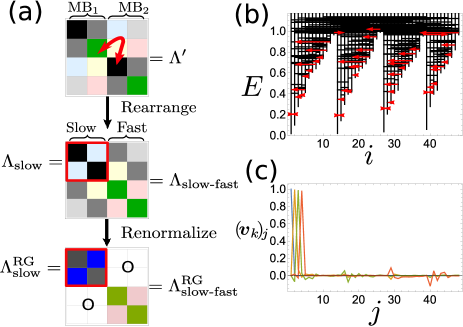
In the $K_{\sigma}$ representation, the intra-MB, diagonal blocks tend to be larger than the inter-MB, off-diagonal blocks, i.e., $\max_{i}\{K_{\sigma(\ell,i)\sigma(\ell,j)}\}>K_{\sigma(\ell^{\prime},i^{\prime})\sigma(\ell,j)}$ for arbitrary $\ell^{\prime}\neq\ell$ and $i^{\prime}$, since all LMs in a MB_ℓ are connected by most probable transitions. Hence, we regard the off-diagonal blocks as perturbations to the diagonal blocks. Thus, we first consider the block diagonal matrix $\text{diag}(K_{1},\dots,K_{\ell},\dots,K_{m})$, where $K_{\ell}$ is given by $(K_{\ell})_{ij}=k_{\sigma(\ell,i),\sigma(\ell,j)}-\delta_{ij}\sum^{n_{\ell}}_{{j^{\prime}=1}}k_{\sigma(\ell,j^{\prime}),\sigma(\ell,i)}$. Namely, $K_{\ell}$ describes the intra-MB_ℓ relaxations, whose $j$th eigenvalues $\lambda_{\ell,j}$ satisfy $0=\lambda_{\ell,0}>\lambda_{\ell,1}\geqslant\dots\geqslant\lambda_{\ell,n_{\ell}-1}$. The intra-MB relaxation modes are obtained as follows: By using the local equilibrium ${\bf\it p}_{\ell,0}$ in MB_ℓ satisfying $K_{\ell}{\bf\it p}_{\ell,0}=0$, we form $T_{\ell}=D_{\ell}^{-1}K_{\ell}D_{\ell}$, using the diagonal matrix $D_{\ell}$ with $(D_{\ell})_{i,i}=\sqrt{({\bf\it p}_{\ell,0})_{i}}$. $T_{\ell}$ is the symmetric matrix and can be diagonalized with an orthogonal matrix $S_{\ell}=\left[\sqrt{{\bf\it p}_{\ell,0}},{\bf\it v}_{\ell,1},\dots,{\bf\it v}_{\ell,n_{\ell}-1}\right]$, as $S_{\ell}^{T}T_{\ell}S_{\ell}=\text{diag}(0,\lambda_{\ell,1},\dots,\lambda_{\ell,n_{\ell}-1})\equiv\Lambda_{\ell}$, where the $j$th eigenvectors, ${\bf\it v}_{\ell,j}$, describe the $j$th intra-MB_ℓ relaxation modes of relaxation rates $\lambda_{\ell,j}$. Note here that $T_{\ell}$ is diagonalized more easily than the whole system of $K_{\sigma}$.

Next, we consider the inter-MB transitions. The global equilibrium ${\bf\it p}_{\text{eq}}$ satisfies $K_{\sigma}{\bf\it p}_{\text{eq}}=0$ as well as $\text{diag}(K_{1},K_{2},\dots){\bf\it p}_{\text{eq}}=0$. Hence, the diagonal matrix $D$ with $(D)_{i,i}=\sqrt{({\bf\it p}_{\text{eq}})_{i}}$ and $S=\text{diag}(S_{1},S_{2},\dots)$ satisfy $S^{T}D^{-1}\text{diag}(K_{1},K_{2},\dots)DS=\text{diag}(\Lambda_{1},\Lambda_{2},\dots)$. Hence, the symmetric matrix $\Lambda^{\prime}=S^{T}D^{-1}K_{\sigma}DS$ describes the couplings between intra-MB relaxation modes. Note that $\Lambda^{\prime}$ has nonzero off-diagonal elements not only in inter-MB off-diagonal blocks, but also in intra-MB diagonal blocks [Fig. 1(a), upper panel].

The unperturbed fast intra-MB relaxation modes promptly decay and would hardly contribute to the global slowest modes at all, while the unperturbed slow relaxation modes do interact with each other and mainly form the global slowest relaxation modes. Hence, we introduce a certain threshold $\lambda_{\text{cut}}$ and divide the unperturbed relaxation modes into two: the slow relaxation modes ($0\geqslant\lambda_{\ell,j}\geqslant\lambda_{\text{cut}}$) and the fast relaxation modes ($\lambda_{\text{cut}}>\lambda_{\ell,j}$) [Fig. 1(a), upper panel]. For the sake of convenience, we reorder the columns and lows of $\Lambda^{\prime}$ in the slow-to-fast relaxation block order, as shown in the middle panel of Fig. 1(a). The resultant matrix is denoted by $\Lambda_{\text{slow-fast}}$, where $\Lambda_{\text{slow}}$ is the first $n_{\text{slow}}\times n_{\text{slow}}$ submatrix with $n_{\text{slow}}$ denoting the number of unperturbed slow relaxation modes.

In the following, we first show that the existing coarse-graining procedures for kinetic problems, which assume intra-MB local equilibriums, are insufficient to obtain accurate results, as stated in BPE . Then, we develop a renormalization procedure with the use of the Jacobi method, where the resultant coarse-graining errors are reduced to zero.

Let us start with exemplifying how the coarse-graining procedure gives rise to errors with use of the four-funnel model depicted in Fig. 1(b). For simplicity, all frequency factors, $\nu_{ij}$, in the transition rate matrix are set to be $1$. With the use of the MB analysis, we obtain the following four MBs: $\text{MB}_{1}=\{\text{LM}_{1},\dots,\text{LM}_{12}\}$, $\text{MB}_{2}=\{\text{LM}_{13},\dots,\text{LM}_{26}\}$, $\text{MB}_{3}=\{\text{LM}_{27},\dots,\text{LM}_{37},\text{LM}_{48}\}$, and $\text{MB}_{4}=\{\text{LM}_{38},\dots,\text{LM}_{47}\}$. Here we set $\lambda_{\text{cut}}=0$ and the slow relaxation modes are thereby composed of four intra-MB local equilibria ($n_{\text{slow}}=4$). The corresponding $4\times 4$ submatrix $\Lambda_{\text{slow}}$ has the eigenvalues of $0,\ -0.104,\ -0.208$, and $-0.355$, which are approximations to the exact slowest four eigenvalues of $0,\ -0.089,\ -0.154$, and $-0.235$ at $\beta=5$. The discrepancies come from the inter-MB transitions. Figure 1(c) shows that the global relaxation modes are composed not only of slow unperturbed modes but also of fast relaxation modes. Namely, the couplings between slow and fast relaxation modes in $\Lambda_{\text{slow-fast}}$ also modify the couplings among the intra-MB slow modes. This is the reason why any existing coarse-graining procedures for kinetic problems, which simply neglect the fast intra-MB relaxation modes and assume the states to be linear combinations of intra-MB local equilibriums, are insufficient to obtain accurate results.

Now we construct a renormalized transition matrix, $\Lambda^{\text{RG}}_{\text{slow}}$, describing the global slowest relaxation modes accurately. To this end, we use a Jacobi rotation $\Lambda_{\text{slow-fast}}\mapsto\Lambda_{\text{slow-fast}}^{\text{RG}}=G^{T}\Lambda_{\text{slow-fast}}G$ such that the resultant couplings between slow and fast modes, $(\Lambda_{\text{slow-fast}}^{\text{RG}})_{ij}$ with $i\leqslant n_{\text{slow}}<j$, are vanishing. We here choose the repeated Givens matrix $G=G_{1}G_{2}\dots G_{r}$ for $G$, where $G_{s}=G(p_{s},q_{s},\theta_{s})$ are defined by $\left(G(p,q,\theta)\right)_{pp}=\left(G(p,q,\theta)\right)_{qq}=\cos\theta$, $\left(G(p,q,\theta)\right)_{pq}=-\left(G(p,q,\theta)\right)_{qp}=\sin\theta$, $\left(G(p,q,\theta)\right)_{ii}=1$ for $i\neq p,\ q$, otherwise $\left(G(p,q,\theta)\right)_{ij}=0$. In actual computation, we repeat the following procedures for $s=1,2,\dots,r$: We first choose $p_{s},q_{s}$ randomly from $p_{s}\leqslant n_{\text{slow}}<q_{s}$, and set $\theta_{s}$ as $\theta_{s}=\frac{1}{2}\tan^{-1}[{2(A_{s-1})_{p_{s}q_{s}}}/((A_{s-1})_{p_{s}p_{s}}-(A_{s-1})_{q_{s}q_{s}})]$, so as to eliminate $(p_{s},q_{s})$-entry of $A_{s}$, where $A_{s}=G_{s}^{T}\dots G_{1}^{T}\Lambda_{\text{slow-fast}}G_{1}\dots G_{s}$ and $A_{0}=\Lambda_{\text{slow-fast}}$. In short, this procedure is a Jacobi method, originally developed for symmetric matrix diagonalization matrixcomp , which is modified to eliminate not all the off-diagonal elements, but only those of the slow-fast couplings. Therefore, as the procedure is repeated sufficiently many times (say, $r$ times), the couplings between slow and fast relaxation modes in $A_{r}$ do converge to zero and these modes are decoupled in the final representation. Hence, we set $\Lambda_{\text{slow-fast}}^{\text{RG}}=A_{r}$ and $\Lambda^{\text{RG}}_{\text{slow}}$ is defined by the first $n_{\text{slow}}$-by-$n_{\text{slow}}$ submatrix of $\Lambda_{\text{slow-fast}}^{\text{RG}}$ [Fig. 1(a), lower panel]. It is $\Lambda^{\text{RG}}_{\text{slow}}$ that exactly describes the transitions among the renormalized slow relaxation modes.

Using the four-funnel model, we examined how the renormalization procedure works. First, we confirmed that the slow-fast coupling elements of $\Lambda^{\text{RG}}_{\text{slow-fast}}$ do converge to zero as in the lower panel of Fig. 1(a). The resultant matrices $\Lambda_{\text{slow}}$ and $\Lambda^{\text{RG}}_{\text{slow}}$ are as follows:

$$\Lambda_{\text{slow}} = \left(\begin{smallmatrix}-0.108&0.078&0.019&0.020\\ 0.078&-0.142&0.037&0.033\\ 0.019&0.037&-0.185&0.144\\ 0.020&0.033&0.144&-0.232\end{smallmatrix}\right),$$

$$\Lambda^{\text{RG}}_{\text{slow}} = \left(\begin{smallmatrix}-0.088&0.057&0.018&0.021\\ 0.057&-0.104&0.028&0.023\\ 0.018&0.028&-0.128&0.090\\ 0.021&0.023&0.090&-0.159\end{smallmatrix}\right).$$

Comparing these matrices, we see that the coupling terms between slow modes are modified by relative ratios of $0.01$–$0.1$, as a result of the renormalization. Due to the renormalization effect, we get the right eigenvalues of $0,\ -0.089,\ -0.154$, and $-0.235$ by diagonalizing $A^{\text{RG}}_{\text{slow}}$, which numerically agree with the above mentioned exact values of the slowest four eigenvalues at $\beta=5$.

Finally, the kinetics of vacancy diffusion in KCl nanoclusters niiyama is examined for a realistic problem. Suppose one chlorine ion is extracted from a cube of ionic crystal, with equal $N_{L}$-atom edges. Assume also that $N_{L}$ is an odd number $2n_{L}+1$ and the resultant (${N_{L}}^{3}-1$)-atom cluster is electrically neutral. Then, the vacancy moves around the cluster, which induces atomic diffusion. Note that the cubic form of the cluster is kept in the course of time evolution, when the temperature is sufficiently low cubic . At such low temperatures, the position of the vacancy is specified by the cubic lattice point $(n_{x},n_{y},n_{z})$ with $-n_{L}\leqslant n_{x},n_{y},n_{z}\leqslant n_{L}$. In addition, we are able to find the atomic structure of LM specified by $(n_{x},n_{y},n_{z})$ as follows: First, atoms are arranged at $d(m_{x},m_{y},m_{z})$ with lattice constant $d=3.147\ \text{\AA}$ for KCl, where $(m_{x},m_{y},m_{z})\neq(n_{x},n_{y},n_{z})$ and $-n_{L}\leqslant m_{x},m_{y},m_{z}\leqslant n_{L}$. Then, the configuration of atoms is relaxed to the LM energy structure by, e.g., steepest descent method. In this way, the LM atomic structure is assigned to $(n_{x},n_{y},n_{z})$. For computational details of enumerating LMs as well as SPs, we refer the reader to Ref. niiyama .

Figure 2: MBs of the $N_{L}=13$ cluster are represented by arrows (See text): (a) Eight MBs located at the vertexes, (b) Six MBs located at the faces, (c) 12 MBs located at the edges, and (d) 9 saddlelike MBs located in the central part. Thin red lines in (c) and thin black lines in (d) are drawn to show that the saddlelike MBs are hubs among the edge MBs.

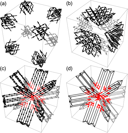
The MBs of the $N_{L}=13$ cluster at temperature $k_{\text{B}}T=0.03$ eV are depicted in Fig. 2, where the monotonic sequences, $\text{LM}_{i_{1}}\to\text{LM}_{i_{2}}\to\dots$, are shown by the arrows, $(n_{x},n_{y},n_{z})_{i_{1}}\to(n_{x},n_{y},n_{z})_{i_{2}}\to\dots$, which connect the corresponding vacancy lattice points. The collections of LMs with the same terminal LMs represent MBs. In Fig. 2(a), the eight most stable MBs, containing the lowest energy terminal LMs of $(\pm n_{L},\pm n_{L},\pm n_{L})$, are shown. In addition, there exist six MBs with terminal LMs at the centers of faces $(\pm n_{L},0,0)$, $(0,\pm n_{L},0)$, and $(0,0,\pm n_{L})$ [Fig. 2(b)], and 12 MBs with terminal LMs at the centers of edges $(\pm n_{L},\pm n_{L},0)$, $(\pm n_{L},0,\pm n_{L})$, and $(0,\pm n_{L},\pm n_{L})$ [Fig. 2(c)]. Moreover, due to the cubic symmetry, there are “saddlelike” LMs, which have at least two monotonic sequences reaching different terminal LMs. For example, eight monotonic sequences emanating from $(0,0,0)$ have terminal LMs at $(\pm n_{L},\pm n_{L},\pm n_{L})$. Hence, $(0,0,0)$ mediates the transitions among the vertex MBs like a saddle. To obtain a more coarse-grained description, we apply the MB analysis again only to saddlelike LMs and the SPs connecting these LMs endnote , to classify them into nine saddlelike MBs, as shown in Fig. 2(d).

We divide the intra-MB relaxation modes into slow and fast modes by setting $\lambda_{\text{cut}}=5.0\times 10^{5}\ \text{s}^{-1}$. The resultant total dimension of slow modes is $n_{\text{slow}}=137$. We first diagonalize the $137\times 137$ dimensional $\Lambda_{\text{slow}}$. The eigenvalues are plotted in Fig. 3(a), where the approximate result is in qualitative agreement with the exact result of $\Lambda_{\text{slow-fast}}$, although $n_{\text{slow}}=137$ is a quite small dimension compared to the full dimension of 1099. We then apply the renormalization procedure developed above to $\Lambda_{\text{slow-fast}}$, and obtain the renormalized $\Lambda^{\text{RG}}_{\text{slow}}$ and the Givens matrix $G$. After diagonalizing $\Lambda^{\text{RG}}_{\text{slow}}$, we also plot the eigenvalues of $\Lambda^{\text{RG}}_{\text{slow}}$ in Fig. 3(a), which shows that the slowest relaxations are exactly described by the quite small $137\times 137$ matrix of $\Lambda^{\text{RG}}_{\text{slow}}$.

Figure 3: (a) For the $N_{L}=13$ cluster at $k_{\text{B}}T=0.03$ eV, the slowest relaxation rates, $\lambda_{k}$ [$\times 10^{5}$s^-1], are plotted as a function of $k=0,1,\dots,17$. Markers ●, $\blacklozenge$, and $\blacksquare$ indicate the slowest eigenvalues of $\Lambda_{\text{slow}}$, $\Lambda_{\text{slow-fast}}$, and $\Lambda^{\text{RG}}_{\text{slow}}$, respectively. For the $k$th relaxation modes, $({\bf\it v}_{k})_{\ell}$ are plotted in (b) and (c). In the horizontal axes, $\ell=1,\dots,8$ (shaded) correspond to the vertex MBs, $\ell=9,\dots,14$ to the face-centered MBs, $\ell=15,\dots,26$ (shaded) to the edge-centered MBs, and $\ell=27,\dots,35$ to the saddlelike MBs. (b) Inter hetero-MB relaxation modes: ● and $\blacksquare$ are the results of $k=1$ and $11$, respectively, where $({\bf\it v}_{k})_{\ell}=({\bf\it v}_{k})_{\ell^{\prime}}$ hold for $\ell,\ell^{\prime}$ in the same type of MBs. In this case, the equilibrations occur only among the different types of MBs. (c) Inter iso-MB relaxation modes: ${\color[rgb]{0.368417,0.506779,0.709798}{\CIRCLE}}$, ${\color[rgb]{0.880722,0.611041,0.142051}{\blacksquare}}$, and ${\color[rgb]{0.560181,0.691569,0.194885}{\blacklozenge}}$ are, respectively, the results of $k=2$, 3, and 4, where $\sum_{\ell\in\text{same type of MBs}}({\bf\it v}_{k})_{\ell}\simeq 0$ hold. In this case, the equilibrations can occur only among the same type of MBs.

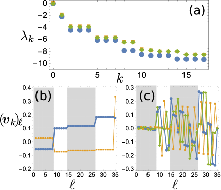
Now lastly, we show the usefulness of the metabasin representation for describing the slowest relaxation modes. We plot the intra-MB_ℓ equilibrium components, $({\bf\it v}_{k})_{\ell}$ of the $k$th slowest relaxation modes, ${\bf\it v}_{k}=G{\bf\it v}_{k}^{\text{RG}}$, in Figs. 3(b) and 3(c), from which we see that the global relaxations are grouped into two types: inter hetero-MB relaxation modes and inter iso-MB relaxation modes. As shown in Fig. 3(b), the inter hetero-MB modes equilibrate the disturbance only among different types of MBs. As a result, they equilibrate the disturbance along the radial direction from the cubic center. The plot for ${\bf\it v}_{1}$ in Fig. 3(b) shows that the bottleneck of equilibration is the process transporting the vacancy to the vertex MBs. On the other hand, the iso-MB equilibration modes equilibrate just among the same type of MBs, and moreover typically localize, as shown in Fig. 3(c). For example, as depicted in Fig. 3(c), the vertex MBs hardly equilibrate at all in these modes. To sum up, the slowest kinetics is two-step relaxation, the inter iso-MB relaxations of $\lambda_{2}$, $\lambda_{3}$, and $\lambda_{4}$, followed by the slowest inter hetero-MB relaxation of $\lambda_{1}$. It should be noted that these results were obtained with the use of the high accuracy renormalization procedure combined with the analysis by MB representation. Our method provides a firm and systematic basis for the elucidation in niiyama , where the bottleneck in the mixing process of the KCl cluster was numerically studied with the use of mean first passage times mfpt from the center LM to the vertex LMs.

In summary, we developed a renormalization procedure for transition rate matrices based on metabasin analysis, which is an accurate and efficient method for computing slowest relaxation modes. We also show, with the use of the multifunnel model and the ionic nanoparticle diffusion model, that the metabasin analysis is useful for grasping when, where, and how global equilibration occurs. Finally, it should be noted that this procedure can be extended to be applicable to transition probability matrices of discrete-time kinetic equations with small modifications sm . We hope that with these methods, characteristics of slowest relaxations are revealed for generic multi-metabasin systems.