Subspace Network: Deep Multi-Task Censored Regression for Modeling Neurodegenerative Diseases

Abstract.

Over the past decade a wide spectrum of machine learning models have been developed to model the neurodegenerative diseases, associating biomarkers, especially non-intrusive neuroimaging markers, with key clinical scores measuring the cognitive status of patients. Multi-task learning (MTL) has been commonly utilized by these studies to address high dimensionality and small cohort size challenges. However, most existing MTL approaches are based on linear models and suffer from two major limitations: 1) they cannot explicitly consider upper/lower bounds in these clinical scores; 2) they lack the capability to capture complicated non-linear interactions among the variables. In this paper, we propose Subspace Network, an efficient deep modeling approach for non-linear multi-task censored regression. Each layer of the subspace network performs a multi-task censored regression to improve upon the predictions from the last layer via sketching a low-dimensional subspace to perform knowledge transfer among learning tasks. Under mild assumptions, for each layer the parametric subspace can be recovered using only one pass of training data. Empirical results demonstrate that the proposed subspace network quickly picks up the correct parameter subspaces, and outperforms state-of-the-arts in predicting neurodegenerative clinical scores using information in brain imaging.

1. Introduction

Recent years have witnessed increasing interests on applying machine learning (ML) techniques to analyze biomedical data. Such data-driven approaches deliver promising performance improvements in many challenging predictive problems. For example, in the field of neurodegenerative diseases such as Alzheimer’s disease and Parkinson’s disease, researchers have exploited ML algorithms to predict the cognitive functionality of the patients from the brain imaging scans, e.g., using the magnetic resonance imaging (MRI) as in (Adeli-Mosabbeb et al., 2015; Zhang et al., 2012; Zhou et al., 2011b). A key finding points out that there are typically various types of prediction targets (e.g., cognitive scores), and they can be jointly learned using multi-task learning (MTL), e.g.,  (Caruana, 1998; Evgeniou and Pontil, 2004; Zhang et al., 2012), where the predictive information is shared and transferred among related models to reinforce their generalization performance.

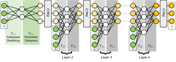
Figure 1. The proposed subspace network via hierarchical subspace sketching and refinement.

Two challenges persist despite the progress of applying MTL in disease modeling problems. First, it is important to notice that clinical targets, different from typical regression targets, are often naturally bounded. For example, in the output of Mini-Mental State Examination (MMSE) test, a key reference for deciding cognitive impairments, ranges from 0 to 30 (a healthy subject): a smaller score indicates a higher level of cognitive dysfunction (please refer to (Tombaugh and McIntyre, 1992)). Other cognitive scores, such as Clinical Dementia Rating Scale (CDR) (Hughes et al., 1982) and Alzheimer’s Disease Assessment Scale-Cog (ADAS- Cog) (Rosen et al., 1984), also have specific upper and lower bounds. Most existing approaches, e.g., (Zhang et al., 2012; Zhou et al., 2011b; Poulin et al., 2011), relied on linear regression without considering the range constraint, partially due to the fact that mainstream MTL models for regression, e.g., (Jalali et al., 2010; Argyriou et al., 2007; Zhang et al., 2012; Zhou et al., 2011a), are developed using the least squares loss and cannot be directly extended to censored regressions. As the second challenge, a majority of MTL research focused on linear models because of computational efficiency and theoretical guarantees. However, linear models cannot capture the complicated non-linear relationship between features and clinical targets. For example, (Association et al., 2013) showed the early onset of Alzheimer’s disease to be related to single-gene mutations on chromosomes 21, 14, and 1, and the effects of such mutations on the cognitive impairment are hardly linear (please refer to (Martins et al., 2005; Sweet et al., 2012)). Recent advances in multi-task deep neural networks (Seltzer and Droppo, 2013; Zhang et al., 2014; Wu et al., 2015) provide a promising direction, but their model complexity and demands of huge number of training samples prohibit their broader usages in clinical cohort studies.

To address the aforementioned challenges, we propose a novel and efficient deep modeling approach for non-linear multi-task censored regression, called Subspace Network (SN), highlighting the following multi-fold technical innovations:

• It efficiently builds up a deep network in a layer-by-layer feedforward fashion, and in each layer considers a censored regression problem. The layer-wise training allows us to grow a deep model efficiently.

• It explores a low-rank subspace structure that captures task relatedness for better predictions. A critical difference on subspace decoupling between previous studies such as (Mardani et al., 2015) (Shen et al., 2016) and our method lies on our assumption of a low-rank structure in the parameter space among tasks rather than the original feature space.

• By leveraging the recent advances in online subspace sensing (Mardani et al., 2015; Shen et al., 2016), we show that the parametric subspace can be recovered for each layer with feeding only one pass of the training data, which allows more efficient layer-wise training.

Synthetic experiments verify the technical claims of the proposed SN, and it outperforms various state-of-the-arts methods in modeling neurodegenerative diseases on real datasets.

2. Multi-task censored regression via parameter subspace sketching and refinement

In censored regression, we are given a set of $N$ observations $\mathcal{D}=\{(x_{i},y_{i})\}_{i=1}^{N}$ of $D$ dimensional feature vectors $\{x_{i}\in\mathbb{R}^{D}\}$ and $T$ corresponding outcomes $\{y_{i}\in\mathbb{R}^{T}_{+}\}$, where each outcome $y_{i,t}\in\mathbb{R}_{+}$, $t\in\{1,\cdots,T\}$, can be cognitive scores (e.g., MMSE and ADAS-Cog) or other biomarkers of interest such as proteomics. For each outcome, the censored regression assumes a nonlinear relationship between the features and the outcome through a rectified linear unit (ReLU) transformation, i.e., $y_{i,t}=\operatorname*{ReLU}\left(W_{t}^{\top}x_{i}+\epsilon\right)$ where $W_{t}\in\mathbb{R}^{D}$ is the coefficient for input features, $\epsilon$ is i.i.d. noise, and ReLU is defined by $\operatorname*{ReLU}(z)=\max(z,0)$. We can thus collectively represent the censored regression for multiple tasks by:

(1) $$y_{i}=\operatorname*{ReLU}\left(Wx_{i}+\epsilon\right),$$

where $W=[W_{1},\dots,W_{T}]^{\top}\in\mathbb{R}^{T\times D}$ is the coefficient matrix. We consider the regression problem for each outcome as a learning task. One commonly used task relationship assumption is that the transformation matrix $W\in\mathbb{R}^{T\times D}$ belongs to a linear low-rank subspace $\mathcal{U}$. The subspace allows us to represent $W$ as product of two matrices, $W=UV$, where columns of $U\in\mathbb{R}^{T\times R}=[U_{1},\dots,U_{T}]^{\top}$ span the linear subspace $\mathcal{U}$, and $V\in\mathbb{R}^{R\times D}$ is the embedding coefficient. We note that the output $y$ can be entry-wise decoupled, such that for each component $y_{i,t}=\operatorname*{ReLU}(U_{t}^{\top}Vx_{i}+\epsilon)$. By assuming Gaussian noise $\epsilon\sim\mathcal{N}(0,\sigma^{2})$, we derive the following likelihood function:

$$\Pr(y_{i,t},x_{i}|U_{t},V)=\phi\left(\frac{y_{i,t}-U_{t}^{\top}Vx_{i}}{\sigma}\right)\mathbb{I}(y_{i,t}\in(0,\infty))$$

$$+\left[1-Q\left(\frac{0-U_{t}^{\top}Vx_{i}}{\sigma}\right)\right]\mathbb{I}(y_{i,t}=0),$$

where $\phi$ is the probabilistic density function of the standardized Gaussian $N(0,1)$ and $Q$ is the standard Gaussian tail. $\sigma$ controls how accurately the low-rank subspace assumption can fit the data. Note that other noise models can be assumed here as well. The likelihood of $(x_{i},y_{i})$ pair is thus given by:

$$\Pr(y_{i},x_{i}|U,V)=\prod_{t=1}^{T}\bigg{\{}\phi\left(\frac{y_{i,t}-U_{t}^{\top}Vx_{i}}{\sigma}\right)\mathbb{I}(y_{i,t}\in(0,\infty))$$

$$+\left[1-Q\left(-\frac{U_{t}^{\top}Vx_{i}}{\sigma}\right)\right]\mathbb{I}(y_{i,t}=0)\bigg{\}}.$$

The likelihood function allows us to estimate subspace $U$ and coefficient $V$ from data $\mathcal{D}$. To enforce a low-rank subspace, one common approach is to impose a trace norm on $UV$, where trace norm of a matrix $A$ is defined by $\|A\|_{*}=\sum_{j}s_{j}(A)$ and $s_{j}(A)$ is the $j$th singular value of $A$. Since $\|UV\|_{*}=\min_{U,V}\frac{1}{2}(\|U\|_{F}^{2}+\|V\|_{F}^{2})$, e.g., see (Srebro et al., 2005; Mardani et al., 2015), the objective function of multi-task censored regression problem is given by:

(2) $$\min\nolimits_{U,V}-\sum\nolimits_{i=1}^{N}\log\Pr(y_{i},x_{i}|U,V)+\tfrac{\lambda}{2}(\|U\|_{F}^{2}+\|V\|_{F}^{2}).$$

2.1. An online algorithm

We propose to solve the objective in (2) via the block coordinate descent approach which is reduced to iteratively updating the following two subproblems:

(P:V) $$V^{+} =\operatorname*{arg\,min}\nolimits_{V}-\sum\nolimits_{i=1}^{N}\log\Pr(y_{i},x_{i}|U^{-},V)+\tfrac{\lambda}{2}\|V\|_{F}^{2},$$

(P:U) $$U^{+} =\operatorname*{arg\,min}\nolimits_{U}-\sum\nolimits_{i=1}^{N}\log\Pr(y_{i},x_{i}|U,V^{+})+\tfrac{\lambda}{2}\|U\|_{F}^{2}.$$

Define the instantaneous cost of the $i$-th datum:

$$g(x_{i},y_{i},U,V)=-\log\Pr(x_{i},y_{i}|U,V)+\tfrac{\lambda}{2}\|U\|_{F}^{2}+\tfrac{\lambda}{2}\|V\|_{F}^{2},$$

and the online optimization form of (2) can be recast as an empirical cost minimization given below:

$$\min\nolimits_{U,V}\tfrac{1}{N}\sum\nolimits_{i=1}^{N}g(x_{i},y_{i},U,V).$$

According to the analysis in Section 2.2, one pass of the training data can warrant the subspace learning problem. We outline the solver for each subproblem as follows:

Algorithm 1 Single-layer parameter subspace sketching and refinement.

Training data $\mathcal{D}=\{(x_{i},y_{i})\}_{i=1}^{N}$, rank parameters $\lambda$ and $R$,

parameter subspace $U$, parameter sketch $V$

Initialize $U^{-}$ at random

for $i=1,\dots,N$ do

     // 1. Sketching parameters in the current subspace

$$V^{+}=\operatorname*{arg\,min}\nolimits_{V}-\log\Pr(y_{i},x_{i}|U^{-},V)+\tfrac{\lambda}{2}\|V\|_{F}^{2}$$

     // 2. Parallel subspace refinement $\{U_{t}\}_{t=1}^{T}$

     for $t=1,\dots,T$ do

         $U_{t}^{+}=\operatorname*{arg\,min}\nolimits_{U_{t}}-\log\Pr(y_{i,t},x_{i}|U_{t},V^{+})+\frac{\lambda}{2}\|U_{t}\|_{2}^{2}$

     end for

     Set $U^{-}=U^{+},V^{-}=V^{+}$

end for

Problem (P:V) sketches parameters in the current space. We solve (P:V) using gradient descent. The parameter sketching couples all the subspace dimensions in $V$ (not decoupled as in (Shen et al., 2016)), and thus we need to solve this collectively. The update of $V$ ($V^{+}$) can be obtained by solving the online problem given below:

$$\min_{V}g(x_{i},y_{i};U^{-},V)\equiv-\sum\nolimits_{t=1}^{T}\log\Pr(y_{i,t},x|U^{-}_{t},V)+\frac{\lambda}{2}\|V\|_{F}^{2}$$

$$=-\sum_{t=1}^{T}\log\bigg{[}\phi\left(\frac{y_{i,t}-\left(U_{t}^{-}\right)^{\top}Vx}{\sigma}\right)\mathbb{I}(y_{i,t}\in(0,\infty))$$

$$+\left[1-Q\left(\frac{-\left(U_{t}^{-}\right)^{\top}Vx}{\sigma}\right)\right]\mathbb{I}(y_{i,t}=0)\bigg{]}+\frac{\lambda}{2}\|V\|_{F}^{2}.$$

$V^{+}$ can be computed by the following gradient update: $V^{+}=V^{-}-\eta\nabla_{V}g(x_{i},y_{i};U^{-},V^{+}),$ where the gradient is given by:

$$\nabla_{V} g(x_{i},y_{i};U^{-},V^{+})=\lambda V+\sum_{t=1}^{T}\begin{cases}-\frac{y_{i,t}-\left(U^{-}_{t}\right)^{\top}Vx_{i}}{\sigma^{2}}U^{-}_{t}x_{i}^{\top}&y_{i,t}\in(0,\infty)\\ \frac{\phi(z_{t})}{\sigma\left[1-Q(z_{i,t})\right]}U^{-}_{t}x_{i}^{T}&y_{i,t}=0\end{cases}$$

where $z_{i,t}=\sigma^{-1}(-\left(U_{t}^{-}\right)^{\top}Vx)$. The algorithm for solving (P:V) is summarized in Alg. 2.

Algorithm 2 Gradient descent algorithm for problem P:V.

Training data $(x_{i},y_{i})$, $U^{-}$, step size $\eta$,

sketch $V$

Initialize $V^{-}$ at random.

// 1. Perform gradient step and update the current solution of V.

for $t=1,\dots,T$ do

     Compute $z_{i,t}=\sigma^{-1}(-\left(U_{t}^{-}\right)^{\top}Vx_{i})$.

     Compute the gradient for $y_{t}$:

$$\nabla{g}_{t} (x_{i},y_{i,t};U^{-},V^{+})=\begin{cases}-\frac{y_{i,t}-\left(U^{-}_{t}\right)^{\top}Vx_{i}}{\sigma^{2}}U^{-}_{t}x_{i}^{\top}&y_{i,t}\in(0,\infty)\\ \frac{\phi(z_{i,t})}{\sigma\left[1-Q(z_{i,t})\right]}U^{-}_{t}x_{i}^{\top}&y_{i,t}=0\end{cases}$$

end for

// 2. Update the current sketch $V^{-}$

$$V^{+}=V^{-}-\eta\left[\sum\nolimits_{t=1}^{T}\nabla{g}_{t}(x,y_{t};U^{-},V^{+})+\lambda V\right]$$

Set $V^{-}=V^{+}$

Problem (P:U) refines the subspace $U^{+}$ based on sketching. We solve (P:U) using stochastic gradient descent (SGD). We note that the problem is decoupled for different subspace dimensions $t=1,\dots,T$ (i.e., rows of $U$). With careful parallel design, this procedure can be done very efficiently. Given a training data point $(x_{i},y_{i})$, the problem related to the $t$-th subspace basis is:

$$\min_{U_{t}}g_{t}(x_{i},y_{i,t};U_{t},V^{+})\equiv-\log\Pr(y_{i,t},x_{i}|U_{t},V^{+})+\frac{\lambda}{2}\|U_{t}\|_{2}^{2}$$

$$=-\log\bigg{[}\phi\left(\frac{y_{i,t}-U_{t}^{\top}V^{+}x_{i}}{\sigma}\right)\mathbb{I}(y_{i,t}\in(0,\infty))$$

$$+\left[1-Q\left(\frac{-U_{t}^{\top}V^{+}x_{i}}{\sigma}\right)\right]\mathbb{I}(y_{i,t}=0)\bigg{]}+\frac{\lambda}{2}\|U_{t}\|_{2}^{2}.$$

We can revise subspace by the following gradient update: $U_{t}^{+}=U_{t}^{-}-\mu_{t}\nabla_{U_{t}}g_{t}(x_{i},y_{i,t};U_{t},V^{+}),$ where the gradient is given by:

$$\nabla_{U_{t}} g_{t}(x_{i},y_{i,t};U_{i,t},V^{+})=\lambda U_{t}+\begin{cases}-\frac{y_{i,t}-U_{t}^{\top}V^{+}x}{\sigma^{2}}V^{+}x_{i}&y_{i,t}\in(0,\infty)\\ \frac{\phi(z_{i,t})}{\sigma\left[1-Q(z_{i,t})\right]}V^{+}x_{i}&y_{i,t}=0\end{cases}$$

where $z_{i,t}=\sigma^{-1}(-U_{t}^{\top}V^{+}x_{i})$. We summarize the procedure in Algorithm 1 and show in Section 2.2 that under mild assumptions this procedure will be able to capture the underlying subspace structure in the parameter space with just one pass of the data.

2.2. Theoretical results

We establish both asymptotic and non-asymptotic convergence properties for Algorithm 1. The proof scheme is inspired by a series of previous works: (Mairal et al., 2010; Kasiviswanathan et al., 2012; Shalev-Shwartz et al., 2012; Mardani et al., 2013, 2015; Shen et al., 2016). We briefly present the proof sketch, and more proof details can be found in Appendix. At each iteration $i=1,2,...,N$, we sample $(x_{i},y_{i})$, and let $U^{i},V^{i}$ denote the intermediate $U$ and $V$, to be differentiated from $U_{t},V_{t}$ which are the $t$-th columns of $U,V$. For the proof feasibility, we assume that $\{(x_{i},y_{i})\}_{i=1}^{N}$ are sampled i.i.d., and the subspace sequence $\{U^{i}\}_{i=1}^{N}$ lies in a compact set.

Asymptotic Case: To estimate $U$, the Stochastic Gradient Descent (SGD) iterations can be seen as minimizing the approximate cost $\frac{1}{N}\sum_{i=1}^{N}g^{\prime}(x_{i},y_{i},U,V)$, where $g^{\prime}$ is a tight quadratic surrogate for $g$ based on the second-order Taylor approximation around $U^{N-1}$. Furthermore, $g$ can be shown to be smooth, by bounding its first-order and second-order gradients w.r.t. each $U_{t}$ (similar to Appendix 1 of (Shen et al., 2016)).

Following (Mairal et al., 2010; Mardani et al., 2015), it can then be established that, as $N\rightarrow\infty$, the subspace sequence $\{U^{i}\}_{i=1}^{N}$ asymptotically converges to a stationary-point of the batch estimator, under a few mild conditions. We can sequentially show: 1) $\sum_{i=1}^{N}g^{\prime}(x_{i},y_{i},U^{i},V^{i})$ asymptotically converges to $\sum_{i=1}^{N}g(x_{i},y_{i},U^{i},V^{i})$, according to the quasi-martingale property in the almost sure sense, owing to the tightness of $g^{\prime}$; 2) the first point implies convergence of the associated gradient sequence, due to the regularity of $g$; 3) $g_{t}(x_{i},y_{i},U,V)$ is bi-convex for block variables $U_{t}$ and $V$.

Non-Asymptotic Case: When $N$ is finite, (Mardani et al., 2013) asserts that the distance between successive subspace estimates will vanish as fast as $O(1/i)$: $\|U^{i}-U^{i-1}\|_{F}\leq\frac{B}{i}$, for some constant $B$ that is independent of $i$ and $N$. Following (Shen et al., 2016) to leverage the unsupervised formulation of regret analysis as in (Kasiviswanathan et al., 2012; Shalev-Shwartz et al., 2012), we can similarly obtain a tight regret bound that will again vanish if $N\rightarrow\infty$.

3. Subspace network via hierarchical sketching and refinement

Algorithm 3 Network expansion via hierarchical parameter subspace sketching and refinement.

Training data $\mathcal{D}=\{(x_{i},y_{i})\}$, target network depth $K$.

The deep subspace network $f$

Set $f_{[0]}(x)=y$ and solve $f_{[0]}$ using Algorithm 1.

for $k=1,\dots,K-1$ do

     // 1. Subspace sketching based on the current subspace using Algorithm 1:

$$U_{[k]}^{*},V_{[k]}^{*}=\operatorname*{arg\,min}\limits_{U_{[k]},V_{[k]}}\mathbb{E}_{(x,y)\sim\mathcal{D}}\left\{\ell(y,\operatorname*{ReLU}\left(U_{[k]}V_{[k]}f_{[k-1]}(x)\right))\right\},$$

     // 2. Expand the layer using the refined subspace as our new network:

$$f_{[k]}(x)=\operatorname*{ReLU}\left(U_{[k]}^{*}V_{[k]}^{*}f_{[k-1]}(x)\right)$$

end for

return $f=f_{[K]}$

The single layer model in (1) has limited capability to capture the highly nonlinear regression relationships, as the parameters are linearly linked to the subspace except for a ReLU operation. However, the single-layer procedure in Algorithm 1 has provided a building block, based on which we can develop an efficient algorithm to train a deep subspace network (SN) in a greedy fashion. We thus propose a network expansion procedure to overcome such limitation.

After we obtain the parameter subspace $U$ and sketch $V$ for the single-layer case (1), we project the data points by $\bar{x}=\operatorname*{ReLU}(UVx)$. A straightforward idea of the expansion is to use $(\bar{x},y)$ as the new samples to train another layer. Let $f_{[k-1]}$ denote the network structure we obtained before the $k$-th expansion starts, $k=1,2,...,K-1$, the expansion can recursively stack more ReLU layers:

(3) $$f_{[k]}(x)=\operatorname*{ReLU}\left(U_{[k]}V_{[k]}f_{[k-1]}(x)+\epsilon\right),$$

However, we observe that simply stacking layers by repeating (3) many times can cause substantial information loss and degrade the generalization performance, especially since our training is layer-by-layer without “looking back” (i.e., top-down joint tuning). Inspired by deep residual networks (He et al., 2016) that exploit “skip connections” to pass lower-level data and features to higher levels, we concatenate the original samples with the newly transformed, censored outputs after each time of expansion, i.e., reformulating $\bar{x}=[\operatorname*{ReLU}(UVx);x]$ (similar manners could be found in (Zhou and Feng, 2017)). The new formulation after the expansion is given below:

$$f_{[k]}(x)=\operatorname*{ReLU}\left(U_{[k]}V_{[k]}\left[f_{[k-1]}(x);x\right]+\epsilon\right).\vspace{-1em}$$

We summarize the network expansion process in Alg. 3. The architecture of the resulting SN is illustrated in Fig. 1. Compared to the single layer model (1), SN gradually refines the parameter subspaces by multiple stacked nonlinear projections. It is expected to achieve superior performance due to the higher learning capacity, and the proposed SN can also be viewed as a gradient boosting method. Meanwhile, the layer-wise low-rank subspace structural prior would further improve generalization compared to naive multi-layer networks.

4. Experiment

The subspace network code and scripts for generating the results in this section are available at https://github.com/illidanlab/subspace-net.

4.1. Simulations on Synthetic Data

Subspace recovery in a single layer model. We first evaluate the subspace recovered by the proposed Algorithm 1 using synthetic data. We generated $X\in\mathbb{R}^{N\times D}$, $U\in\mathbb{R}^{T\times R}$ and $V\in\mathbb{R}^{R\times D}$, all as i.i.d. random Gaussian matrices. The target matrix $Y\in\mathbb{R}^{N\times T}$ was then synthesized using (1). We set $N=5,000$, $D=200$, $T=100$ $R=10$, and random noise as $\epsilon\sim\mathcal{N}(0,3^{2})$.

Figure 2a shows the plot of subspace difference between the ground-truth $U$ and the learned subspace $U_{i}$ throughout the iterations, i.e., $\|U-U_{i}\|_{F}/\|U\|_{F}$ w.r.t. $i$. This result verifies that Algorithm 1 is able to correctly find and smoothly converge to the underlying low-rank subspace of the synthetic data. The objective values throughout the online training process of Algorithm 1 are plotted in Figure 2b. We further show the plot of iteration-wise subspace differences, defined as $\|U_{i}-U_{i-1}\|_{F}/\|U\|_{F}$, in Figure 2c, which complies with the $o(1/t)$ result in our non-asymptotic analysis. Moreover, the distribution of correlation between recovered weights and true weights for all tasks is given in Figure 3, with most predicted weights having correlations with ground truth of above 0.9.

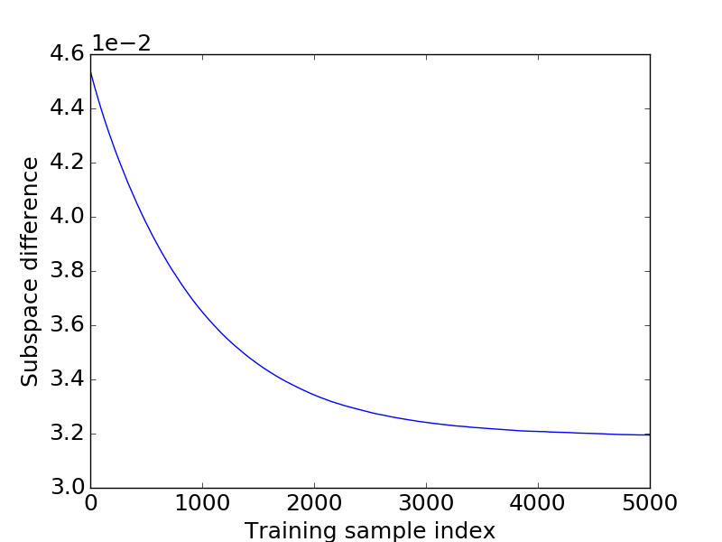
(a)

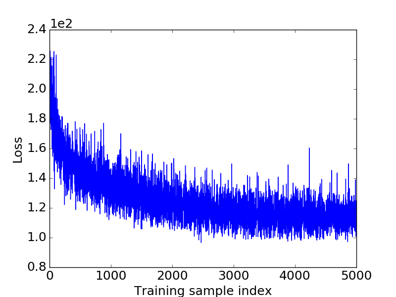
(b)

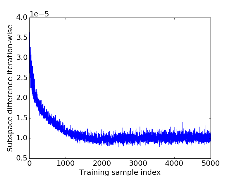
(c)

Figure 2. Experimental results on subspace convergence. (a) Subspace differences, w.r.t. the index $i$; (b) Convergence of Algorithm 1, w.r.t. the index $i$; (c) Iteration-wise subspace differences, w.r.t. the index $i$.

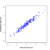
(a)

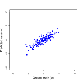
(b)

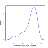
(c)

Figure 3. (a) Predicted weight vs true weight for task 1; (b) Predicted weight vs true weight for task 2; (c) Distribution of correlation between predicted weight and true weight for all tasks

Table 1. Comparison of subspace differences for each layer of SN, f-MLP, and rf-MLP.

Metric	Subspace Difference			Maximum Mutual Coherence			Mean Mutual Coherence
Method	SN	f-MLP	rf-MLP	SN	f-MLP	rf-MLP	SN	f-MLP	rf-MLP
Layer 1	0.0313	0.0315	0.0317	0.7608	0.7727	0.7895	0.2900	0.2725	0.2735
Layer 2	0.0321	0.0321	0.0321	0.8283	0.7603	0.7654	0.2882	0.2820	0.2829
Layer 3	0.0312	0.0315	0.0313	0.8493	0.7233	0.7890	0.2586	0.2506	0.2485

Subspace recovery in a multi-layer subspace network. We re-generated synthetic data by repeatedly applying (1) for three times, each time following the same setting as the single-layer model. A three-layer SN was then learned using Algorithm 3. As one simple baseline, a multi-layer perceptron (MLP) is trained, whose three hidden layers have the same dimensions as the three ReLU layers of the SN. Inspired by (Xue et al., 2013; Sainath et al., 2013; Wang et al., 2015), we then applied low-rank matrix factorization to each layer of MLP, with the same desired rank $R$, creating the factorized MLP (f-MLP) baseline that has the identical architecture (including both ReLU hidden layers and linear bottleneck layers) to SN. We further re-trained the f-MLP on the same data from end to end, leading to another baseline, named retrained factorized MLP (rf-MLP).

Table 1 evaluates the subspace recovery fidelity in three layers, using three different metrics: (1) the maximum mutual coherence of all column pairs from two matrices, defined in (Candes and Romberg, 2007) as a classical measurement on how correlated the two matrices’ column subspaces are; (2) the mean mutual coherence of all column pairs from two matrices; (3) the subspace difference defined the same as in the single-layer case. Note that the two mutual coherence-based metrics are immune to linear transformations of subspace coordinates, to which the $\ell_{2}$-based subspace difference might become fragile. SN achieves clear overall advantages under all three measurements, over f-MLP and rf-MLP. More notably, while the performance margin of SN in subspace difference seems to be small, the much sharper margins, in two (more robust) mutual coherence-based measurements, suggest that the recovered subspaces by SN are significantly better aligned with the groundtruth.

Table 2. Average normalized mean square error under different approaches for synthetic data.

Percent	Single Task (Shallow)			Multi Task (Shallow)
	Uncensored (LS + $\ell_{1}$)	Censored (LS + $\ell_{1}$)	Nonlinear Censored (Tobit)	Uncensored (Multi Trace)	Censored (Multi Trace)
40%	0.1412 (0.0007)	0.1127 (0.0010)	0.0428 (0.0003)	0.1333 (0.0009)	0.1053 (0.0027)
50%	0.1384 (0.0005)	0.1102 (0.0010)	0.0408 (0.0004)	0.1323 (0.0010)	0.1054 (0.0042)
60%	0.1365 (0.0005)	0.1088 (0.0009)	0.0395 (0.0003)	0.1325 (0.0012)	0.1031 (0.0046)
70%	0.1349 (0.0005)	0.1078 (0.0010)	0.0388 (0.0004)	0.1315 (0.0013)	0.1024 (0.0042)
80%	0.1343 (0.0011)	0.1070 (0.0012)	0.0383 (0.0006)	0.1308 (0.0008)	0.1040 (0.0011)
Percent	Deep Neural Network			Subspace Net (SN)
	DNN i (naive)	DNN ii (censored)	DNN iii (censored + low-rank)	Layer 1	Layer 3
40%	0.0623 (0.0041)	0.0489 (0.0035)	0.0431 (0.0041)	0.0390 (0.0004)	0.0369 (0.0002)
50%	0.0593 (0.0048)	0.0462 (0.0042)	0.0400 (0.0039)	0.0389 (0.0007)	0.0366 (0.0003)
60%	0.0587 (0.0053)	0.0455 (0.0054)	0.0395 (0.0050)	0.0388 (0.0006)	0.0364 (0.0003)
70%	0.0590 (0.0071)	0.0447 (0.0043)	0.0386 (0.0058)	0.0388 (0.0006)	0.0363 (0.0003)
80%	0.0555 (0.0057)	0.0431 (0.0053)	0.0380 (0.0057)	0.0390 (0.0008)	0.0364 (0.0005)

Table 3. Average normalized mean square error at each layer for subspace network ($R=10$) for synthetic data.

Perc.	Layer 1	Layer 2	Layer 3	Layer 10	Layer 20
40%	0.0390 (0.0004)	0.0381 (0.0005)	0.0369 (0.0002)	0.0368 (0.0002)	0.0368 (0.0002)
50%	0.0389 (0.0007)	0.0379 (0.0005)	0.0366 (0.0003)	0.0366 (0.0003)	0.0365 (0.0003)
60%	0.0388 (0.0006)	0.0378 (0.0004)	0.0364 (0.0003)	0.0364 (0.0003)	0.0363 (0.0003)
70%	0.0388 (0.0006)	0.0378 (0.0005)	0.0363 (0.0003)	0.0363 (0.0003)	0.0362 (0.0003)
80%	0.0390 (0.0008)	0.0378 (0.0006)	0.0364 (0.0005)	0.0363 (0.0005)	0.0363 (0.0005)

Benefits of Going Deep. We re-generate synthetic data again in the same way as the first single-layer experiment; yet differently, we now aim to show that a deep SN will boost performance over single-layer subspace recovery, even the data generation does not follow a known multi-layer model. We compare SN (both 1-layer and 3-layer) with two carefully chosen sets of state-of-art approaches: (1) single and multi-task “shallow” models; (2) deep models. For the first set, the least squares (LS) is treated as a naive baseline, while ridge (LS + $\ell_{2}$) and lasso (LS + $\ell_{1}$) regressions are considered for shrinkage or variables selection purpose; Censor regression, also known as the Tobit model, is a non-linear method to predict bounded targets , e.g., (Berberidis et al., 2016). Multi-task models with regularizations on trace norm (Multi Trace) and $\ell_{2,1}$ norm (Multi $\ell_{2,1}$) have been demonstrated to be successful on simultaneous structured/sparse learning, e.g., (Yang et al., 2010; Zhang et al., 2013). We also verify the benefits of accounting for boundedness of targets (Uncensored vs. Censored) in both single-task and multi-task settings, with best performance reported for each scenario (LS + $\ell_{1}$ for single-task and Multi Trace for multi-task). For the set of deep model baselines, we construct three DNNs for fair comparison: i) A 3-layer fully connected DNN with the same architecture as SN, with a plain MSE loss; ii) A 3-layer fully connected DNN as i) with ReLU added for output layer before feeding into the MSE loss, which naturally implements non-negativity censored training and evaluation; iii) A factorized and re-trained DNN from ii), following the same procedure of rf-MLP in the multi-layer synthetic experiment. Apparently, ii) and iii) are constructed to verify if DNN also benefits from the censored target and the low-rank assumption, respectively.

We performed 10-fold random-sampling validation on the same dataset, i.e., randomly splitting into training and validation data 10 times. For each split, we fitted model on training data and evaluated the performance on validation data. Average normalized mean square error (ANMSE) across all tasks was obtained as the overall performance for each split. For methods without hyper parameters (least square and censor regression), an average of ANMSE for 10 splits was regarded as the final performance; for methods with tunable parameters, e.g., $\lambda$ in lasso, we performed a grid search on $\lambda$ values and chose the optimal ANMSE result. We considered different splitting sizes with training samples containing [40%, 50%, 60%, 70%, 80%] of all the samples.

Table 2 further compares the performance of all approaches. Standard deviation of 10 trials is given in parenthesis (same for all following tables). We can observe that: (1) all censored models significantly outperform their uncensored counterparts, verifying the necessity of adding censoring targets for regression. Therefore, we will use censored baselines hereinafter, unless otherwise specified; (2) the more structured MTL models tend to outperform single task models by capturing task relatedness. That is also evidenced by the performance margin of DNN iii over DNN i; (3) the nonlinear models are undoubtedly more favorable: we even see the single-task Tobit model to outperform MTL models; (4) As a nonlinear, censored MTL model, SN combines the best of them all, accounting for its superior performance over all competitors. In particular, even a 1-layer SN already produces comparable performance to the 3-layer DNN iii (which also a nonlinear, censored MTL model trained with back-propagation, with three times the parameter amount of SN), thanks to SN’s theoretically solid online algorithm in sketching subspaces.

Furthermore, increasing the number of layers in SN from 2 to 20 demonstrated that SN can also benefit from growing depth without an end to end scheme. As Table 3 reveals, SN steadily improves with more layers, until reaching a plateau at $\sim 5$ layers (as the underlying data distribution is relatively simple here). The observation is consistent among all splits.

Computation speed. All experiments run on the same machine (1 x Six-core Intel Xeon E5-1650 v3 [3.50GHz], 12 logic cores, 128 GB RAM). GPU accelerations are enabled for DNN baselines, while SN has not exploited the same accelerations yet. The running time for a single round training on synthetic data (N=5000, D=200, T=100) is given in Table 4. Training each layer of SN will cost 109 seconds on average. As we can see, SN improves generalization performance without a significant computation time burden. Furthermore, we can accelerate SN further, by reading data in batch mode and performing parallel updates.

Table 4. Running time on synthetic data.

Method	Time (s)	Platform
Least Square	0.02	Matlab
LS+$\ell_{2}$	0.02	Matlab
LS+$\ell_{1}$	18.4	Matlab
Multi-trace	32.3	Matlab
Multi-$\ell_{21}$	27.0	Matlab
Censor	1680	Matlab
SN (per layer)	109	Python
DNN	659	Tensorflow

Table 5. Average normalized mean square error at each layer for subspace network ($R=5$) for real data.

Percent	Layer 1	Layer 2	Layer 3	Layer 5	Layer 10
40%	0.2016 (0.0057)	0.2000 (0.0039)	0.1981 (0.0031)	0.1977 (0.0031)	0.1977 (0.0031)
50%	0.1992 (0.0040)	0.1992 (0.0053)	0.1971 (0.0038)	0.1968 (0.0036)	0.1967 (0.0035)
60%	0.1990 (0.0061)	0.1990 (0.0047)	0.1967 (0.0038)	0.1964 (0.0039)	0.1964 (0.0038)
70%	0.1981 (0.0046)	0.1966 (0.0052)	0.1953 (0.0039)	0.1952 (0.0039)	0.1951 (0.0038)
80%	0.1970 (0.0034)	0.1967 (0.0044)	0.1956 (0.0040)	0.1955 (0.0039)	0.1953 (0.0039)

Table 6. Average normalized mean square error under different approaches for real data.

Percent	Single Task (Censored)			Multi Task (Censored)
	Least Square	LS + $\ell_{1}$	Tobit (Nonlinear)	Multi Trace	Multi $\ell_{2,1}$
40%	0.3874 (0.0203)	0.2393 (0.0056)	0.3870 (0.0306)	0.2572 (0.0156)	0.2006 (0.0099)
50%	0.3119 (0.0124)	0.2202 (0.0049)	0.3072 (0.0144)	0.2406 (0.0175)	0.2002 (0.0132)
60%	0.2779 (0.0123)	0.2112 (0.0055)	0.2719 (0.0114)	0.2596 (0.0233)	0.2072 (0.0204)
70%	0.2563 (0.0108)	0.2037 (0.0042)	0.2516 (0.0108)	0.2368 (0.0362)	0.2017 (0.0116)
80%	0.2422 (0.0112)	0.2005 (0.0054)	0.2384 (0.0099)	0.2176 (0.0171)	0.2009 (0.0050)
Percent	Deep Neural Network			Subspace Net (SN)
	DNN i (naive)	DNN ii (censored)	DNN iii (censored + low-rank)	Layer 1	Layer 3
40%	0.2549 (0.0442)	0.2388 (0.0121)	0.2113 (0.0063)	0.2016 (0.0057)	0.1981 (0.0031)
50%	0.2236 (0.0066)	0.2208 (0.0062)	0.2127 (0.0118)	0.1992 (0.0040)	0.1971 (0.0038)
60%	0.2215 (0.0076)	0.2200 (0.0076)	0.2087 (0.0102)	0.1990 (0.0061)	0.1967 (0.0038)
70%	0.2149 (0.0077)	0.2141 (0.0079)	0.2093 (0.0137)	0.1981 (0.0046)	0.1953 (0.0039)
80%	0.2132 (0.0138)	0.2090 (0.0079)	0.2069 (0.0135)	0.1970 (0.0034)	0.1956 (0.0040)

Table 7. Average normalized mean square error under different rank assumptions for real data.

Method	Percent - Rank	$R=1$	$R=3$	$R=5$	$R=10$
SN	40%	0.2052 (0.0030)	0.1993 (0.0036)	0.1981 (0.0031)	0.2010 (0.0044)
	50%	0.2047 (0.0029)	0.1983 (0.0034)	0.1971 (0.0038)	0.2001 (0.0046)
	60%	0.2052 (0.0033)	0.1988 (0.0047)	0.1967 (0.0038)	0.1996 (0.0052)
	70%	0.2043 (0.0044)	0.1975 (0.0042)	0.1953 (0.0039)	0.1990 (0.0057)
	80%	0.2058 (0.0051)	0.1977 (0.0042)	0.1956 (0.0040)	0.1990 (0.0058)
DNN iii (censored + low-rank)	40%	0.2322 (0.0146)	0.2360 (0.0060)	0.2113 (0.0063)	0.2196 (0.0124)
	50%	0.2298 (0.0093)	0.2256 (0.0127)	0.2127 (0.0118)	0.2235 (0.0142)
	60%	0.2244 (0.0132)	0.2277 (0.0099)	0.2087 (0.0102)	0.2145 (0.0208)
	70%	0.2178 (0.0129)	0.2177 (0.0115)	0.2093 (0.0137)	0.2083 (0.0127)
	80%	0.2256 (0.0117)	0.2250 (0.0079)	0.2069 (0.0135)	0.2158 (0.0183)

Table 8. Average normalized mean square error for non-calibrated vs. calibrated SN for real data (6 layers).

Percent	Non-calibrate	Calibrate
40%	0.1993 (0.0034)	0.1977 (0.0031)
50%	0.1987 (0.0043)	0.1967 (0.0036)
60%	0.1991 (0.0044)	0.1964 (0.0039)
70%	0.1982 (0.0042)	0.1951 (0.0038)
80%	0.1984 (0.0041)	0.1954 (0.0039)

4.2. Experiments on Real data

We evaluated SN in a real clinical setting to build models for the prediction of important clinical scores representing a subject’s cognitive status and signaling the progression of Alzheimer’s disease (AD), from structural Magnetic Resonance Imaging (sMRI) data. AD is one major neurodegenerative disease that accounts for 60 to 80 percent of dementia. The National Institutes of Health has thus focused on studies investigating brain and fluid biomarkes of the disease, and supported the long running project Alzheimer’s Disease Neuroimaging Initiative (ADNI) from 2003. We used the ADNI-1 cohort (http://adni.loni.usc.edu/). In the experiments, we used the 1.5 Tesla structural MRI collected at the baseline, and performed cortical reconstruction and volumetric segmentations with the FreeSurfer following the procotol in (Jack et al., 2008). For each MRI image, we extracted 138 features representing the cortical thickness and surface areas of region-of-interests (ROIs) using the Desikan-Killiany cortical atlas (Desikan et al., 2006). After preprocessing, we obtained a dataset containing 670 samples and 138 features. These imaging features were used to predict a set of 30 clinical scores including ADAS scores (Rosen et al., 1984) at baseline and future (6 months from baseline), baseline Logical Memory from Wechsler Memory Scale IV (Scale—Fourth, 2009), Neurobattery scores (i.e. immediate recall total score and Rey Auditory Verbal Learning Test scores), and the Neuropsychiatric Inventory (Cummings, 1997) at baseline and future.

Calibration. In MTL formulations we typically assume that noise variance $\sigma^{2}$ is the same across all tasks, which may not be true in many cases. To deal with heterogeneous $\sigma^{2}$ among tasks, we design a calibration step in our optimization process, where we estimate task-specific $\hat{\sigma}_{t}^{2}$ using $\|y-\hat{y}\|_{2}^{2}/N$ before ReLU, as the input for next layer and repeat on layer-wise. We compare performance of both non-calibrated and calibrated methods.

Performance. We adopted the two sets of baselines used in the last synthetic experiment for the real world data. Different from synthetic data where the low-rank structure was predefined, for real data, there is no groundtruth rank available and we have to try different rank assumptions. Table 8 compares the performances between $\sigma^{2}$ non-calibrated versus calibrated models. We observe a clear improvement by assuming different $\sigma^{2}$ across tasks. Table 6 shows the results for all comparison methods, with SN outperforming all else. Table 5 shows the SN performance growth with increasing the number of layers. Table 7 further reveals the performance of DNNs and SN using varying rank estimations in real data. As expected, the U-shape curve suggests that an overly low rank may not be informative enough to recover the original weight space, while a high-rank structure cannot enforce as strong a structural prior. However, the overall robustness of SN to rank assumptions is fairly remarkable: its performance under all ranks is competitive, consistently outperforming DNNs under the same rank assumptions and other baselines.

Qualitative Assessment. From the multi-task learning perspective, the subspaces serve as the shared component for transferring predictive knowledge among the censored learning tasks. The subspaces thus capture important predictive information in predicting cognitive changes. We normalized the magnitude of the subspace into the range of $[-1,1]$ and visualized the subspace in brain mappings. The the 5 lowest level subspaces in $V_{1}$ are the most important five subspaces, and is illustrated in Figure 4.

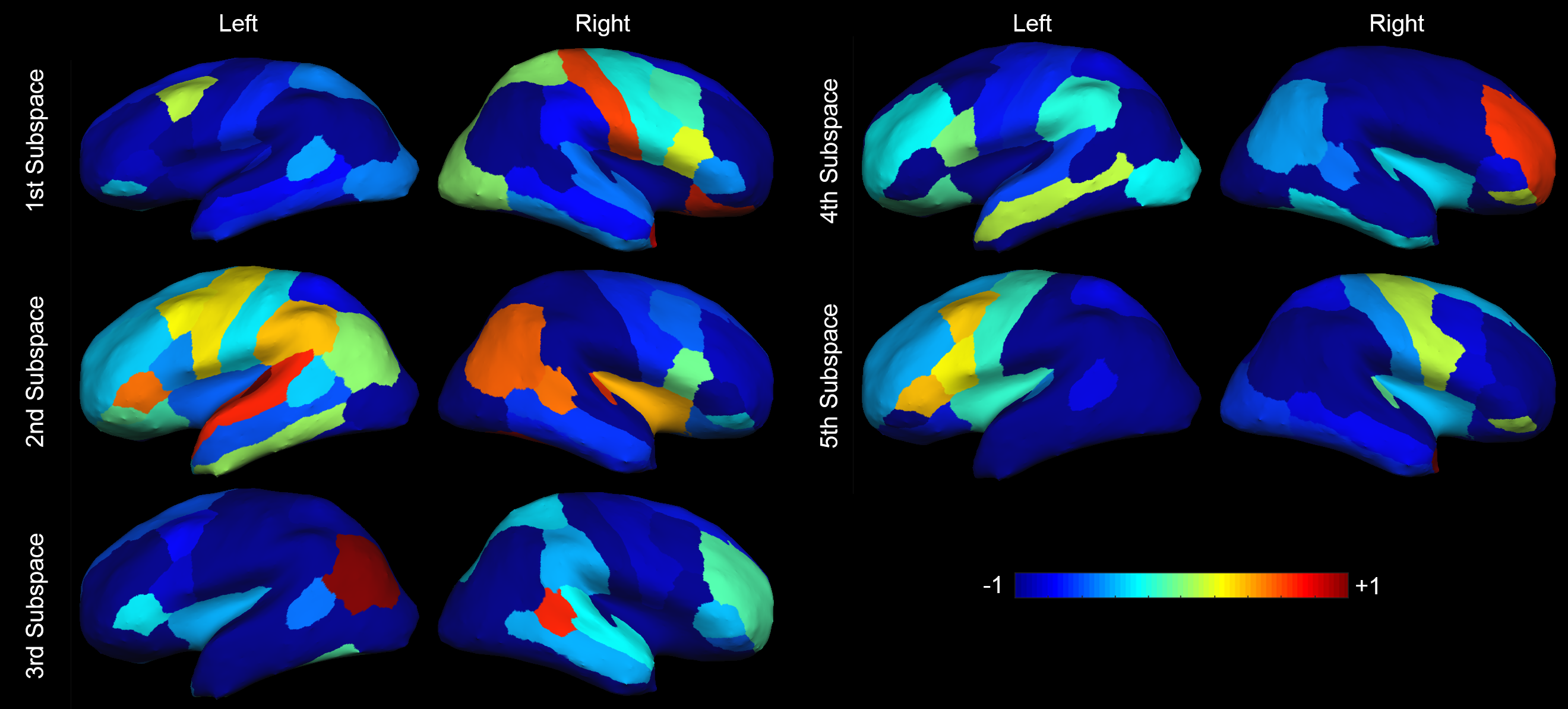
Figure 4. Brain mapping of 5 lowest-level subspaces identified in the proposed Subspace Network.

We find that each subspace captures very different information. In the first subspace, the volumes of right banks of the superior temporal sulcus, which is found to involve in prodromal AD (Killiany et al., 2000), rostral middle frontal gyrus, with highest A$\beta$ loads in AD pathology (Nicoll et al., 2003), and the volume of inferior parietal lobule, which was found to have an increased S-glutathionylated proteins in a proteomics study (Newman et al., 2007), have significant magnitude. We also find evidence of strong association between AD pathology and brain regions of large magnitude in other subspaces. The subspaces in remaining levels and detailed clinical analysis will be available in a journal extension of this paper.

5. Conclusions and future work

In this paper, we proposed a Subspace Network (SN), an efficient deep modeling approach for non-linear multi-task censored regression, where each layer of the subspace network performs a multi-task censored regression to improve upon the predictions from the last layer via sketching a low-dimensional subspace to perform knowledge transfer among learning tasks. We show that under mild assumptions, for each layer we can recover the parametric subspace using only one pass of training data. We demonstrate empirically that the subspace network can quickly capture correct parameter subspaces, and outperforms state-of-the-arts in predicting neurodegenerative clinical scores from brain imaging. Based on similar formulations, the proposed method can be easily extended to cases where the targets have nonzero bounds, or both lower and upper bounds.

Appendix

We hereby give more details for the proofs of both asymptotic and non-asymptotic convergence properties for Algorithm 1 to recover the latent subspace $U$. The proofs heavily rely on a series of previous results in (Mairal et al., 2010; Kasiviswanathan et al., 2012; Shalev-Shwartz et al., 2012; Mardani et al., 2013, 2015; Shen et al., 2016), and many key results are directly referred to hereinafter for conciseness. We include the proofs for the manuscript to be self-contained.

At iteration $i=1,2,...,N$, we sample $(x_{i},y_{i})$, and let $U^{i},V^{i}$ denote the intermediate $U$ and $V$, to be differentiated from $U_{t},V_{t}$ which are the $t$-th columns of $U,V$. For the proof feasibility, we assume that $\{(x_{i},y_{i})\}_{i=1}^{N}$ are sampled i.i.d., and the subspace sequence $\{U^{i}\}_{i=1}^{N}$ lies in a compact set.

Proof of Asymptotic Properties

For infinite data streams with $N\rightarrow\infty$, we recall the instantaneous cost of the $i$-th datum:

$$g_{i}(x_{i},y_{i},U,V)=-\log\Pr(x_{i},y_{i}|U,V)+\frac{\lambda}{2}\|U\|_{F}^{2}+\frac{\lambda}{2}\|V\|_{F}^{2},$$

and the online optimization form recasted as an empirical cost minimization:

$$\min\nolimits_{U}\frac{1}{N}\sum\nolimits_{i=1}^{N}g_{i}(x_{i},y_{i},U,V).$$

The Stochastic Gradient Descent (SGD) iterations can be seen as minimizing the approximate cost:

$$\min\nolimits_{U}\frac{1}{N}\sum\nolimits_{i=1}^{N}g^{\prime}_{i}(x_{i},y_{i},U,V).$$

where $g^{\prime}_{N}$ is a tight quadratic surrogate for $g_{N}$ based on the second-order Taylor approximation around $U^{N-1}$:

$$g^{\prime}_{N}(x_{N},y_{N},U,V) =g_{N}(x_{N},y_{N},U^{N-1},V)$$

$$+\langle\nabla_{U}g_{N}(x_{N},y_{N},U^{N-1},V),U-U^{N-1}\rangle$$

$$+\frac{\alpha_{N}}{2}\|U-U^{N-1}\|_{F}^{2},$$

with $\alpha_{N}\geq\|\nabla^{2}_{U}g_{N}(x_{N},y_{N},U^{N-1},V)\|$. $g^{\prime}_{N}$ is further recognized as a locally tight upper-bound surrogate for $g_{N}$, with locally tight gradients. Following the Appendix 1 of (Shen et al., 2016), we can show that $g_{N}$ is smooth, with its first-order and second-order gradients bounded w.r.t. each $U_{N}$.

With the above results, the convergence of subspace iterates can be proven in the same regime developed in (Mardani et al., 2015), whose main inspirations came from (Mairal et al., 2010) that established convergence of an online dictionary learning algorithm using the martingale sequence theory. In a nutshell, the proof procedure proceeds by first showing that $\sum_{i=1}^{N}g_{i}^{\prime}(x_{i},y_{i},U^{i},V^{i})$ converges to $\sum_{i=1}^{N}g_{i}(x_{i},y_{i},U^{i},V^{i})$ asymptotically, according to the quasi-martingale property in the almost sure sense, owing to the tightness of $g^{\prime}$. It then implies convergence of the associated gradient sequence, due to the regularity of $g$.

Meanwhile, we notice that $g_{i}(x_{i},y_{i},U,V)$ is bi-convex for the block variables $U_{t}$ and $V$ (see Lemma 2 of  (Shen et al., 2016)). Therefore due to the convexity of $g_{N}$ w.r.t. $V$ when $U=U^{N-1}$ is fixed, the parameter sketches $V$ can also be updated exactly per iteration.

All above combined, we can claim the asymptotic convergence for the iterations of Algorithm 1: as $N\rightarrow\infty$, the subspace sequence $\{U^{i}\}_{i=1}^{N}$ asymptotically converges to a stationary-point of the batch estimator, under a few mild conditions.

Proof of Non-Asymptotic Properties

For finite data streams, we rely on the unsupervised formulation of regret analysis  (Kasiviswanathan et al., 2012; Shalev-Shwartz et al., 2012) to assess the performance of online iterates. Specifically, at iteration $t$ ($t\leq N$), we use the previous $U^{t-1}$ to span the partial data at $i=1,2,...,t$. Prompted by the alternating nature of iterations, we adopt a variant of the unsupervised regret to assess the goodness of online subspace estimates in representing the partially available data. With $g_{t}(x_{t},y_{t},U^{t-1},V)$ being the loss incurred by the estimate $U^{t-1}$ for predicting the $t$-th datum, the cumulative online loss for a stream of size $T$ is given by:

(4) $$\bar{C}_{T}:=\frac{1}{T}\sum_{\tau=1}^{T}g_{\tau}(x_{\tau},y_{\tau},U^{\tau-1},V).$$

Further, we will assess the cost of the last estimate $U^{T}$ using:

(5) $$\hat{C}_{T}=\frac{1}{T}\sum_{\tau=1}^{T}g_{\tau}(x_{\tau},y_{\tau},U^{T},V).$$

We define $C_{T}$ as the batch estimator cost. For the sequence $\{U^{t}\}_{t=1}^{T}$, we define the online regret:

(6) $$\mathcal{R}_{T}:=\hat{C}_{T}-\bar{C}_{T}.$$

We investigate the convergence rate of the sequence $\{\mathcal{R}_{T}\}$ to zero as $T$ grows. Due to the nonconvexity of the online subspace iterates, it is challenging to directly analyze how fast the online cumulative loss $\bar{C}_{t}$ approaches the optimal batch cost $C_{t}$. As (Shen et al., 2016) advocates, we instead investigate whether $\hat{C}_{t}$ converges to $\bar{C}_{t}$. That is established by first referring to the Lemma 2 of (Mardani et al., 2013): the distance between successive subspace estimates will vanish as fast as $O(1/t)$: $\|U^{t}-U^{t-1}\|_{F}\leq\frac{B}{t}$, for some constant $B$ that is independent of $t$ and $N$. Following the proof of Proposition 2 in (Shen et al., 2016), we can similarly show that: if $\{U^{t}\}_{t=1}^{T}$ and $\{V_{t}x_{t}\}_{t=1}^{T}$ are uniformly bounded, i.e.,  $\|U^{t}\|_{F}\leq B_{1}$, and $\|V_{t}x_{t}\|_{2}\leq B_{2}$, $\forall t\leq T$, then with constants $B_{1},B_{2}>0$ and by choosing a constant step size $\mu_{t}=\mu$, we have a bounded regret as:

$$\mathcal{R}_{T}\leq \frac{B^{2}(\ln(T)+1)^{2}}{2\mu T}+\frac{5B^{2}}{6\mu T}.$$

This thus concluded the proof.

- (1)
- Adeli-Mosabbeb et al. (2015) Ehsan Adeli-Mosabbeb, Kim-Han Thung, Le An, Feng Shi, and Dinggang Shen. 2015. Robust feature-sample linear discriminant analysis for brain disorders diagnosis. In NIPS. 658–666.
- Argyriou et al. (2007) Andreas Argyriou, Theodoros Evgeniou, and Massimiliano Pontil. 2007. Multi-task feature learning. NIPS 19 (2007), 41.
- Association et al. (2013) Alzheimer’s Association et al. 2013. 2013 Alzheimer’s disease facts and figures. Alzheimer’s & dementia 9, 2 (2013), 208–245.
- Berberidis et al. (2016) Dimitris Berberidis, Vassilis Kekatos, and Georgios B Giannakis. 2016. Online censoring for large-scale regressions with application to streaming big data. TSP 64, 15 (2016), 3854–3867.
- Candes and Romberg (2007) Emmanuel Candes and Justin Romberg. 2007. Sparsity and incoherence in compressive sampling. Inverse problems 23, 3 (2007), 969.
- Caruana (1998) Rich Caruana. 1998. Multitask learning. In Learning to learn. Springer, 95–133.
- Cummings (1997) Jeffrey L Cummings. 1997. The Neuropsychiatric Inventory Assessing psychopathology in dementia patients. Neurology 48, 5 Suppl 6 (1997), 10S–16S.
- Desikan et al. (2006) Rahul S Desikan, Florent Ségonne, Bruce Fischl, et al. 2006. An automated labeling system for subdividing the human cerebral cortex on MRI scans into gyral based regions of interest. Neuroimage 31, 3 (2006), 968–980.
- Evgeniou and Pontil (2004) Theodoros Evgeniou and Massimiliano Pontil. 2004. Regularized multi–task learning. In SIGKDD. ACM, 109–117.
- He et al. (2016) Kaiming He, Xiangyu Zhang, Shaoqing Ren, and Jian Sun. 2016. Deep residual learning for image recognition. In CVPR. 770–778.
- Hughes et al. (1982) Charles P Hughes, Leonard Berg, Warren L Danziger, et al. 1982. A new clinical scale for the staging of dementia. The British journal of psychiatry 140, 6 (1982), 566–572.
- Jack et al. (2008) Clifford R Jack, Matt A Bernstein, Nick C Fox, Paul Thompson, et al. 2008. The Alzheimer’s disease neuroimaging initiative (ADNI): MRI methods. J. of mag. res. imag. 27, 4 (2008), 685–691.
- Jalali et al. (2010) Ali Jalali, Sujay Sanghavi, Chao Ruan, and Pradeep K Ravikumar. 2010. A dirty model for multi-task learning. In NIPS. 964–972.
- Kasiviswanathan et al. (2012) Shiva P Kasiviswanathan, Huahua Wang, Arindam Banerjee, and Prem Melville. 2012. Online l1-dictionary learning with application to novel document detection. In NIPS. 2258–2266.
- Killiany et al. (2000) Ronald J Killiany, Teresa Gomez-Isla, Mark Moss, Ron Kikinis, Tamas Sandor, Ferenc Jolesz, Rudolph Tanzi, Kenneth Jones, Bradley T Hyman, and Marilyn S Albert. 2000. Use of structural magnetic resonance imaging to predict who will get Alzheimer’s disease. Annals of neurology 47, 4 (2000), 430–439.
- Mairal et al. (2010) Julien Mairal, Francis Bach, Jean Ponce, and Guillermo Sapiro. 2010. Online learning for matrix factorization and sparse coding. JMLR 11, Jan (2010), 19–60.
- Mardani et al. (2013) Morteza Mardani, Gonzalo Mateos, and Georgios B Giannakis. 2013. Dynamic anomalography: Tracking network anomalies via sparsity and low rank. J. of Sel. To. in Sig. Proc. 7, 1 (2013), 50–66.
- Mardani et al. (2015) Morteza Mardani, Gonzalo Mateos, and Georgios B Giannakis. 2015. Subspace learning and imputation for streaming big data matrices and tensors. TSP 63, 10 (2015), 2663–2677.
- Martins et al. (2005) CAR Martins, A Oulhaj, CA De Jager, and JH Williams. 2005. APOE alleles predict the rate of cognitive decline in Alzheimer disease A nonlinear model. Neurology 65, 12 (2005), 1888–1893.
- Newman et al. (2007) Shelley F Newman, Rukhsana Sultana, Marzia Perluigi, Rafella Coccia, Jian Cai, William M Pierce, Jon B Klein, Delano M Turner, and D Allan Butterfield. 2007. An increase in S-glutathionylated proteins in the Alzheimer’s disease inferior parietal lobule, a proteomics approach. Journal of neuroscience research 85, 7 (2007), 1506–1514.
- Nicoll et al. (2003) James AR Nicoll, David Wilkinson, Clive Holmes, Phil Steart, Hannah Markham, and Roy O Weller. 2003. Neuropathology of human Alzheimer disease after immunization with amyloid- peptide: a case report. Nature medicine 9, 4 (2003), 448.
- Poulin et al. (2011) Stéphane P Poulin, Rebecca Dautoff, John C Morris, et al. 2011. Amygdala atrophy is prominent in early Alzheimer’s disease and relates to symptom severity. Psy. Res.: Neur. 194, 1 (2011), 7–13.
- Rosen et al. (1984) Wilma G Rosen, Richard C Mohs, and Kenneth L Davis. 1984. A new rating scale for Alzheimer’s disease. The American journal of psychiatry (1984).
- Sainath et al. (2013) Tara N Sainath, Brian Kingsbury, Vikas Sindhwani, et al. 2013. Low-rank matrix factorization for deep neural network training with high-dimensional output targets. In ICASSP. IEEE, 6655–6659.
- Scale—Fourth (2009) Wechsler D Wechsler Memory Scale—Fourth. 2009. Edition (WMS-IV). New York: Psychological Corporation (2009).
- Seltzer and Droppo (2013) Michael L Seltzer and Jasha Droppo. 2013. Multi-task learning in deep neural networks for improved phoneme recognition. In ICASSP. IEEE, 6965–6969.
- Shalev-Shwartz et al. (2012) Shai Shalev-Shwartz et al. 2012. Online learning and online convex optimization. Foundations and Trends® in Machine Learning 4, 2 (2012), 107–194.
- Shen et al. (2016) Yanning Shen, Morteza Mardani, and Georgios B Giannakis. 2016. Online Categorical Subspace Learning for Sketching Big Data with Misses. arXiv preprint arXiv:1609.08235 (2016).
- Srebro et al. (2005) Nathan Srebro, Jason Rennie, and Tommi S Jaakkola. 2005. Maximum-margin matrix factorization. In NIPS. 1329–1336.
- Sweet et al. (2012) Robert A Sweet, Howard Seltman, James E Emanuel, et al. 2012. Effect of Alzheimer’s disease risk genes on trajectories of cognitive function in the Cardiovascular Health Study. Ame. J. of Psyc. 169, 9 (2012), 954–962.
- Tombaugh and McIntyre (1992) Tom N Tombaugh and Nancy J McIntyre. 1992. The mini-mental state examination: a comprehensive review. Journal of the American Geriatrics Society 40, 9 (1992), 922–935.
- Wang et al. (2015) Zhangyang Wang, Jianchao Yang, Hailin Jin, et al. 2015. Deepfont: Identify your font from an image. In MM. ACM, 451–459.
- Wu et al. (2015) Zhizheng Wu, Cassia Valentini-Botinhao, Oliver Watts, and Simon King. 2015. Deep neural networks employing multi-task learning and stacked bottleneck features for speech synthesis. In ICASSP. IEEE, 4460–4464.
- Xue et al. (2013) Jian Xue, Jinyu Li, and Yifan Gong. 2013. Restructuring of deep neural network acoustic models with singular value decomposition.. In Interspeech. 2365–2369.
- Yang et al. (2010) Haiqin Yang, Irwin King, and Michael R Lyu. 2010. Online learning for multi-task feature selection. In CIKM. ACM, 1693–1696.
- Zhang et al. (2012) Daoqiang Zhang, Dinggang Shen, Alzheimer’s Disease Neuroimaging Initiative, et al. 2012. Multi-modal multi-task learning for joint prediction of multiple regression and classification variables in Alzheimer’s disease. NeuroImage 59, 2 (2012), 895–907.
- Zhang et al. (2013) Tianzhu Zhang, Bernard Ghanem, Si Liu, and Narendra Ahuja. 2013. Robust visual tracking via structured multi-task sparse learning. IJCV 101, 2 (2013), 367–383.
- Zhang et al. (2014) Zhanpeng Zhang, Ping Luo, Chen Change Loy, and Xiaoou Tang. 2014. Facial landmark detection by deep multi-task learning. In ECCV. Springer, 94–108.
- Zhou et al. (2011a) Jiayu Zhou, Jianhui Chen, and Jieping Ye. 2011a. Malsar: Multi-task learning via structural regularization. Arizona State University 21 (2011).
- Zhou et al. (2011b) Jiayu Zhou, Lei Yuan, Jun Liu, and Jieping Ye. 2011b. A multi-task learning formulation for predicting disease progression. In SIGKDD. ACM, 814–822.
- Zhou and Feng (2017) Zhi-Hua Zhou and Ji Feng. 2017. Deep forest: Towards an alternative to deep neural networks. arXiv preprint arXiv:1702.08835 (2017).