Anti-adiabatic evolution in quantum-classical hybrid system

Abstract

The adiabatic theorem is an important concept in quantum mechanics, it tells that a quantum system subjected to gradually changing external conditions remains to the same instantaneous eigenstate of its Hamiltonian as it initially in. In this paper, we study the another extreme circumstance where the external conditions vary rapidly such that the quantum system can not follow the change and remains in its initial state (or wavefunction). We call this type of evolution anit-adiabatic evolution. We examine the matter-wave pressure in this situation and derive the condition for such an evolution. The study is conducted by considering a quantum particle in an infinitely deep potential, the potential width $Q$ is assumed to be change rapidly. We show that the total energy of the quantum subsystem decreases as $Q$ increases, and this rapidly change exerts a force on the wall which plays the role of boundary of the potential. For $Q<Q_{0}$ ($Q_{0}$ is the initial width of the potential), the force is repulsive, and for $Q>Q_{0}$, the force is positive. The condition for the anti-adiabatic evolution is given via a spin-$\frac{1}{2}$ in a rotating magnetic field.

I introduction

A quantum system would remain in the instantaneous eigenstate of its Hamiltonian if the Hamiltonian changes slowly enough with respect to the energy gaps among the instantaneous eigenstate P. Ehrenfest16 ; M. Born28 ; J. Schwinger37 ; T. Kato50 . This is the so-called adiabatic theorem, which is an important and intuitive concept in quantum mechanics, and it was found insightful and potential to applications. For example, Landau-Zener transition, Berry phase L. D. Landau32 ; C. Zener32 ; M. Gell-mann51 ; M. V. Berry84 , quantum control and quantum adiabatic computationT.Corbitt07 ; M.Bhattacharya08 . Although progresses have been made, there are many issues remain open concerning the adiabatic evolution, for instance, the adiabatic condition K. P. Marzlin04 ; D. M. Tong05 and its extension to open systems yijpb07 .

Recent years have witnessed a series of developments at the intersection of optical cavities and mechanical resonatorscraighead00 ; aspelmeyer14 . The opto-mechanical coupling between a moving mirror and the radiation pressure of light has first appeared in the context of interferometric gravitational wave experiments. Owing to the discrete nature of photons, the quantum fluctuations of the radiation pressure forces give rise to the so-called standard quantum limitcaves81 . The experimental manifestations of opto-mechanical coupling by radiation pressure have been observable for some time. For instance, radiation pressure forces were observed indorsel83 , while even earlier work in the microwave domain had been carried out by Braginskybraginsky77 . Moreover the modification of mechanical oscillator stiffness caused by radiation pressure, the optical spring, have also recently been observedsheard04 .

It is the similarity between light and matter-wave that motivates the concept so-called matter-wave pressureJ.Shen10 . By examining the dynamics of the adiabatic quantum-classical system, the authors calculated the force exerted on the classical subsystem by the quantum subsystemJ.Shen10 . In the analysis, an assumption that the classical system moves slowly is used, this leads to the adiabatic evolution for the quantum subsystem.

On the contrary, quantum quenching refers to a sudden change of some parameter of the Hamiltonian. A variety of processes can result in quenching, such as a sudden moving of the mirror in optomechanics, a spin rotating driven by a magnetic field. Recently, the concept of phase transitions has been extended to non-equilibrium dynamics of time-independent systems induced by a quantum quencharkadiusz17 . It has been shown that the quantum quench in a discrete time crystal leads to dynamical quantum phase transitions, and the return probability of a periodically driven system to a Floquet eigenstate before the quench reveals singularities in time. Based on random quenches, random unitaries in atomic Hubbard and spin models can be generatedelben17 , this proposal works for a broad class of atomic and spin lattice modelsvermersch18 .

It is believe that in the case of rapidly varying conditions (to which the quantum system subjected), the quantum system may has no time to change its statecitro05 ; pellegrini11 ; eidelstein13 . If this is the case, what is the condition for such an evolution? Is it that the quantum system has no time to change its state? or it can not follow the rapidly changing conditions? How the matter-wave pressure behaves in this circumstance? In this paper, we will focus on these questions.

The paper is organized as follows. In Sec.II, we study the dynamics of a quantum particle in an infinitely deep potential with varying potential width. The matter-wave pressure force is calculated and discussed by assuming that the system remains in its initial state. In Sec.III, we derive the condition of anti-adiabatic evolution trough a simple example. Finally, we conclude our results in Sec.IV.

II a quantum particle in an infinite one-dimensional potential with varying width

Consider a quantum system in a one-dimensional infinitely deep well whose boundary at $Q$ is a moving wall(see Fig.1).

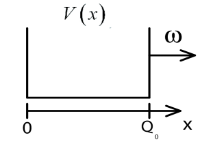
Figure 1: A infinitely deep potential well with a moving wall as its right boundary, the wall may move fast with respect to other parameters in the system, in particular the time scale of transitions among the particle-potential energy levels.

The Hamiltonian $\hat{H}$ of this system can be written as,

$$\hat{H}=-\frac{\hbar^{2}}{2m}\frac{d^{2}}{dx^{2}}+V(x),$$ (1)

where the potential $V(x)$ takes,

$$V(x)=\left\{\begin{array}[]{cc}0&0\leq x\leq Q\\ +\infty&x<0~{}\text{or}~{}x>Q\end{array}\right..$$ (4)

Suppose that the moving wall at $Q$ only changes the boundary condition of the quantum system, we have the eigenvalues and the corresponding eigenstates of the quantum system with fixed $Q$,

$$\Psi_{n}(Q)=\langle q|\psi_{n}(q,Q)\rangle=\sqrt{\frac{2}{Q}}\sin\frac{n\pi q}{Q},$$

$$E_{n}(Q)=\frac{\hbar^{2}\pi^{2}n^{2}}{2mQ^{2}},~{}~{}~{}~{}~{}n=1,2,3\cdots,$$ (5)

where $q$ denotes the coordinate of the quantum particle.

In the following, we assume that the wall moves so fast such that the quantum system does not evolve. The condition for this assumption to hold will be discussed in the next section. Suppose that the quantum particle is initially prepared in the ground state with the boundary at $Q_{0}$, i.e.,

$$\Psi_{1}(Q_{0})=\sqrt{\frac{2}{Q_{0}}}\sin\frac{\pi q}{Q_{0}},$$

$$E_{1}(Q_{0})=\frac{\hbar^{2}\pi^{2}}{2mQ_{0}^{2}}.$$ (6)

At next instance of time, the wall moves to $Q$. Since we assume the wall to moves so fast, the particle does not evolve and keeps in $\Psi_{1}(Q_{0})$ that can be expended as a function of $\Psi_{n}(Q)$,

$$\Psi_{1}(Q_{0})=\sum_{n}b_{n}\Psi_{n}(Q),~{}~{}~{}~{}~{}n=1,2,3,\cdots,$$ (7)

where $b_{n}$ is the expansion coefficients, and we define $\rho_{n}=|b_{n}|^{2}$, standing for the probability of the particle in the $n$th energy-level with the wall at $Q$. Simple calculation shows that,

$$b_{n}=\left\{\begin{array}[]{ll}\frac{(-1)^{n}2n\sqrt{\gamma}\sin(\gamma\pi)}{\pi(\gamma^{2}-n^{2})},&~{}~{}\gamma<1;\\ \frac{2\gamma^{\frac{3}{2}}}{\pi(\gamma^{2}-n^{2})}\sin\frac{n\pi}{\gamma},&~{}~{}\gamma>1\text{ and }n\neq\gamma;\\ \frac{1}{\sqrt{\gamma}},&~{}~{}n=\gamma.\end{array}\right.$$ (11)

where $\gamma=\frac{Q}{Q_{0}}$ was defined. $\rho_{n}$ follows from Eq.(11),

$$\rho_{n}=\left\{\begin{array}[]{ll}\frac{4n^{2}\gamma\sin^{2}(\gamma\pi)}{\pi^{2}(\gamma^{2}-n^{2})^{2}},&~{}~{}\gamma<1;\\ \frac{4\gamma^{3}}{\pi^{2}(\gamma^{2}-n^{2})^{2}}\sin^{2}(\frac{n\pi}{\gamma}),&~{}~{}\gamma>1\text{ and }n\neq\gamma;\\ \frac{1}{\gamma},&~{}~{}n=\gamma.\end{array}\right.$$ (15)

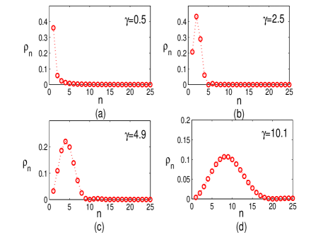
Figure 2: (Color on line) The population $\rho_{n}$ as a function of n, where the energy level is calculated with the boundary at $Q$. Where $\gamma$ are taken as 0.5, 1.5, 4.9 and 10.1 respectively.

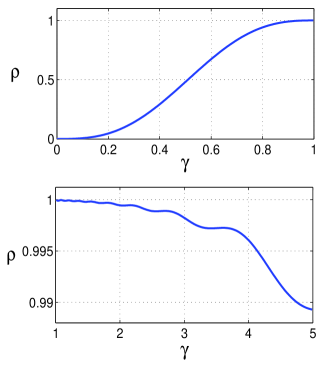
Figure 3: (Color on line) The total probability of the first ten energy-levels.

From Eq.(15), we find that the probability $\rho_{n}$ is only a function of $\gamma$ and $n$, indicating that $Q$ and $Q_{0}$ jointly changes $\rho_{n}$. Furthermore, expression for $0<\gamma<1$ and $\gamma>1$ is different. In Fig.2 we plot the probability distribution over the energy level $\Psi_{n}(Q)$, while $\gamma$ is chosen to 0.5, 1.5, 4.9 and 10.1, respectively. From this figure, we find that there are population transfer from the ground state to the higher energy levels that is different from the results in Ref.J.Shen10 . We also find that the probability distribution sharply depends on $\gamma$. For example, when $\gamma=4.9$, the particle mainly occupied the 5th level, while the occupation of the other levels, especially that far from the 5th levels, are almost zero. From Eq.(5), we observe that the $n$th eigenfunction with boundary at $Q$ is similar to the initial state when $n\approx\gamma$. This may be the reason why the probability of the energy-level with index (i.e., $n$) close to $\gamma$ is favoringly occupied.

To calculate the energy change due to boundary moving, we have to calculate the population distribution over all eigenstates of the Hamiltonian with the new boundary. This is a time-consuming task. Fortunately, our calculation show that only first 10 levels are populated when the boundary change is from $0$ to $5Q_{0}$(see Fig.3). Then we can only take the first ten energy-levels into account, which is a good approximation to calculating the energy for the parameter under our discussion.

Since $\Psi_{1}$ can be expended as Eq.(7), we can easily get the total energy after the boundary moving to the new position,

$$E^{{}^{\prime}} = \sum_{n=1}^{10}\rho_{n}^{{}^{\prime}}E_{n}^{{}^{\prime}}$$ (16)

$$= \sum_{n=1}^{10}\frac{\rho_{n}}{\sum_{n=1}^{10}\rho_{n}}E_{n}^{{}^{\prime}}$$

$$= \sum_{n=1}^{10}\frac{\rho_{n}}{\sum_{n=1}^{10}\rho_{n}}\frac{\hbar^{2}\pi^{2}n^{2}}{2m(\gamma Q_{0})^{2}}$$

$$= \sum_{n=1}^{10}\frac{\rho_{n}}{\sum_{n=1}^{10}\rho_{n}}\frac{n^{2}}{\gamma^{2}}\cdot E_{1},$$

where $\rho^{{}^{\prime}}$ is the re-normalized probability distribution over the first ten energy-levels.

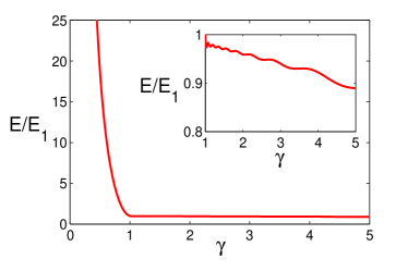
Figure 4: (Color on line) The energy (in units of $E_{1}$) of the atom as a function of the ratio $\frac{Q}{Q_{0}}$ with the initial condition $Q_{0}=1.0$ (in units of nm) and $E_{1}=5.49*10^{-23}j$($m=10^{-27}kg,h=6.626*10^{-34}j\cdot s$).

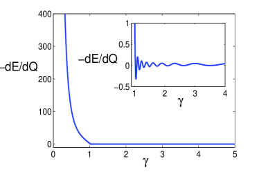
Figure 5: (Color on line) The force(in units of $\frac{E_{1}}{Q_{0}}$) between the quantum subsystem and the classical subsystem with $Q$ is in units of nm and the energy $E$ is in units of $E_{1}$, where $E_{1}=5.49*10^{-23}j$($m=10^{-27}kg,h=6.626*10^{-34}j\cdot s$).

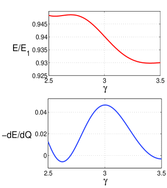
Figure 6: (Color on line) A local graphics amplification of Fig.4 and Fig.5 from $\gamma=2.5$ to $\gamma=3.5$.

From Eq.(15) and Eq.(16), we find that $E^{{}^{\prime}}$ depends only on $\gamma$ and $n$. In other words, $E^{{}^{\prime}}$ does not depends on $Q$ and $Q_{0}$ separately. So it is interesting to see how the ratio $\gamma$ affects the total energy when the boundary changes rapidly.

Fig.4 shows the dependence of the energy on $\gamma$. We find that the total energy increases rapidly as $\gamma$ decreases in the regime $0<\gamma<1$. This observation can be easily understood by examining Eq.(5). It is obviously that $E_{n}$ is inversely proportional to the square of the width of the well $Q$, which means that the energy of each energy-level increases as $Q$ decreases and $Q<Q_{0}$. Moreover, because we choose the ground state as the initial state, no matter in what state the particle will be after the boundary change, the total energy will certainly increases.

For $\gamma>1$, the situation is different. We find that the total energy decreases at large as $\gamma$ increases. The total energy change is almost zero when the change of $Q$ is not very large. Meanwhile we find that the energy does change monotonically with $\gamma$. In other words, the energy may increase as $\lambda$ increases. This is interesting. In Ref.J.Shen10 , the total energy decreases as $\gamma$ increases. This is because the evolution of the system is adiabatic and the particle is always at the ground state of the Hamiltonian, no matter how the boundary changes. In the other words, the width of the well $Q$ is the only parameter to determine the energy of the quantum subsystem. However, this is not the case for anti-adiabatic evolution in our model. Indeed, there are population transfer among the eigenstates when the boundary changes from $Q_{0}$ to $Q$, see Eq.(7). Namely the particle will not always stay in the ground state when the boundary changes. This will affect the total energy of the system. From Eq.(16), we can see that the total energy is related to $b_{n}$, which varies as the boundary changes. This analysis suggests that the energy depends on two parameters, one the eigenvalue $E_{n}$ and the other is the population distribution $\rho_{n}$. From Eq.(5), we can see that when $Q$ increases, the eigenvalue $E_{n}(Q)$ decreases. On the other hand, from Eqs.(11) and (15), we see that the change of $\gamma$ will result in the change of the population $\rho_{n}$. Specifically, we find that the probability distribution mainly in a few energy levels near $\gamma$ for $\gamma>1$. These together can interpret why the total energy increase as $Q$ increases. see Fig.4.

Now we discuss this issue from the aspect of matter wave force exerted on the boundary wall. It can be given by $F=-\frac{dE}{dQ}$ J.Shen10 . We show this force in Fig. 5. From Fig.5, we find that the force tends to very large and repulsive as $Q$ decreases in the regime $Q<Q_{0}$. This is similar to the result in Ref.J.Shen10 . In addition, for the case of $Q>Q_{0}$, the force has a slight fluctuation around zero with the increasing of $Q$. This means that the force between the particle and the moving wall may be repulsive or attractive. Fig.6 is a enlarged version of Fig.4 and Fig.5 for $\gamma$ ranging from $\gamma=2.5$ to $\gamma=3.5$. From the two figures, we observe that when the total energy increases, the force is attractive. On the contrary, there is a repulsive force when the total energy decreases. Since the change of the total energy due to the boundary moving is so weak for $Q>Q_{0}$, the force in this case is negligibly small.

III a spin-$\frac{1}{2}$ in a rotating magnetic field

In the last section, we study the matter-wave pressure with an assumption that the boundary moves so fast that the quantum system does not evolve. One may wonder if this situation exist, and what is the condition for such an evolution. Does the system have no time to evolve? Or the change is too fast that the system can not follow? To simplify the discussion, we here adapt a simple model that a spin-$\frac{1}{2}$ in a rotating magnetic field to formulate the problem.

The system Hamiltonian takes, $\hat{H}=-\vec{\mu}\cdot\vec{B(t)}$. We will choose $\vec{B(t)}=B_{0}\widehat{n(t)}$ with the unit vector $\widehat{n(t)}=(\sin\alpha\cos\omega t,\sin\alpha\sin\omega t,\cos\alpha)$ as the magnetic field, where $B_{0}$ is strength of the field. The eigenvalue and the corresponding eigenstate of the system takes,

$$\mathbf{\psi_{1}}(t) = (\cos(\alpha/2),e^{i\omega t}\sin(\alpha/2))^{T},$$

$$E_{1} = +\frac{\hbar\omega_{0}}{2}$$ (17)

and

$$\mathbf{\psi_{2}}(t) = (e^{-i\omega t}\sin(\alpha/2),-\cos(\alpha/2))^{T},$$

$$E_{2} = -\frac{\hbar\omega_{0}}{2}$$ (18)

where $E_{1}$ and $E_{2}$ are the eigenvalues of $\mathbf{\psi_{1}}$ and $\mathbf{\psi_{2}}$, respectively. And $\omega$ is the frequency of the magnetic field, $\alpha$ denotes the angle between the spin and the magnetic field. $\omega_{0}\equiv\frac{eB_{0}}{m}$, and $e$ is the charge of the particle, $m$ is the mass of the particle. Starting with $\mathbf{\psi_{1}}(t=0)$, the particle will evolve to

$$\mathbf{\psi}(t)=\left(\begin{array}[]{c}(\cos(\frac{\lambda t}{2})-i(\frac{\omega_{0}-\omega}{\lambda})\sin(\frac{\lambda t}{2}))\cos(\frac{\alpha}{2})e^{-\frac{i\omega t}{2}}\\ (\cos(\frac{\lambda t}{2})-i(\frac{\omega_{0}+\omega}{\lambda})\sin(\frac{\lambda t}{2}))\sin(\frac{\alpha}{2})e^{\frac{i\omega t}{2}}\\ \end{array}\right)$$ (19)

where $\lambda$ is defined by,

$$\lambda=\sqrt{\omega^{2}+\omega_{0}^{2}-2\omega\omega_{0}\cos(\alpha)}.$$ (20)

We now examine in which circumstance the system remains un-evolved on $\mathbf{\psi_{1}(0)}$. This can be done by calculating the probability of the particle on $\mathbf{\psi_{1}(0)}$,

$$\rho_{1}(t) = |\langle\mathbf{\psi}(t)|\mathbf{\psi_{1}(0)}\rangle|^{2}$$ (21)

$$= [\cos(\frac{\lambda t}{2})\sin(\frac{\omega t}{2})\cos\alpha$$

$$+(\frac{\omega_{0}-\omega\cos\alpha}{\lambda})\sin(\frac{\lambda t}{2})\cos(\frac{\omega t}{2})]^{2}$$

$$+[\cos(\frac{\lambda t}{2})\cos(\frac{\omega t}{2})$$

$$+(\frac{\omega-\omega_{0}\cos\alpha}{\lambda})\sin(\frac{\lambda t}{2})\sin(\frac{\omega t}{2})]^{2}.$$

We are interested in the probability of the particle in its initial state, when the magnetic filed completes a circle. Eq.(21) would give the results if we assume that the evolution time $t$ and the magnetic frequency $\omega$ satisfy $\omega t=2\pi$. With $\omega t=2\pi$, Eq.(21) can be rewritten as

$$\rho_{1}(\omega) = \cos^{2}(\frac{\lambda\pi}{\omega})+(\frac{\omega_{0}-\omega\cos\alpha}{\lambda})^{2}\sin^{2}(\frac{\lambda\pi}{\omega}).$$ (22)

On the contrary, the particle will evolve to $\mathbf{\psi^{{}^{\prime}}(t)}$ given blow when starting with $\mathbf{\psi_{2}}(t=0)$,

$$\mathbf{\psi}^{{}^{\prime}}(t)=\left(\begin{array}[]{c}(\cos(\frac{\lambda t}{2})+i(\frac{\omega_{0}+\omega}{\lambda})\sin(\frac{\lambda t}{2}))\sin(\frac{\alpha}{2})e^{-\frac{i\omega t}{2}}\\ -(\cos(\frac{\lambda t}{2})+i(\frac{\omega_{0}-\omega}{\lambda})\sin(\frac{\lambda t}{2}))\cos(\frac{\alpha}{2})e^{\frac{i\omega t}{2}}\\ \end{array}\right)$$ (23)

$$\rho_{2}^{{}^{\prime}}(t) = |\langle\mathbf{\psi}^{{}^{\prime}}(t)|\mathbf{\psi_{2}(0)}\rangle|^{2}$$ (24)

$$= [\cos(\frac{\lambda t}{2})\sin(\frac{\omega t}{2})\cos\alpha$$

$$+(\frac{\omega_{0}-\omega\cos\alpha}{\lambda})\sin(\frac{\lambda t}{2})\cos(\frac{\omega t}{2})]^{2}$$

$$+[\cos(\frac{\lambda t}{2})\cos(\frac{\omega t}{2})$$

$$+(\frac{\omega-\omega_{0}\cos\alpha}{\lambda})\sin(\frac{\lambda t}{2})\sin(\frac{\omega t}{2})]^{2}.$$

$$\rho_{2}^{{}^{\prime}}(\omega) = \cos^{2}(\frac{\lambda\pi}{\omega})+(\frac{\omega_{0}-\omega\cos\alpha}{\lambda})^{2}\sin^{2}(\frac{\lambda\pi}{\omega}).$$ (25)

From Eqs(24) and (25), we observe that the expressions of $\rho_{2}^{{}^{\prime}}(t)$ and $\rho_{2}^{{}^{\prime}}(\omega)$ both are the same as $\rho_{1}(t)$ and $\rho_{1}(\omega)$. Hence, we only discuss the evolution of $\psi(t)$ in the following discussions.

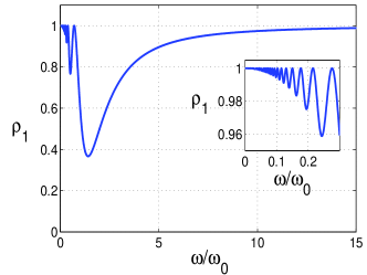
Figure 7: (Color on line) The relationship between $\rho_{1}$ and $\omega$ with $\alpha=\frac{\pi}{4}$, $\omega_{0}\equiv\frac{\mathbf{e}B_{0}}{m}$ being a c-frequency and $B_{0}=1~{}T$, where $e~{}(-1.6\times 10^{-19}~{}c)$ is the charge of the electron and $m~{}(9.3\times 10^{-31}~{}kg)$ is the mass of the electron.

In Fig.7, we plot $\rho_{1}$ as a function of $\omega$ for $\alpha=\frac{\pi}{4}$. From this figure, we can find that when $\frac{\omega}{\omega_{0}}$ is very small, the evolution of $\rho_{1}$ is irregular, for this reason we can not find a suitable frequency $\omega$ to make sure that the electron will stay in the initial state. Fortunately, $\rho_{1}$ increases with the increasing of $\omega$ when $\frac{\omega}{\omega_{0}}>1.442$ and we find that when $\omega$ is 15 times larger than $\omega_{0}$, the probability $\rho_{1}$ is almost one and we claim that the electron will stay at the state $\mathbf{\psi_{1}}(0)$ at any time. This suggests that the quantum system will stay in its initial state if the external conditions change much faster than the typical frequency of the system.

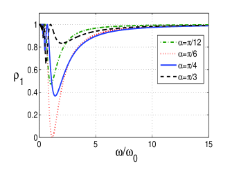
Figure 8: (Color on line) The relationship between $\rho_{1}$ and $\omega$ with $\alpha=\frac{\pi}{12},\frac{\pi}{6},\frac{\pi}{4}$ and $\frac{\pi}{3}$, respectively. And $\omega_{0}\equiv\frac{\mathbf{e}B_{0}}{m}$ being a c-frequency and $B_{0}=1~{}T$, where $e~{}(-1.6\times 10^{-19}~{}c)$ is the charge of the electron and $m~{}(9.3\times 10^{-31}~{}kg)$ is the mass of the electron.

In Fig.8, we plot $\rho_{1}$ as a function of $\omega$ for different $\alpha$. From this figure, we find that the minimum value of $\rho_{1}$ changes for different $\alpha$. However, there always exists a $\omega$ which can keep the system at the state $\mathbf{\psi_{1}}(0)$ at any time, no matter what $\alpha$ is. And $\omega$ for different $\alpha$ is nearly the same.

IV Conclusion and discussions

The adiabatic theorem tells that a quantum mechanical system subjected to gradually changing external conditions can adapt its functional form. In this paper, we explore another extreme varying conditions–rapidly varying conditions. The evolution of the system in this condition we call anti-adiabatic evolution. We have examined the condition for such evolutions and calculate the matter-wave pressure for the quantum system. Specifically, we have considered a quantum particle in a one-dimensional infinitely deep potential, one boundary of the potential is assumed to move rapidly, such that the particle inside does not evolve with time, however, as the potential width varies, the energy of the particle changes. This change would lead to a force on the quantum system. We calculated the force and find that as the width increases the force is attractive, while it is repulsive as the width decreases. By considering a spin-$\frac{1}{2}$ in a rotating magnetic field, we explore the condition for the anti-adiabatic evolution. Discussions and remarks on this condition are given.

References

- (1) P. Ehrenfest, Ann. Phys (Berlin) 51,327 (1916).
- (2) M. Born and V. Fock, Z.Phys 51,165 (1928).
- (3) J. Schwinger, Phys. Rev 51,648 (1937).
- (4) T. Kato, J. Phys .Soc. Jpn 5,435 (1950).
- (5) L. D. Landau, Zeitschrify 2,46 (1932).
- (6) C. Zener, Proc. R. Soc. London A 137,696 (1932).
- (7) M. Gell-mann and F. Low, Phys. Rev 84,350 (1951).
- (8) M. V. Berry, Proc. R. Soc. A 392,45 (1984).
- (9) T. Corbitt, Y. Chen, E. Innerhofer, H. Müller-Ebhardt, D. Ottaway, H. Rehbein, D. Sigg, S. Whitcomb, C. Wipf, and N. Mavalvala, Phys. Rev. Lett. 98, 150802 (2007).
- (10) M. Bhattacharya, H. Uys and P. Meystre, Phys. Rev. A 77, 033819 (2008).
- (11) K. P. Marzlin and B. C. Sanders, Phys. Rev. Lett. 93,160408 (2004).
- (12) D. M. Tong, K. Singh, L. C. Kwek, and C. H. Oh, Phys. Rev. Lett. 95, 110407 (2005).
- (13) X. X. Yi, D. M. Tong, L. C. Kwek, and C. H. Oh, J. Phys. B 40, 281 (2007).
- (14) H. G. Craighead, Science 290, 1532 (2000).
- (15) Markus Aspelmeyer, Tobias J. Kippenberg, and Florian Marquardt, Cavity optomechanics, Rev. Mod. Phys. 86, 1391 (2014), and references therein.
- (16) C. M. Caves, Physical Review D 23, 1693(1981); K. Jacobs, I. Tittonen, H. M. Wiseman, and S. Schiller, Physical Review A 60, 538(1999); I. Tittonen, G. Breitenbach, T. Kalkbrenner, T. Muller, R. Conradt, S. Schiller, E. Steinsland, N. Blanc, and N. F. de Rooij, Physical Review A 59, 1038(1999).
- (17) A. Dorsel, J. D. McCullen, P. Meystre, E. Vignes, and H. Walther, Physical Review Letters 51, 1550(1983).
- (18) V. B. Braginsky, Measurement of Weak Forces in Physics Experiments (University of Chicago Press, Chicago, 1977).
- (19) B. S. Sheard, M. B. Gray, C. M. Mow-Lowry, D. E. McClelland, and S. E. Whitcomb, Observation and characterization of an optical spring, Phys. Rev. A 69, 051801(R) (2004).
- (20) J. Shen, X. L. Huang, X. X. Yi, Chunfeng Wu, and C. H. Oh, Phys. Rev. A 82, 062107 (2010).
- (21) Arkadiusz Kosior and Krzysztof Sacha, Dynamical quantum phase transitions in discrete time crystals, arXiv:1712.05588v1.
- (22) A. Elben, B. Vermersch, M. Dalmonte, J. I. Cirac, and P. Zoller, arXiv:1709.05060.
- (23) B. Vermersch, A. Elben, M. Dalmonte, J. I. Cirac, and P. Zoller, Unitary n-designs via random quenches in atomic Hubbard and Spin models: Application to the measurement of R nyi entropies, arXiv:1801.00999v1.
- (24) R. Citro, E. Orignac, T. Giamarchi, Adiabatic-antiadiabatic crossover in a spin-Peierls chain, Phys. Rev. B 72, 024434 (2005).
- (25) Franco Pellegrini, Carlotta Negri, Fabio Pistolesi, Nicola Manini, Giuseppe E. Santoro, Erio Tosatti, Crossover from adiabatic to antiadiabatic quantum pumping with dissipation, Phys. Rev. Lett. 107, 060401 (2011).
- (26) Eitan Eidelstein, Dotan Goberman, Avraham Schiller, Crossover from adiabatic to antiadiabatic phonon-assisted tunneling in single-molecule transistors, Phys. Rev. B 87, 075319 (2013).