Equidistribution of zeros of polynomials

Abstract.

A classical result of Erdős and Turán states that if a monic polynomial has small size on the unit circle and its constant coefficient is not too small, then its zeros cluster near the unit circle and become equidistributed in angle. Using Fourier analysis we give a short and self-contained proof of this result.

1. Introduction.

Any set of $N$ complex numbers may be viewed as the zero set of a polynomial of degree $N$. If, however, we start with a polynomial that “arises naturally”—for example, think of polynomials with coefficients $\pm 1$—then the zeros will tend to be “evenly distributed near the unit circle.” In [6], Erdős and Turán proved the beautiful result that if the size of a monic polynomial on the unit circle is small, and its constant term is not too small, then its zeros cluster around the unit circle and become equally distributed in sectors. We shall make precise both the hypothesis and conclusion of this statement later, but we hope Figure 1 gives an impression of the phenomenon. The Erdős-Turán result was subsequently refined by Ganelius [7] and Mignotte [11], and in this note we give a short and self-contained proof, obtaining as a bonus a modest improvement of the previous results.

Let

$$P(z)=\prod_{j=1}^{N}(z-\alpha_{j})=z^{N}+a_{N-1}z^{N-1}+\cdots+a_{0}$$

be a polynomial of degree $N$, and write the roots $\alpha_{j}$ as $\alpha_{j}=\rho_{j}e^{i\theta_{j}}$. It may be helpful to think first of situations where the roots are not equidistributed near the unit circle. For example, one could have the polynomial $(z-1)^{N}=\sum_{j=0}^{N}(-1)^{j}\binom{N}{j}z^{j}$, where all the roots are concentrated at one point $z=1$ and clearly not spread out evenly. This polynomial has large coefficients, and on the unit circle it attains a maximum size of $2^{N}$. A different type of example is the polynomial $z^{N}-1/2^{N}$. Here the polynomial takes only small values on the unit circle, but all the roots are on the circle with radius $1/2$. A more extreme version of this example is the polynomial $z^{N}$.

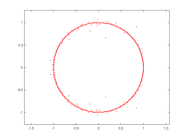
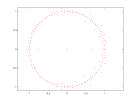
Figure 1. Left: Zeros of a polynomial of degree $500$ formed with the decimal digits of $\pi$: $3z^{500}+z^{499}+4z^{498}+\cdots$. Right: Zeros of the Fekete polynomial $\sum_{j=0}^{162}(\frac{j}{163})z^{j}$ where the coefficients are given by the Legendre symbol $(\frac{j}{163})=\pm 1$ for $1\leq j\leq 162$.

These examples indicate that it would be necessary to assume that the size of $P$ on the unit circle must be small, and that the constant term $a_{0}$ should not be too small in order to establish equidistribution of zeros. Henceforth we will assume that $a_{0}\neq 0$ so that the roots $\alpha_{j}$ are all nonzero. One convenient measure of the size of coefficients is the quantity

$$H(P)=\max_{|z|=1}\frac{|P(z)|}{\sqrt{|a_{0}|}}.$$

The triangle inequality gives, with the convention $a_{N}=1$,

$$H(P)\leq\frac{1}{\sqrt{|a_{0}|}}\sum_{j=0}^{N}|a_{j}|.$$

On the other hand, Parseval’s formula gives

$$H(P)^{2}=\max_{|z|=1}\frac{|P(z)|^{2}}{|a_{0}|}\geq\frac{1}{|a_{0}|}\frac{1}{2\pi}\int_{0}^{2\pi}|P(e^{i\theta})|^{2}d\theta=\frac{1}{|a_{0}|}\sum_{j=0}^{N}|a_{j}|^{2}.$$

Combining our upper bound for $H(P)$ with the Cauchy–Schwarz inequality we find that

(1) $$\frac{1}{|a_{0}|}\sum_{j=0}^{N}|a_{j}|^{2}\leq H(P)^{2}\leq\frac{N}{|a_{0}|}\sum_{j=0}^{N}|a_{j}|^{2}.$$

Assuming that $H(P)$ is small is therefore equivalent to assuming that the coefficients of $P$ are small and that the constant coefficient $a_{0}$ is not too small. Here by “small” we mean that $H(P)$ is not exponentially large in $N$; for example, one could think of a condition like $H(P)\leq e^{\epsilon N}$ for suitably small $\epsilon$. In fact, we shall formulate the Erdős–Turán theorem in terms of the slightly more refined quantity

$$h(P)=\frac{1}{2\pi}\int_{0}^{2\pi}\log^{+}\frac{|P(e^{i\theta})|}{\sqrt{|a_{0}|}}d\theta,\qquad\text{where}\qquad\log^{+}x=\max(0,\log x).$$

Since $H(P)\geq(|a_{0}|^{2}+|a_{N}|^{2})/|a_{0}|=(|a_{0}|^{2}+1)/|a_{0}|\geq 1$ in view of the lower bound in (1), the quantity $h(P)$ satisfies

$$h(P)\leq\log\max_{|z|=1}\frac{|P(z)|}{\sqrt{|a_{0}|}}=\log H(P),$$

so that the assumption that $h(P)$ is small is weaker than the assumption that $H(P)$ is small.

We now turn to the question of how to quantify the idea that zeros are equidistributed around the unit circle. We do this in two stages, first discussing the magnitude of zeros, and then discussing the spacings of their arguments. To treat the magnitude of the zeros (recall $\alpha_{j}=\rho_{j}e^{i\theta_{j}}$), we define

$${\mathcal{M}}(P)=\prod_{j=1}^{N}\max\Big{(}\rho_{j},\frac{1}{\rho_{j}}\Big{)}.$$

As an easy consequence of Jensen’s formula from complex analysis, we shall establish the following upper bound for ${\mathcal{M}}(P)$ in terms of $h(P)$.

Theorem 1.

With notations as above,

$${\mathcal{M}}(P)\leq\exp(2h(P)).$$

To gain a sense of this result, suppose we knew the upper bound ${\mathcal{M}}(P)\leq\exp(\epsilon^{2}N)$. Then it would follow that at most $\epsilon N$ zeros can lie outside the band $e^{-\epsilon}\leq|z|\leq e^{\epsilon}$. Or, in other words, most of the zeros will lie inside a narrow band around the unit circle.

The more difficult part of the Erdős–Turán theorem concerns the equidistribution of the angles $\theta_{j}$. Given an arc $I$ on the unit circle, let $N(I;P)$ denote the number of zeros $\alpha_{j}$ with $e^{i\theta_{j}}$ lying on this arc. If the angles $\theta_{j}$ are equidistributed, then we may expect $N(I;P)$ to be roughly $\frac{N}{2\pi}$ times the length of the arc $I$ (which we will denote by $|I|$). A convenient way to measure equidistribution is the discrepancy, which is defined as

$${\mathcal{D}}(P)=\max_{I}\Big{|}N(I;P)-\frac{|I|}{2\pi}N\Big{|}.$$

In other words, the discrepancy measures the worst case deviation of the actual count of the number of angles lying on a given arc from the number that one would expect if the angles were equidistributed. A bound ${\mathcal{D}}(P)\leq\epsilon N$, for suitably small $\epsilon$, would indicate that the angles $\theta_{j}$ are evenly distributed.

Theorem 2.

With notations as above,

(2) $${\mathcal{D}}(P)\leq\frac{8}{\pi}\sqrt{Nh(P)}.$$

Theorems 1 and 2 together establish that if $h(P)$ is small compared to $N$, then the zeros of $P$ cluster around the unit circle and become equidistributed in angle. For example, if the coefficients of $P$ are always $\pm 1$, then since $H(P)\leq N+1$, it follows from Theorem 1 that ${\mathcal{M}}(P)\leq(N+1)^{2}$, and from Theorem 2 that ${\mathcal{D}}(P)\leq\frac{8}{\pi}\sqrt{N\log(N+1)}$.

Erdős and Turán [6] first established a version of (2), with the constant $8/\pi$ replaced by $16$ and with $\log H(P)$ instead of $h(P)$. Ganelius [7] showed an estimate like (2), again with $\log H(P)$ instead of $h(P)$, but with a better constant than Erdős and Turán, namely with $\sqrt{2\pi/k}=2.5619\ldots$ (with $k=1/1^{2}-1/3^{2}+1/5^{2}-\cdots=0.9159\ldots$ denoting the Catalan constant) instead of $16$. Mignotte [11] refined Ganelius’s result, replacing $\log H(P)$ by the sharper $h(P)$. Note that our theorem sharpens the Ganelius–Mignotte result slightly, since $8/\pi=2.5464\ldots$ is a little smaller than $\sqrt{2\pi/k}$. There is some scope to improve the constant $8/\pi$ (especially in the situation where $h(P)$ is small compared to $N$), but Amoroso and Mignotte [2] have produced examples showing that the constant in (2) must be at least $\sqrt{2}$.

There is a vast literature surrounding zeros of polynomials, and we give a few references to related work. For the distribution of zeros of polynomials with $0$, $1$ coefficients see [13]; for work on “Fekete polynomials” where the coefficients equal the Legendre symbol $\pmod{p}$, see [4]; for work on random polynomials with coefficients drawn independently from various distributions (where Theorems 1 and 2 will apply with high probability), see [9]; for two recent variants on the Erdős–Turán theorem, see [15] and [5]. While the Erdős–Turán result applies to all polynomials with complex coefficients, in number theory greater interest is attached to irreducible polynomials with integer coefficients. If $P(x)=a_{N}x^{N}+\cdots+a_{0}\in{\mathbb{Z}}[x]$ is a polynomial with roots $\alpha_{j}$, then a central object here is the Mahler measure which is $M(P)=|a_{N}|\prod_{j=1}^{N}\max(1,|\alpha_{j}|)$. A beautiful result of Bilu [3] states that if $P$ is an irreducible polynomial in ${\mathbb{Z}}[x]$ and $M(P)\leq(1+\epsilon)^{N}$ is not large, then the zeros of $P$ cluster near the unit circle and are equidistributed; for a gentle exposition, see [8]. Any discussion of zeros of polynomials would be incomplete without a mention of Lehmer’s outstanding open problem that the smallest value of $M(P)$ that is larger than $1$ is $M(L)=1.1762\ldots$, attained for Lehmer’s polynomial $L(x)=x^{10}+x^{9}-x^{7}-x^{6}-x^{5}-x^{4}-x^{3}+x+1$; for a recent comprehensive survey, see [14]. Finally, our proof uses ideas from Fourier analysis; two lovely books in this area are [10] and [12].

2. Jensen’s formula and the proof of Theorem 1.

We begin with the easier result, Theorem 1, which follows from Jensen’s formula. If $f$ is holomorphic in a domain containing the unit disk with $f(0)\neq 0$, then Jensen’s formula (see 5.3.1 of Ahlfors [1]) states that

$$\frac{1}{2\pi}\int_{0}^{2\pi}\log|f(e^{i\theta})|d\theta=\log|f(0)|+\sum_{j}\log\frac{1}{|z_{j}|},$$

where the sum is over the zeros $z_{j}$ of $f$ lying inside the unit disk.

Applying Jensen’s formula, and since $P(0)=a_{0}$, we find

$$\frac{1}{2\pi}\int_{0}^{2\pi}\log\frac{|P(e^{i\theta})|}{\sqrt{|a_{0}|}}d\theta=\frac{1}{2}\log|a_{0}|+\sum_{\rho_{j}<1}\log\frac{1}{\rho_{j}}.$$

But $|a_{0}|=\prod_{j=1}^{N}\rho_{j}$, and so the above also equals

$$-\frac{1}{2}\log|a_{0}|+\sum_{\rho_{j}>1}\log\rho_{j}.$$

Adding these two expressions,

$$2\Big{(}\frac{1}{2\pi}\int_{0}^{2\pi}\log\frac{|P(e^{i\theta})|}{\sqrt{|a_{0}|}}d\theta\Big{)}=\sum_{j}\log\max\Big{(}\frac{1}{\rho_{j}},\rho_{j}\Big{)}$$

and, since the left side above is clearly at most $2h(P)$, Theorem 1 follows.

3. An observation of Schur.

The rest of this article is devoted to proving Theorem 2. We begin with an observation attributed to Schur (see [2]) that will allow us to restrict attention to polynomials with all zeros on the unit circle.

Lemma 3.

Let $P(z)=\prod_{j=1}^{N}(z-\alpha_{j})$ with $\alpha_{j}=\rho_{j}e^{i\theta_{j}}$ be as above, and define the polynomial $Q$ by $Q(z)=\prod_{j=1}^{N}(z-e^{i\theta_{j}})$. Then for any $z$ with $|z|=1$, we have

$$\frac{|P(z)|}{\sqrt{|a_{0}|}}\geq|Q(z)|,$$

so that $h(P)\geq h(Q)$.

Proof.

Observe that for any $z$ with $|z|=1$,

$$\Big{|}\frac{z}{\sqrt{\rho_{j}}}-\sqrt{\rho_{j}}e^{i\theta_{j}}\Big{|}^{2}=\frac{1}{\rho_{j}}+\rho_{j}-2\text{Re }ze^{-i\theta_{j}}\geq 2-2\text{Re }ze^{-i\theta_{j}}=|z-e^{i\theta_{j}}|^{2},$$

and so

$$\frac{|P(z)|}{\sqrt{|a_{0}|}}=\prod_{j=1}^{N}\Big{|}\frac{z}{\sqrt{\rho_{j}}}-\sqrt{\rho_{j}}e^{i\theta_{j}}\Big{|}\geq\prod_{j=1}^{N}|z-e^{i\theta_{j}}|=|Q(z)|,$$

proving the lemma. ∎

Since the discrepancies ${\mathcal{D}}(P)$ and ${\mathcal{D}}(Q)$ are the same, and since $h(P)\geq h(Q)$, it is enough to establish Theorem 2 for the polynomial $Q$ and then the corresponding bound for the polynomial $P$ would follow. In other words, we may assume from now on that all zeros of $P$ lie on the unit circle, so that $\rho_{j}=1$ for all $j$.

4. Smoothed sums over the zeros.

Let $P(z)=\prod_{j=1}^{N}(z-e^{i\theta_{j}})$ be a polynomial of degree $N$ with all zeros on the unit circle. The following lemma establishes a crucial link between the power sums of the zeros (by which we mean $\sum_{j=1}^{N}e^{ik\theta_{j}}$ for integers $k$) and the size of $P$ on the unit circle.

Lemma 4.

Let $P(z)=\prod_{j=1}^{N}(z-e^{i\theta_{j}})$ be as above. For any integer $k\neq 0$ we have

(3) $$\sum_{j=1}^{N}e^{ik\theta_{j}}=-\frac{|k|}{\pi}\int_{0}^{2\pi}e^{ik\theta}\log|P(e^{i\theta})|d\theta.$$

Consequently, for any integer $k\neq 0$,

(4) $$\Big{|}\sum_{j=1}^{N}e^{ik\theta_{j}}\Big{|}\leq 4|k|h(P).$$

The link between power sums of the roots and the size of $P$ should not come as a surprise—Newton’s identities connecting power sums of the roots with the coefficients of a polynomial are a different version of such a link. For our purposes the identity (3) will, however, be much more useful than Newton’s identities. For a general polynomial $P(z)=\prod_{j=1}^{N}(z-\rho_{j}e^{i\theta_{j}})$, the relation (3) may be replaced by

$$\sum_{j=1}^{N}\min\Big{(}\rho_{j},\frac{1}{\rho_{j}}\Big{)}^{|k|}e^{ik\theta_{j}}=-\frac{|k|}{\pi}\int_{0}^{2\pi}e^{ik\theta}\log\frac{|P(e^{i\theta})|}{\sqrt{|a_{0}|}}d\theta.$$

Proof of Lemma 4.

For any real number $\phi$ and nonzero integer $k$, we shall show that

(5) $$e^{ik\phi}=-\frac{|k|}{\pi}\int_{0}^{2\pi}e^{ik\theta}\log|e^{i\theta}-e^{i\phi}|d\theta,$$

and then (3) follows upon summing this over all $\phi=\theta_{j}$. Substituting $\theta=x+\phi$, and dividing both sides by $e^{ik\phi}$, we see that (5) follows from the identity

$$1 =-\frac{|k|}{\pi}\int_{0}^{2\pi}e^{ikx}\log|e^{ix}-1|dx=-\frac{|k|}{\pi}\int_{0}^{2\pi}e^{ikx}\log(2\sin(x/2))dx$$

(6) $$=-\frac{|k|}{\pi}\int_{0}^{2\pi}\cos(kx)\log(2\sin(x/2))dx,$$

where the last step follows upon pairing $x$ and $2\pi-x$. Since $\cos$ is an even function, it is enough to establish (4) in the case when $k$ is positive. Integration by parts shows that the right-hand side of (4) equals

$$-\frac{1}{\pi}\int_{0}^{2\pi}\log(2\sin(x/2))d\sin(kx)=\frac{1}{2\pi}\int_{0}^{2\pi}\frac{\sin kx}{\sin(x/2)}\cos(x/2)dx.$$

Since

$$\frac{\sin kx}{\sin(x/2)}=\frac{e^{ikx}-e^{-ikx}}{e^{ix/2}-e^{-ix/2}}=2\sum_{j=1}^{k}\cos\Big{(}\frac{2j-1}{2}x\Big{)},$$

it follows that

$$\frac{1}{2\pi}\int_{0}^{2\pi}\frac{\sin kx}{\sin(x/2)}\cos(x/2)dx=\sum_{j=1}^{k}\frac{1}{\pi}\int_{0}^{2\pi}\cos\Big{(}\frac{2j-1}{2}x\Big{)}\cos(x/2)dx=1,$$

which proves (4), and therefore also (5) and (3).

The triangle inequality gives

$$\Big{|}\sum_{j=1}^{N}e^{ik\theta_{j}}\Big{|}\leq\frac{|k|}{\pi}\int_{0}^{2\pi}\Big{|}\log|P(e^{i\theta})|\Big{|}d\theta.$$

Now

$$\frac{1}{2\pi}\int_{0}^{2\pi}\Big{|}\log|P(e^{i\theta})|\Big{|}d\theta =\frac{1}{2\pi}\int_{0}^{2\pi}\Big{(}2\log^{+}|P(e^{i\theta})|-\log|P(e^{i\theta})|\Big{)}d\theta$$

(7) $$=2h(P),$$

upon recalling the definition of $h(P)$, and upon noting that Jensen’s formula gives $\int_{0}^{2\pi}\log|P(e^{i\theta})|d\theta=0$. This establishes (4). ∎

The reader familiar with Weyl’s equidistribution theorem (see Chapter 3 of [10] for an introduction) will recognize at once the significance of Lemma 4. The estimate (4) shows that if $h(P)$ is known to be small compared to $N$, then so are the power sums $\sum_{j=1}^{N}e^{ik\theta_{j}}$, at least for small values of $k$. Weyl’s criterion then gives the equidistribution $\mod{2\pi}$ of the angles $\theta_{j}$. Our goal now is to flesh out this argument; the general procedure is standard, but a few refinements are introduced to obtain Theorem 2 in its clean form.

Let $I$ be an arc on the unit circle, and let ${\mathcal{I}}(\theta)$ denote the indicator function for the arc $I$, which is $2\pi$-periodic. Thus, ${\mathcal{I}}(\theta)=1$ if $e^{i\theta}\in I$ and $0$ otherwise. We are interested in the number of zeros lying on the arc $I$:

$$N(I;P)=\sum_{j=1}^{N}{\mathcal{I}}(\theta_{j}).$$

Since ${\mathcal{I}}$ is periodic, it is tempting to invoke its Fourier expansion. This is a little delicate, since the function ${\mathcal{I}}$ is discontinuous and its Fourier series is not absolutely convergent. Instead we will work with “smoothed sums over zeros” $\sum_{j=1}^{N}g(\theta_{j})$ where $g$ is a $2\pi$-periodic function with better behaved Fourier series, and then choose $g$ to be a suitable approximation to the indicator function ${\mathcal{I}}$.

Proposition 5.

Let $P(z)=\prod_{j=1}^{N}(z-e^{i\theta_{j}})$ be as above. Let $g(\theta)$ be a $2\pi$-periodic continuous function such that

$$\sum_{k=-\infty}^{\infty}|k{\widehat{g}}(k)|<\infty,$$

where

$${\widehat{g}}(k)=\frac{1}{2\pi}\int_{0}^{2\pi}g(\theta)e^{-ik\theta}d\theta$$

denotes the Fourier coefficients of $g$. Put

$$G(\theta)=\sum_{k=-\infty}^{\infty}|k|{\widehat{g}}(k)e^{ik\theta}\qquad\text{and}\qquad G=\max_{\theta}|G(\theta)|.$$

Then

$$\Big{|}\sum_{j=1}^{N}g(\theta_{j})-\frac{N}{2\pi}\int_{0}^{2\pi}g(\theta)d\theta\Big{|}\leq 4Gh(P).$$

If the $2\pi$-periodic function $g$ is $\ell$-times continuously differentiable, then integration by parts $\ell$ times gives (for $k\neq 0$)

$$|{\widehat{g}}(k)|=\Big{|}\frac{1}{(ik)^{\ell}}\frac{1}{2\pi}\int_{0}^{2\pi}g^{(\ell)}(\theta)e^{-ik\theta}d\theta\Big{|}\leq\frac{1}{|k|^{\ell}}\max_{\theta\in[0,2\pi)}|g^{(\ell)}(\theta)|.$$

Thus, for example, any thrice continuously differentiable function will meet the hypothesis of Proposition 5 and there is a rich supply of such functions.

Proof of Proposition 5.

Using the Fourier expansion of $g$, we obtain

$$\sum_{j=1}^{N}g(\theta_{j})-\frac{N}{2\pi}\int_{0}^{2\pi}g(\theta)d\theta=\sum_{k\neq 0}{\widehat{g}}(k)\sum_{j=1}^{N}e^{ik\theta_{j}},$$

and so by Lemma 4 this equals

$$-\sum_{k\neq 0}{\widehat{g}}(k)\frac{|k|}{\pi}\int_{0}^{2\pi}e^{ik\theta}\log|P(e^{i\theta})|d\theta=-\frac{1}{\pi}\int_{0}^{2\pi}\log|P(e^{i\theta})|\sum_{k\neq 0}|k|{\widehat{g}}(k)e^{ik\theta}d\theta.$$

From the definition of $G$, in magnitude the above is bounded by

$$\frac{G}{\pi}\int_{0}^{2\pi}\Big{|}\log|P(e^{i\theta})|\Big{|}d\theta =\frac{G}{\pi}\int_{0}^{2\pi}\Big{(}2\log^{+}|P(e^{i\theta})|-\log|P(e^{i\theta})|\Big{)}d\theta$$

$$=4Gh(P),$$

upon recalling (4). ∎

To pave the way for the proof of Theorem 2 in the next section, we work out the bound of Proposition 5 for a particular class of functions $g$. The idea is that one can construct functions $g$ meeting the hypothesis of Proposition 5 by convolving the indicator function ${\mathcal{I}}$ with suitable nice functions ${\mathcal{K}}$. In the next section, we shall make a specific choice for ${\mathcal{K}}$ so that the resulting function $g$ approximates the indicator function ${\mathcal{I}}$ well.

Lemma 6.

Let $I$ be an arc on the unit circle, and let ${\mathcal{I}}(\theta)$ denote its indicator function as above. Let ${\mathcal{K}}$ be a $2\pi$-periodic continuous function that is always nonnegative, and whose Fourier coefficients ${\widehat{\mathcal{K}}}(n)$ are all nonnegative, with $\sum_{n\in{\mathbb{Z}}}{\widehat{\mathcal{K}}}(n)<\infty$. Let $g$ be the convolution of ${\mathcal{I}}$ and ${\mathcal{K}}$. Thus,

$$g(\theta)=\frac{1}{2\pi}\int_{0}^{2\pi}{\mathcal{I}}(\alpha){\mathcal{K}}(\theta-\alpha)d\alpha.$$

Then, $g$ satisfies the hypothesis of Proposition 5, and in the notation used there,

$$G=\max_{\theta}\Big{|}\sum_{k=-\infty}^{\infty}|k|{\widehat{g}}(k)e^{ik\theta}\Big{|}\leq\frac{2}{\pi^{2}}{\mathcal{K}}(0).$$

Proof.

Suppose that ${\mathcal{I}}$ is the arc from $e^{i\alpha}$ to $e^{i\beta}$, so that for $k\neq 0$ we have

$${\widehat{\mathcal{I}}}(k)=\frac{1}{2\pi}\int_{\alpha}^{\beta}e^{-iky}dy=\frac{e^{-ik\alpha}-e^{-ik\beta}}{2\pi ik}.$$

The Fourier coefficients of the convolution of two functions are the products of the Fourier coefficients of those functions; thus ${\widehat{g}}(k)={\widehat{\mathcal{I}}}(k){\widehat{\mathcal{K}}}(k)$. Therefore $|k{\widehat{g}}(k)|=|k{\widehat{\mathcal{I}}}(k)|{\widehat{\mathcal{K}}}(k)\leq{\widehat{\mathcal{K}}}(k)/\pi$ so that

$$\sum_{k=-\infty}^{\infty}|k{\widehat{g}}(k)|\leq\frac{1}{\pi}\sum_{k=-\infty}^{\infty}{\widehat{\mathcal{K}}}(k)=\frac{1}{\pi}{\mathcal{K}}(0)<\infty.$$

This shows that the hypothesis $\sum_{k}|k{\widehat{g}}(k)|<\infty$ in Proposition 5 is satisfied, and moreover establishes the bound $G\leq{\mathcal{K}}(0)/\pi$.

To obtain the more precise bound for $G$ claimed in our lemma, note that

$$G(\theta) =\sum_{k=-\infty}^{\infty}|k|{\widehat{g}}(k)e^{ik\theta}=\sum_{k=-\infty}^{\infty}|k|{\widehat{\mathcal{K}}}(k){\widehat{\mathcal{I}}}(k)e^{ik\theta}$$

$$=\frac{1}{2\pi i}\sum_{\begin{subarray}{c}k=-\infty\\ k\neq 0\end{subarray}}^{\infty}\text{sgn}(k){\widehat{\mathcal{K}}}(k)(e^{ik(\theta-\alpha)}-e^{ik(\theta-\beta)}).$$

Pairing the terms $k$ and $-k$ together, and using ${\widehat{\mathcal{K}}}(k)={\widehat{\mathcal{K}}}(-k)$ (since ${\mathcal{K}}$ and ${\widehat{\mathcal{K}}}$ are real valued), we find

$$|G(\theta)| =\frac{1}{2\pi}\Big{|}\sum_{\begin{subarray}{c}k=-\infty\\ k\neq 0\end{subarray}}^{\infty}\text{sgn}(k){\widehat{\mathcal{K}}}(k)\Big{(}\sin(k(\theta-\alpha)-\sin(k(\theta-\beta)\Big{)}\Big{|}$$

$$\leq 2\max_{\phi}\frac{1}{2\pi}\sum_{k=-\infty}^{\infty}{\widehat{\mathcal{K}}}(k)|\sin(k\phi)|.$$

Therefore

$$G=\max_{\theta}|G(\theta)|\leq 2\max_{\phi}\frac{1}{2\pi}\sum_{k=-\infty}^{\infty}{\widehat{\mathcal{K}}}(k)|\sin(k\phi)|.$$

A simple calculation gives the Fourier expansion

$$|\sin x|=\frac{2}{\pi}-\frac{4}{\pi}\sum_{\ell=1}^{\infty}\frac{\cos(2\ell x)}{4\ell^{2}-1},$$

and so we obtain

$$\frac{1}{2\pi}\sum_{k=-\infty}^{\infty}{\widehat{\mathcal{K}}}(k)|\sin(k\phi)| =\frac{1}{2\pi}\sum_{k=-\infty}^{\infty}{\widehat{\mathcal{K}}}(k)\Big{(}\frac{2}{\pi}-\frac{4}{\pi}\sum_{\ell=1}^{\infty}\frac{\cos(2k\ell\phi)}{4\ell^{2}-1}\Big{)}$$

$$=\frac{1}{\pi^{2}}{\mathcal{K}}(0)-\frac{2}{\pi^{2}}\sum_{\ell=1}^{\infty}\frac{{\mathcal{K}}(2\ell\phi)}{4\ell^{2}-1}\leq\frac{1}{\pi^{2}}{\mathcal{K}}(0),$$

proving the lemma. ∎

5. Proof of Theorem 2.

Let $I$ be an arc on the unit circle. To establish (2) it is enough to show that

(8) $$N(I;P)-\frac{|I|}{2\pi}N\leq\frac{8}{\pi}\sqrt{Nh(P)}.$$

Once the upper bound is in place, we may use that

$$N(I;P)-|I|N/(2\pi)=|I^{c}|N/(2\pi)-N(I^{c};P),$$

where $I^{c}$ denotes the arc complementary to $I$, to obtain a corresponding lower bound, and thus complete the proof of Theorem 2.

Let $g$ be a $2\pi$-periodic function that majorizes the indicator function of $I$; that is, $g(\theta)\geq 0$ always, and $g(\theta)\geq 1$ if $e^{i\theta}\in I$. Then

$$N(I;P)- \frac{|I|}{2\pi}N\leq\sum_{j=1}^{N}g(\theta_{j})-\frac{|I|}{2\pi}N$$

(9) $$=\Big{(}\sum_{j=1}^{N}g(\theta_{j})-\frac{N}{2\pi}\int_{0}^{2\pi}g(\theta)d\theta\Big{)}+N\Big{(}\frac{1}{2\pi}\int_{0}^{2\pi}g(\theta)d\theta-\frac{|I|}{2\pi}\Big{)}.$$

Now the strategy is to find a nice function $g$ for which we can use Proposition 5 and Lemma 6 to bound the first term above, while also keeping $g$ close to the indicator function of $I$ so that the second term is also small.

Given $\pi>\delta>0$, let $I_{\delta}$ denote the arc obtained by widening $I$ on either side by $\delta$. (If $|I|+2\delta>2\pi$ then take $I_{\delta}$ to be all of the unit circle.) Let us denote by ${\mathcal{I}}_{\delta}$ the indicator function of the widened arc $I_{\delta}$. Let ${\mathcal{K}}_{\delta}$ denote the $2\pi$-periodic function, given by

$${\mathcal{K}}_{\delta}(\theta)=\frac{2\pi}{\delta^{2}}\max(\delta-|\theta|,0)$$

for $\theta\in(-\pi,\pi]$. The function ${\mathcal{K}}_{\delta}$ is closely related to the Fejer kernel (see, for example, Chapter 2 of [10]), and its Fourier coefficients are easily computed: ${\widehat{\mathcal{K}}}_{\delta}(0)=1$, and for $k\neq 0$

$${\widehat{\mathcal{K}}_{\delta}}(k)=\Big{(}\frac{\sin(k\delta/2)}{k\delta/2}\Big{)}^{2}.$$

Take $g$ to be the convolution of ${\mathcal{I}}_{\delta}$ and ${\mathcal{K}}_{\delta}$; thus $g(\theta)=\frac{1}{2\pi}\int_{0}^{2\pi}{\mathcal{I}}_{\delta}(\alpha){\mathcal{K}}_{\delta}(\theta-\alpha)d\alpha$. From the definition of ${\mathcal{K}}_{\delta}$, and noting that $\frac{1}{2\pi}\int_{0}^{2\pi}{\mathcal{K}}_{\delta}(\alpha)d\alpha=1$, we see easily that the function $g(\theta)$ is always nonnegative, and it equals $1$ if $e^{i\theta}\in I$. We may think of $g$ as the indicator function ${\mathcal{I}}$ “smeared out” over a $\delta$ neighborhood of the arc $I$. If we make $\delta$ smaller, our approximation $g$ is closer to ${\mathcal{I}}$ and the second term on the right in (5) will become smaller, but, on the other hand, the function $g$ will become “less smooth” and the first term on the right in (5) will become larger. The idea is to choose $\delta$ optimally so as to balance these two effects.

Note that

$${\widehat{g}}(0)=\frac{1}{2\pi}\int_{0}^{2\pi}g(\theta)d\theta=\frac{|I_{\delta}|}{2\pi}=\frac{|I|+2\delta}{2\pi},$$

unless $I_{\delta}$ is all of the unit circle in which case ${\widehat{g}}(0)=1$. Since $g$ majorizes the indicator function of $I$, we may use (5), and from our evaluation of ${\widehat{g}}(0)$ it follows that the second term in the right side of (5) is at most $N\delta/\pi$.

To bound the first term in (5), we appeal to Proposition 5 and Lemma 6. They show that

$$\Big{|}\sum_{j=1}^{N}g(\theta_{j})-\frac{N}{2\pi}\int_{0}^{2\pi}g(\theta)d\theta\Big{|} \leq 4h(P)\max_{\theta}\Big{|}\sum_{k=-\infty}^{\infty}|k|{\widehat{g}}(k)e^{ik\theta}\Big{|}$$

$$\leq\frac{8}{\pi^{2}}{\mathcal{K}}_{\delta}(0)h(P)=\frac{16}{\pi\delta}h(P).$$

We conclude that

$$\sum_{j=1}^{N}g(\theta_{j})-\frac{|I|}{2\pi}N\leq\frac{16}{\pi\delta}h(P)+\frac{\delta}{\pi}N,$$

and choosing $\delta=4\sqrt{h(P)/N}$, the estimate (8) follows. The proof of Theorem 2 is now complete.

We conclude by looking back at the proofs, and pointing out the key steps. Theorem 1, showing that the roots accumulate near the unit circle, was a simple application of Jensen’s formula. The more difficult Theorem 2, which gives the equidistribution of the angles of the roots, began with an observation of Schur allowing us to restrict attention to the case when all roots lie on the unit circle. Then the key identity is contained in Lemma 2, which connects power sums of the roots with the size of the polynomial on the unit circle. Lemma 2 allows us to understand smooth sums over the angles of the roots, as in Proposition 1. The last step is the passage from smooth sums over angles to identifying angles lying on arcs, and this is carried out in Lemma 3 together with the work of this section.

Acknowledgment. I am grateful to Emanuel Carneiro, Persi Diaconis, Andrew Granville, Emmanuel Kowalski, Chen Lu, Pranav Nuti, and the referees for helpful comments, and especially to Pranav Nuti for producing Figure 1. I am partially supported by a grant from the National Science Foundation, and a Simons Investigator grant from the Simons Foundation. Part of the paper was written while the author was a Gauss Visiting Professor at Göttingen; I thank the University, and the Akademie der Wissenschaften zu Göttingen for their generous hospitality.

References

[1] Ahlfors, L.V. (1978). Complex analysis, third edition, McGraw-Hill Book Co., New York.
[2] Amoroso, F., Mignotte, M. (1996). On the distribution of the roots of polynomials. Ann. Inst. Fourier (Grenoble) 46(5): 1275–1291.
[3] Bilu, Y. (1997). Limit distribution of small points on algebraic tori. Duke Math. J. 89(3): 465–476.
[4] Conrey, B., Granville, A., Poonen, B., Soundararajan, K. (2000). Zeros of Fekete polynomials. Ann. Inst. Fourier (Grenoble) 50(3): 865–889.
[5] Erdélyi, T. (2008). An improvement of the Erdős–Turán theorem on the distribution of zeros of polynomials. C. R. Math. Acad. Sci. Paris 346(5-6): 267–270.
[6] Erdős, P., Turán, P. (1950). On the distribution of roots of polynomials. Ann. of Math. 51: 105–119.
[7] Ganelius, T. (1954). Sequences of analytic functions and their zeros. Ark. Mat., 3:1–50.
[8] Granville, A. (2007). The distribution of roots of a polynomial. In Equidistribution in number theory, an introduction,
volume 237 of NATO Sci. Ser. II Math. Phys. Chem., pages 93–102. Springer, Dordrecht.
[9] Hughes, C.P., Nikeghbali, A. (2008). The zeros of random polynomials cluster uniformly near the unit circle. Compos. Math. 144(3): 734–746.
[10] Körner, T.W. (1988). Fourier analysis. Cambridge University Press, Cambridge.
[11] Mignotte, M. (1992). Remarque sur une question relative à des fonctions conjuguées. C. R. Acad. Sci. Paris Sér. I. Math. 315(8):907–911.
[12] Montgomery, H.L. (2014). Early Fourier analysis, volume 22 of Pure and Aplied Undergraduate Texts. American Math. Soc., Providence, RI.
[13] Odlyzko, A.M., Poonen, B. (1993). Zeros of polynomials with , coefficients. Enseign. Math. 39(3-4): 317–348.
[14] Smyth, C. (2008). The Mahler measure of algebraic numbers: a survey. In Number theory and polynomials, volume 352 of London Math. Soc. Lecture Note Ser., pages 322–349. Cambridge University Press, Cambridge.
[15] Totik, V., Varjú, P. (2007). Polynomials with prescribed zeros and small norm. Acta Sci. Math. (Szeged) 73(3-4): 593–611.