Compiling Diderot: From Tensor Calculus to C

Abstract

Diderot is a parallel domain-specific language for analysis and visualization of multidimensional scientific images, such as those produced by CT and MRI scanners [12, 28]. In particular, it supports algorithms where tensor fields (i.e., functions from 3D points to tensor values) are used to represent the underlying physical objects that were scanned by the imaging device. Diderot supports higher-order programming where tensor fields are first-class values and where differential operators and lifted linear-algebra operators can be used to express mathematical reasoning directly in the language. While such lifted field operations are central to the definition and computation of many scientific visualization algorithms, to date they have required extensive manual derivations and laborious implementation.

The challenge for the Diderot compiler is to effectively translate the high-level mathematical concepts that are expressible in the surface language to a low-level and efficient implementation in C. This paper describes our approach to this challenge, which is based around the careful design of an intermediate representation (IR), called EIN, and a number of compiler transformations that lower the program from tensor calculus to C while avoiding combinatorial explosion in the size of the IR. We describe the challenges in compiling a language like Diderot, the design of EIN, and the transformation used by the compiler. We also present an evaluation of EIN with respect to both compiler efficiency and quality of generated code.

1 Introduction

Diderot is a domain-specific language for writing image-analysis algorithms that are defined using the concepts of differential tensor calculus and linear algebra [12, 28]. The design of Diderot couples a simple portable parallelism model with a very-high-level mathematical programming notation, which allows a user to directly transfer her mathematical reasoning from whiteboard to code. For example, a CT scan can be viewed as a 3D scalar tensor field $F$ (i.e., a continuous map from $\Re^{3}$ to scalar values), where the expression $F(x)$ represents the opacity to X-rays of the scanned object at point $x$. Using the concepts of tensor calculus, we can compute geometric properties of the scanned object. For our example, if the point $x$ lies on an isosurface in $F$, such as the boundary between hard and soft materials, the surface-normal vector at $x$ can be computed using the expression $-\nabla{}F(x)/|\nabla{}F(x)|$.

As in mathematics (and in functional programming), Diderot lifts operations on tensors (e.g., inner product) to work on tensor fields. Lifted operations allow programmers a more concise expression of their algorithmic ideas and allows them to avoid the tedious and error-prone by-hand lowering of higher-order operations to first-order code [10]. In these ways, Diderot provides a very-high-level mathematical programming model for computing with 2D and 3D image data.

The challenge of implementing Diderot is bridging the wide semantic gap from its very-high-level programming notation to the low-level code produced by the compiler. This paper describes an effective approach to this challenge that is based on an intermediate representation called EIN and a complementary set of optimizations and transformations. Many optimizing compilers rely on a normalized representation (e.g., SSA [15], ANF [21], or CPS [4]) where operations are applied to atomic values and intermediate results are given names, while other compilers have used expression trees to represent computation [24, 33]. In the design of EIN, we take a hybrid approach, where we embed an extensible family of operators that are defined by indexed expression trees inside an SSA-based IR. As we show, this hybrid approach allows a concise representation of the nested loops that arise in tensor computations, it supports the transformations necessary for implementing Diderot’s higher-order features, and it enables easier extension of the language, thus providing a solid foundation for future growth of the language.

The remainder of the paper is organized as follows. In the next section, we provide necessary background material, including a description of the computational core of Diderot, the mathematical foundations of this core, and an outline of the Diderot compiler’s architecture. We then describe the motivation for the work presented in the paper in Section 3. Sections 4 and 5 are the cover the main results of the paper: the design of our IR and its implementation in the compiler. In Section 6, we present an empirical evaluation of the compiler and the various choices of optimization. The main benefit of this work is that it supports a much more expressive programming model; in Section 7 we describe two algorithmic techniques that are enabled by the EIN IR. Related work is described in Section 8 followed by a conclusion.

2 Diderot

In this section, we given an overview of the Diderot language and explain the underlying techniques for representing continuous tensor fields that are reconstructed from multidimensional image data.

2.1 The Diderot Language

For this paper, we are primarily concerned with the computational core of Diderot; more complete descriptions of the language design can be found in previous papers [12, 28], and tutorial examples can be found on the Diderot example repository on GitHub (https://github.com/Diderot-Language/examples). The computational core is mostly organized around two families of types:

tensors

are concrete values that include scalars (0th-order), vectors (1st-order), matrices (2nd-order), and higher-order tensors. The Diderot type “tensor[$d_{1},\,\ldots,\,d_{n}$]” is the type of $n$th-order tensors in $\mathbb{R}{}^{d_{1}}\times\cdots\times\mathbb{R}{}^{d_{n}}$, where $n\geq 0$. We refer to $d_{1},\,\ldots,\,d_{n}$ as the shape of the tensor and will use $\sigma$ to denote shapes when the individual dimensions are not important. Also, we require that the dimensions $d_{i}$ satisfy $d_{i}>1$ to ensure that shapes are canonical.

tensor fields

are continuous functions from $\mathbb{R}{}^{d}$, where $1\leq d\leq 3$, to tensors. The Diderot type “field#$k$($d$)[$\sigma$]” is the type of tensor fields that map values in $\mathbb{R}{}^{d}$ to tensors of type tensor[$\sigma$]. The value $k>1$ specifies the continuity of the field; i.e., how many times it can be differentiated.

Diderot supports standard linear algebra operations on tensors, such as addition, subtraction, dot products, as well as other tensor operations such as double dot (colon) products, outer products, and trace. Diderot’s expression syntax is designed to look similar to mathematical notation, while still retaining the flavor of a programming notation. It uses Unicode math symbols, instead of ASCII identifiers, for many operators. For example, one writes the expression

(u $\otimes$ v) / |u $\otimes$ v|

for the normalized outer product of two tensors.

In addition to tensors and fields, Diderot supports images, which, like fields, have a dimension and a shape. Programs do not compute directly with images, instead we convolve images with kernels to form an initial tensor field. The resulting field gets its dimension and shape from the image and its continuity from the kernel. Higher-order operators can then be applied to these values to define derived tensor fields. The operations on tensor fields include various differentiation operators, and lifted linear-algebra operations. In addition, a field can be applied to a point to yield a tensor value (we call this operation probing the field at the point).

2.2 Implementing Tensor Fields

We classify operations on fields as either declarative, i.e., operations that define field values, or computational, i.e., operations that query a field to extract a concrete value. The compilation process uses the field definitions produced by declarative operations to generate code that implements the computational operations on those fields. In this section, we give an informal description of the mathematics of implementing probes.

To start, consider a scalar 2D field $F$ that is defined as the convolution $H\circledast V$ of an image $V$ with a reconstruction kernel $H$, where $H$ is a separable kernel function over multiple arguments (i.e., $H(x,y)=h(x)h(y)$). Probing the field $F$ at a point $\mathbf{p}$ involves mapping $\mathbf{p}$ to a region of $V$ and then computing a weighted sum of the voxel values in the region, where the kernel $H$ provides the weights. Let $\mathbf{M}$ be the mapping from world coordinates to image space. Then $\mathbf{x}=\mathbf{M}\mathbf{p}$ is the point in image space and $\textbf{n}=\lfloor\textbf{x}\rfloor$ defines the voxel indices for $\mathbf{p}$ in the image data. Then we can compute the probe of $F$ at $\mathbf{p}$ as follows:

$$F(\mathbf{p})=(H\circledast V)(\mathbf{p})=\sum^{s}_{i=1-s}\sum^{s}_{j=1-s}\left(h(\textbf{f}_{0}-i)h(\textbf{f}_{1}-j)V[\textbf{n}_{0}+i,\textbf{n}_{1}+j]\right)$$

where the support of the kernel $H$ is $2s$ and $\textbf{f}=\textbf{x}-\textbf{n}$. Figure 1 illustrates this computation for a kernel with support $4$.

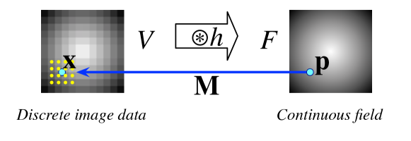
Figure 1: Probing a 2D field $F=h\circledast{}V$ at p, where M is the mapping from world coordinates to image-space coordinates

Handling differentiation of fields requires pushing the differentiation operators down to the convolutions, where they can be applied to the kernel functions. Symbolically, this transformation is

$$\nabla{}F(\mathbf{p})\Rightarrow\nabla{}(H\circledast V)(\mathbf{p})\Rightarrow((\nabla{}H)\circledast V)(\mathbf{p})$$

Because we use separable kernels, their differentiation is straightforward:

$$\nabla H(x,y)=\left[\begin{array}[]{c}\frac{\partial}{\partial_{x}}\\[5.0pt] \frac{\partial}{\partial_{y}}\end{array}\right]H(x,y)=\left[\begin{array}[]{c}\frac{\partial}{\partial_{x}}H(x,y)\\[5.0pt] \frac{\partial}{\partial_{y}}H(x,y)\end{array}\right]=\left[\begin{array}[]{c}\frac{\partial}{\partial_{x}}(h(x)h(y))\\[5.0pt] \frac{\partial}{\partial_{y}}(h(x)h(y))\end{array}\right]=\left[\begin{array}[]{c}h^{\prime}(x)h(y)\\[5.0pt] h(x)h^{\prime}(y)\end{array}\right]$$

where $h^{\prime}$ is the first derivative of $h$.

Thus, the process of implementing a probe operation requires expanding the definition of the field and then normalizing the resulting expression so that code for the appropriate reconstruction can be generated. As we saw above, normalization involves pushing differential operators down to the initial-field definitions. It also involves distributing differential operators and pushing probes down below lifted operators. In effect, part of normalization involves lowering higher-order operators to their first-order equivalents. For example, the probe of the gradient sum of two fields is normalized to the sum of probes of gradients:

$$\nabla(F+G)(x)\Rightarrow(\nabla{}F+\nabla{}G)(x)\Rightarrow\nabla{}F(x)+\nabla{}G(x)$$

which can then be handled as above. The normalization process is a necessary part of the translation of Diderot into executable code.

2.3 Direct vs. index-sensitive operators

We find it is useful to make a distinction between what we call direct-style operators and those that we describe as index-sensitive. This distinction is important for comparing the expressiveness of different implementation approaches, but is not visible in the surface language. Roughly speaking, the mathematical definition of a direct-style operations does not depend on the choice of a coordinate system (e.g., the dot product is mathematically defined in terms of the cosine of the angle between vectors), whereas the definition of index-sensitive operations relies on some choice of coordinate system and the indices into the individual coordinates of quantities expressed in that coordinate system. From the point of view of the implementation, index-sensitive operations require explicit manipulation of indices. A common example of an index-sensitive operation is the curl, which is discussed in Section 4 (see Figure 3).

2.4 Compiler architecture

This paper is, in part, a tale of two compilers: the first Diderot compiler [12], which suffered from various limitations, and the current compiler, which addresses those limitations. Both of these compilers have the same basic architecture, which we describe here.

The Diderot compiler is organized into three main phases: the front-end, optimization and lowering, and code generation. The front-end handles parsing, type checking, and some preliminary optimizations, and produces a simplified monomorphic representation, called Simple AST, where temporaries are introduced for intermediate values and operators are applied only to variables. The middle phase lowers the surface-language operations (e.g., field probes) to low-level code (e.g., memory and arithmetic operations to reconstruct field values). It consists of three stages, where each stage manipulates a different intermediate representation. These IRs share a common Static Single Assignment (SSA) form [15], but different in their types and operations.

HighIR

is essentially a desugared version of the source language with source-level types and operations.

MidIR

supports vectors, transforms between coordinate spaces, loading image data, and kernel evaluations. At this stage, fields and probes have been compiled away into first-order code.

LowIR

supports basic operations on vectors, scalars, and memory objects.

The translations between these representations replaces higher-level operations with their equivalent lower-level operations. For example, field probes in the HighIR (after normalization) are expanded into the convolution of image samples and kernel evaluations in the MidIR. We apply a value-numbering pass to eliminate redundant computation on each of the IRs. For our domain, redundant computations naturally arise in many places; for example, the Hessian produces symmetric matrices and reconstruction of field overlaps with the reconstruction of its gradient. The final phase takes the LowIR representation and converts it to expression trees and statements, which are emitted as vectorized C code and then compiled to either a standalone executable or a library that can be embedded in a larger application.

In this paper, we are primarily interested in the representation of operations in the optimization and lowering phase.

3 Motivation

In programming, as in mathematics, there is a great expressiveness benefit in being able to lift simple operations to work on higher-order values. In Diderot’s domain of image analysis and visualization algorithms, we see this benefit in the lifting of linear-algebra operations (e.g., vector-norm or dot product) to work on tensor fields.

For example, accurate and robust detection of surfaces (or edges) in images is an important part of volume-rendering applications. A classical principle of edge detection proposed by Canny is that edges are where the image gradient magnitude is maximized with respect to motion along the gradient direction [8]. In a scalar tensor field $F$, the locations where $|\nabla F(x)|$ is maximized with respect to motion along $\nabla F(x)/|\nabla F(x)|$ are where $\nabla|\nabla F(x)|$ (the gradient of quantity being maximized) is orthogonal to $\nabla F(x)/|\nabla F(x)|$. In other words, the set of points where the field

$$E=-\nabla|\nabla{}F|\mathbin{\bullet{}}\frac{\nabla{}F}{|\nabla{}F|}$$

is zero (i.e., $E(x)=0$). Notice that the definition of $E$ is higher-order; i.e. it is purely in terms of fields and higher-order operations on fields. We believe that this kind of higher-order notation is the most natural way for an image-analysis expert to reason about and develop image-analysis algorithms.

The first implementation of Diderot [12] had some significant limitations in how well it supported higher-order programming with tensor fields. Specifically, it could not fully support index-sensitive operations, such as the curl on fields ($\nabla{}{\times}$) and it only lifted a very limited set of linear-algebra operations to work on fields (just scalar multiplication, field addition, and field subtraction), which meant that the style of higher-order programming described above was not possible. Instead, it was necessary for a programmer to derive by hand the first-order implementation of the higher-order reasoning. Such a process is time-consuming, error-prone, and can result in a significant increase in the size of the code [10].

The limitations on higher-order operations were owed to the representation of operations in the previous compiler’s IR. As described in Section 2.4, the compiler uses an SSA representation for the optimization and lowering phase. In the previous compiler, we defined a fixed set of direct-style operators, such as DotProduct, FieldAdd, FieldGrad, for the HighIR, which corresponded to the surface-language operators. This representation allowed a straightforward implementation of normalization and other transformations using term rewriting [12]. There was a problem, however, in that adding a single new field-level operator would require adding additional rewrite rules for the possible combinations of that operator and the other field operations, as well as operator-specific lowering code and down-stream support for the operator. Essentially, every lifted operator would be a special case in the IR.

To address these limitations we developed a new intermediate representation, called EIN, for the Diderot compiler. This representation allows a wide range of higher-order computations, including expressions like

⬇

field#2(3)[] E = -$\nabla$(|$\nabla$F|) $\bullet$ $\nabla$F/|$\nabla$F|;

for the edge detection example. The EIN representation has enabled a new level of flexibility and expressiveness in the Diderot language. This expressiveness makes developing sophisticated new algorithms easier, faster, and more intuitive. Diderot programmers are able to express their ideas in a high-level mathematical notation and then rely on the compiler to handle the necessary derivations to realize an implementation. We present two examples of the benefit of this expressiveness in Section 7.

4 The design of EIN

The desire to support higher-order programming with tensor fields required a redesign of the exiting IR. The resulting design needed to satisfy several requirements:

1. it must support the normalization transformations that are needed to turn probes of arbitrary fields into realizable computations;

2. it must provide a mechanism to express index-sensitive operations on fields (e.g., curl); and

3. it must be easily extensible to new operations on both tensors and fields.

The existing direct-style operators in the previous compiler only satisfied the first of these requirements. While it was possible to add operations like curl as IR operators, they would have to be treated as black boxes by the compiler and their use prevents further differentiation of the result. Lastly, adding new operations on field required adding new normalization rewrites for all of the existing field operations, as well as new lowering and code generation code.

An alternative approach that we considered was immediately expanding the tensor structure into loops or unrolled straight-line code in the SSA. This approach has the major drawback that the normalization transformations become more difficult; the cost of normalization is higher, since each component of a field-valued expression is normalized separately, and the size of the IR might explode.

Although there were drawbacks to the previous compiler’s IR; there were positive aspects as well. The SSA-representation provided a good basis for standard compiler analyses and optimizations, such as value numbering. Also direct-style operators abstract away from the implicit iterative structure required to implement them, which helped keep the size of the IR manageable during compilation. Only at the last stage, after much redundancy had been eliminated, did we expand out the iterative code into vectorized operations. In designing a new IR, we wanted to preserve these positive features as much as possible, while adding new flexibility to meet the other design goals. Our solution is to keep the existing SSA representation, but to replace the tensor and tensor-field operators with a family of operators defined by expression trees. We add a new form of SSA operator, called an EIN operator, which has the form $\lambda{}\,\mathit{xs}{\left\langle{e}\right\rangle}_{\sigma}$, where

• $\mathit{xs}\in\textsc{Var}^{*}$ are the parameters of the operator;

• $e$ is an EIN expression that is the body of the operator; and

• $\sigma\in(\textsc{IndexVar}\times\mathbb{N})^{*}$ defines the index space of the operator, where the first component of the pairs are the index variables and the second components are the upper bounds (the lower bounds are $1$ by definition). If $\sigma=i_{1}\leq d_{1},\,\ldots,\,i_{k}\leq d_{n}$, then the shape of the tensor (or tensor field) defined by the operator is $d_{1},\ldots,d_{n}$.

One can think of the index space as defining an $n$-deep loop nest over the index variables where the expression $e$ is the loop body that defines scalar components of the result. The scope of the parameters and index variables is $e$. At the SSA level, these operators are applied to arguments on the right-hand-side of assignments; e.g., $t=\lambda{}\,\mathit{xs}{\left\langle{e}\right\rangle}_{\sigma}(\mathit{ys})$. By keeping the operator definition separate from the arguments, optimizations at the SSA level can analyze and transform these assignments without having to examine the body $e$ of the EIN operator.

$$\begin{array}[]{rclr}\textbf{E}&::=&\lambda{}\,\bar{x}{\left\langle{e}\right\rangle}_{\sigma}&\text{EIN{} Operator}\\[5.0pt] e&::=&T_{\alpha}&\text{Indexed tensor parameter}\\ &\mid&F_{\alpha}&\text{Indexed field parameter}\\ &\mid&\delta_{ij}&\text{Kronecker delta}\\ &\mid&\mathcal{E}_{ij}\;\mid\;\mathcal{E}_{ijk}&\text{Levi-Civita tensor}\\ &\mid&\sin(e)\;\mid\;\arcsin(e)\;\mid\,\ldots\,\mid\;\arctan(e)&\text{Trig.\ functions}\\ &\mid&\sqrt{e}\;\mid\;-e\;\mid\;\exp(e)\;\mid\;e^{n}&\text{Unary operators}\\ &\mid&e+e\;\mid\;e-e\;\mid\;e*e\;\mid\;\frac{e}{e}&\text{Binary operators}\\ &\mid&\sum\limits_{n\leq{}i\leq{}n^{\prime}}e&\text{Summation}\\[2.5pt] &\mid&e_{1}@e_{2}&\text{Probe of a field $e_{1}$ at position $e_{2}$}\\ &\mid&{\textbf{lift}({e})}&\text{Lift tensor $e$ to a field}\\ &\mid&V_{\alpha}\circledast H^{\beta}&\text{Convolution}\\ &\mid&\frac{\partial}{\partial x_{i}}\diamond e&\text{Partial derivative of $e$}\\[5.0pt] \sigma&\in&(\textsc{IndexVar}\times\mathbb{N})^{*}&\text{Index map}\\[5.0pt] i,j,k&\in&\textsc{IndexVar}&\text{Variable index}\\[5.0pt] n&\in&\mathbb{N}&\text{Constant index}\\[5.0pt] \mu&\in&\textsc{Index}=\textsc{IndexVar}\cup\textsc{ConstVar}&\text{Single index}\\[5.0pt] \alpha,\beta,\gamma&\in&\textsc{Index}^{*}&\text{Sequence of indices}\\ \end{array}$$

Figure 2: The syntax of EIN operators and EIN expressions in HighIR

The syntax of EIN operators and expressions is given in Figure 2. An expression can be an indexed tensor ($T_{\alpha}$) or tensor-field ($F_{\alpha}$) parameter ($\alpha$ defines which component of the tensor is referenced). The Kronecker delta and Levi-Civita tensors are used to are used to permute and cancel components based on their indices. EIN expressions also include the trigonometric functions and standard arithmetic operators. The summation expression introduces an additional index variable and is the only binding form in the EIN expressions. We use the syntax $e_{1}@e_{2}$ to represent the probe of a field defined by $e_{1}$ by the value $e_{2}$. The expression $\textbf{lift}({e})$ expression lifts a tensor value to be a constant field. Initial fields are defined by convolution $V_{\alpha}\circledast H^{\beta}$ of an image $V$ with a kernel $H$, where $\alpha$ indexes the shape of voxels in the image (e.g., if $V$ is a vector image, then $\alpha$ will be a single index ranging over the vector indices) and $\beta$ specifies the differentiation of the kernel. Lastly, the application of the partial derivative with respect to the $i$th axis of an expression is represented as $\frac{\partial}{\partial x_{i}}\diamond e$. EIN expressions are also used in the MidIR, but at that point fields have been rewritten to tensor computations and so the syntactic forms for field expressions are not used.

Index maps ($\sigma$) and indices play an important rôle in the syntax and semantics of EIN. Indices can either be variables (denoted by $i$, $j$, and $k$), or constants ($n\in\mathbb{N}$). We use $\alpha$ and $\beta$ to denote sequences of zero or more indices of either type. When describing transformations it will be useful to connect the variables bound in an index map with the indices of a tensor or field variable. We use the notation $\hat{\alpha}$ to denote an index map, where $\alpha$ is the corresponding sequence of index variables.

The EIN representation is a hybrid design that embeds expression trees into a normalized SSA representation. This design preserves the useful properties of the SSA representation, while providing flexibility in the specification of tensor and tensor-field operations. The key property of this design is that it allows reference to indices in the body of $e$ (thus supporting index-sensitive operators), while also providing a compact representation of the nested iteration that is implicit in the definition of tensors and tensor fields.

To give some intuition for EIN operators we present a number of examples of common operators in Figure 3.

$$\begin{array}[]{rcll}\mathbf{u}\bullet{}\mathbf{v}&\equiv&\lambda{}\,U,V{\left\langle{U_{i}*V_{i}}\right\rangle}_{i\leq{}n}(\mathbf{u},\mathbf{v})&\text{{Inner (dot) product of $n$-vectors}}\\[2.5pt] \mathbf{u}\otimes{}\mathbf{v}&\equiv&\lambda{}\,U,V{\left\langle{U_{i}*V_{j}}\right\rangle}_{i\leq{}n,j\leq{}m}(\mathbf{u},\mathbf{v})&\text{{Outer product of vectors}}\\[2.5pt] \mathbf{u}\times{}\mathbf{v}&\equiv&\lambda{}\,U,V{\left\langle{\sum\limits_{j\leq{}3}\sum\limits_{k\leq{}3}\mathcal{E}_{ijk}*U_{j}*V_{k}}\right\rangle}_{i\leq{}3}(\mathbf{u},\mathbf{v})&\text{{Cross product of vectors}}\\[2.5pt] \mathrm{trace}(\mathbf{M})&\equiv&\lambda{}\,T{\left\langle{\sum\limits_{i\leq{}n}T_{i,i}}\right\rangle}(\mathbf{M})&\text{{Trace of an $n\times{}n$ matrix}}\\[2.5pt] \mathbf{M}^{T}&\equiv&\lambda{}\,T{\left\langle{T_{j,i}}\right\rangle}_{i\leq{}n,j\leq{}m}(\mathbf{M})&\text{{Matrix transpose}}\\[2.5pt] \nabla{\times{}}\mathbf{f}&\equiv&\lambda{}\,F{\left\langle{\sum\limits_{j\leq{}3}\sum\limits_{k\leq{}3}\mathcal{E}_{ijk}*\frac{\partial}{\partial x_{j}}\diamond F_{k}}\right\rangle}_{i\leq{}3}(\mathbf{f})&\text{{Curl of a vector field}}\end{array}$$

Figure 3: Examples of common operators encoded as EIN operator applications

The last of these examples, is the curl of a vector field;, which is an example of an index-sensitive operation on fields that was not handled fully in the previous compiler’s IR (satisfying the second of our design goals). In the next section, we describe the compiler transformations that we apply to EIN and show that it satisfies the other two design goals.

5 Implementation

With the design of the EIN IR we had to also develop new techniques for optimization and lowering, which we describe in this section. Switching to EIN in the compiler enabled a new class of program that were not supported by the previous compiler. Unfortunately, it turned out that some of these programs caused an explosion in the size of the EIN IR is our first implementation of it. We describe the techniques for managing the size of the IR during compilation that de developed.

5.1 Translation

The Diderot compiler generates HighIR, including the EIN operators, from the monomorphic Simple AST representation produced by the front end. The translation from the Simple AST to HighIR is aided by the definition of meta-level generic EIN operators that are parameterized over types, shapes, and dimensions. In the Simple AST, surface-language operations have been mapped to monomorphic instances of shape-polymorphic operations. We then can convert Simple AST operations to EIN operators by applying the corresponding generic operator to the type/shape/dimension parameters of the AST operator. This approach allows many similar operations to be defined by a single generic operator. For example, vector-vector, vector-matrix, matrix-vector, and matrix-matrix multiplication are all instances of the same generic inner-product operator. This mechanism also makes it fairly easy to extend the language with new operators.

5.2 Fusion

The result of the translation from Simple AST to High IR is a program where every surface operation is represented by an SSA assignment. To enable transformations of the EIN expressions, we must first fuse operations to produce larger expressions that are amenable to useful transformations. The basic idea is that if we have two SSA assignments involving EIN operators

$$\begin{array}[]{l}t_{1}=\lambda{}\,\mathit{xs}{\left\langle{e_{1}}\right\rangle}_{\sigma_{1}}(\mathit{ys})\\ \cdots\\ t_{2}=\lambda{}\,\ldots,\,t,\,\ldots{\left\langle{e_{2}}\right\rangle}_{\sigma_{2}}(\ldots,\,t_{1},\,\ldots)\end{array}$$

then we want to substitute $e_{1}$ for $t_{1}$ in $e_{2}$, while adding the $\mathit{xs}$ to the parameters of the second operator and the $\mathit{ys}$ to its arguments.

The fusion transformation has the potential to explode the size of the program. In our experience, this problem does not occur for HighIR in real programs, but code duplication does cause problems down stream in Mid and Low IR, as we discuss below.

5.3 Normalization

As explained in Section 2.2, the lowering of HighIR probe operations to reconstruction code requires first normalizing the field definitions that are being probed. We implement this process as a rewriting system on the bodies of EIN operations after fusion.

The basic strategy of normalization is as in the previous compiler: an EIN expression in normal form will have field reconstructions, possibly involving derivatives of the kernels, at the leaves, probe operations at the next level up, and then first-order tensor operations in the levels above. Space does not permit a complete presentation of the rules, but we highlight the key rewrites here. The full system is described in the first-author’s Ph.D. dissertation [10], including a formal definition of the normal form and proofs that the rewrite system terminates, preserves types, and produces terms in normal form.

Pushing probes below lifted operators is the purpose of the following rules. which distribute the probes over unary and binary operations:

$$\begin{array}[]{ccc}(-F_{\alpha})@x\Rightarrow-({F_{\alpha}@x})&&\sqrt{F_{\alpha}}@x\Rightarrow\sqrt{F_{\alpha}@x}\\ \lx@intercol\hfil(e_{1}\odot{}e_{2})@x\Rightarrow(e_{1}@x)\odot{}(e_{2}@x)\quad\text{where $\odot\in\{{+},{-},{*}\}$}\hfil\lx@intercol\end{array}$$

Similar rules existed in the previous compiler, but only for a very limited set of operators.

We also need rules to apply differentiation to other operators and, in this way, push it down toward the leaves. These rules are justified by the semantics of tensor calculus [18]. For example, we have multiple rewrite rules that embody the chain rule from calculus, such as

$$\frac{\partial}{\partial x_{i}}\diamond(\textbf{exp}(e))\Rightarrow\textbf{exp}(e)(\frac{\partial}{\partial x_{i}}\diamond e)$$

and a rewrite for the quotient rule

$$\frac{\partial}{\partial x_{i}}\diamond\frac{e_{1}}{e_{2}}\Rightarrow\frac{(\frac{\partial}{\partial x_{i}}\diamond e_{1})e_{2}-e_{1}(\frac{\partial}{\partial x_{i}}\diamond e_{2})}{e_{2}^{2}}$$

Other rules handle cases such as distribution over binary operators

$$\frac{\partial}{\partial x_{i}}\diamond(e_{1}\odot e_{2})\Rightarrow(\frac{\partial}{\partial x_{i}}\diamond e_{1})\odot(\frac{\partial}{\partial x_{i}}\diamond e_{2})\quad\text{for $\odot\in\{{+},{-}\}$}$$

and trigonometric identities

$$\frac{\partial}{\partial x_{i}}\diamond\arccos(e)\Rightarrow\frac{-(\frac{\partial}{\partial x_{i}}\diamond e)}{\sqrt{(\textbf{lift}({1})-(e*e)}}$$

Once the differenttiation operator is pushed down to an initial-field definition, we rewrite the expression by moving the indices on the differentiation operator to the reconstruction kernel.

$$\frac{\partial}{\partial x_{\mu}}\diamond(V_{\alpha}\circledast H^{\beta})\Rightarrow V_{\alpha}\circledast H^{\beta\mu}$$

5.4 HighIR optimizations

In addition to normalization, we also include a number of domain-specific rewrites the optimize terms in our HighIR rewriting system. An important class of these are index-based reductions that allow us to eliminate summations (i.e., effectively reduce the loop-nesting depth).

$$\sum_{jk}\mathcal{E}_{ijk}\left(\frac{\partial}{\partial x_{ij}}\diamond e\right)\Rightarrow\textbf{lift}({0})$$

Two epsilons in an expression with a shared index can be rewritten to deltas [13].

$$\sum_{i}\mathcal{E}_{ijk}\mathcal{E}_{ilm}\Rightarrow\delta_{jl}\delta_{km}-\delta_{jm}\delta_{kl}$$

Application of a $\delta_{ij}$ to tensors and fields can be simplified.

$$\begin{array}[]{ccccccc}\sum_{j}\delta_{ij}T_{j}\Rightarrow T_{i}&&\sum_{j}\delta_{ij}F_{j}\Rightarrow T_{i}&&\sum_{j}\frac{\partial}{\partial x_{j}}\diamond\delta_{ij}e\Rightarrow\frac{\partial}{\partial x_{i}}\diamond e\end{array}$$

Lastly, we also include rewrites that implement standard constant folding of arithmetic expressions.

One of the nice features of the rewriting system is that “discovers” identities without having to have specific rules. For example, the compiler will reduce the trace of the outer product of two vectors to their dot product, and it will reduce $\nabla\bullet\nabla\times F$ to zero. Another example is the simplification

$$(a\times b)\bullet(c\times d)\Rightarrow(a\bullet c)(b\bullet d)-(a\bullet d)(b\bullet c)$$

(the right-hand side is preferred because it involves fewer arithmetic operations). The EIN operator created for the left-hand side has the body

$$\sum_{i}(\sum_{jk}\mathcal{E}_{ijk}a_{j}b_{k})(\sum_{lm}\mathcal{E}_{ilm}c_{l}d_{m})$$

During normalization the two epsilons with a shared index are reduced to deltas

$$(\sum_{jklm}\delta_{jl}\delta_{km}a_{j}b_{k}c_{l}d_{m})-\sum_{jklm}(\delta_{jm}\delta_{kl}a_{j}b_{k}c_{l}d_{m})$$

The deltas reduction produces

$$(\sum_{jk}a_{j}b_{k}c_{j}d_{k})-\sum_{jk}(a_{j}b_{k}c_{k}d_{j}).$$

The summation binding method (discussed later in this section) produces

$$(\sum_{j}a_{j}c_{j})(\sum_{k}b_{k}d_{k})-(\sum_{j}a_{j}d_{j})(\sum_{k}b_{k}c_{k})$$

which is the EIN representation of $(a\bullet c)(b\bullet d)-(a\bullet d)(b\bullet c)$.

5.5 Lowering to MidIR

Once we have normalized the HighIR, we then need to lower the representation to MidIR. Like HighIR, the MidIR also uses EIN operators as a compact representation of loops over tensor indices After normalization, definitional field expressions are no longer necessary and can be eliminated. Normalization also has the effect of removing the differential operator from the EIN expressions. Thus the resulting MidIR representation involves computations on scalars and tensors, but not fields.

5.6 Lowering to LowIR

In the Mid-IR phase of the compiler, operations between tensors, images, and kernels are represented by EIN operators. The translation to LowIR expands the bodies of the EIN operators into vectorized code. The inner iteration of an operator is usually mapped onto vector operations while any outer iterations are unrolled into straight-line code. Aggressive loop unrolling makes sense in our domain because the number of iterations is typically two or three and the loop-nesting depth is usually one or two.

The LowIR assumes arbitrarily-wide vector operations; these are then mapped onto the available hardware resources (i.e., 128, 256, or 512-bit wide vectors depending on the target machine) as part of the translation to expression trees in the back end.

5.7 Managing the size of the IR

The initial implementation of EIN was found to support the existing body of Diderot programs and benchmarks well with slight improvements in efficiency [9]. There was an unexpected consequence, however from the switch to EIN. With EIN in place, we were able to greatly increase the expressiveness of the Diderot language (by adding more differentiation operators and lifting tensor operations), which in turn enabled richer and more sophisticated Diderot programs. These new programs, which could never have been written in the previous version of Diderot, stressed the compiler in unexpected ways that resulted in lengthy compile times and failures to compile.

In hindsight, the cause of the problem was obvious. The use of fusion on HighIR is necessary to group expressions so that we can effectively apply normalization and lowering. But as noted above, however, it has the effect of duplicating code. In the High and Mid IRs, this code duplication is not a serious problem, but when we lower MidIR to LowIR the duplicated terms get expanded and we get exponential code blowup in some cases. To address this problem, we developed several transformations that we apply to the MidIR immediately after lowering from HighIR. The goal of these transforms is break apart larger EIN operators into smaller ones, where the SSA value-numbering optimization will then be able to eliminate many of them as redundant.

5.7.1 Split

The Split transformation decomposes a large EIN operator into smaller and simpler ones — in some respects, it is the inverse of fusion. The basic idea of Split is fairly simple, but the tricky part is correctly tracking the indices so that we preserve the semantics of the expression. We define the shape of an EIN expression $e$ to be the ordered list of index variables that are free in $e$; these variables are bound in an outer context (either an outer summation or the index map of the containing operator) and the order is given by a top-down, left-to-right ordering of their binding sites [10]. For example, the shape of the expression $T_{j,i}$ in the context $\lambda{}\,\mathit{xs}{\left\langle{\cdot}\right\rangle}_{i\leq{}n_{1},j\leq{}n_{2}}$ is $i\leq{}n_{1},j\leq{}n_{2}$, while the shape of the expression $\sum_{k\leq{}n_{3}}T_{i,k}$ in the same context is just $i\leq{}n_{1}$.

By splitting large EIN operators into smaller ones, it provides opportunities for the value-numbering pass to eliminate redundancy. For example, the subexpression $e$ is embedded inside a larger EIN operator that can be split apart

$$t_{2}=\lambda{}\,A,B{\left\langle{\left(\sum\limits_{\sigma_{1}}e\right)\odot e^{\prime}}\right\rangle}_{\sigma_{2}}(a,b,\ldots)\Rightarrow\begin{array}[]{l}t_{1}=\lambda{}\,B{\left\langle{e}\right\rangle}_{\sigma^{\prime}}(b)\\ t_{2}=\lambda{}\,A,T{\left\langle{\left(\sum\limits_{\sigma_{1}}T_{\alpha}\right)\odot e^{\prime}}\right\rangle}_{\sigma_{2}}(a,t_{1})\end{array}$$

This transformation pulls the inner expression $e$ out to be its own operator where $\sigma^{\prime}$ is the shape of $e$. In the original expression the expression $e$ is replaced by the tensor parameter $T_{\alpha}$ and $\alpha$ correspond to the index variables in $\sigma^{\prime}$. The parameter $B$ occurs in e and is moves to EIN operator $t_{1}$, but $A$ does not and stays with EIN operator $t_{2}$.

5.7.2 Slice

A sliced field is a field term that has at least one constant index ($c$) to indicate a field component. Different sliced field terms are distinct (i.e., $F_{01}\neq{}F_{11}$), but since they depend on the same source data they will generate many of the same base computations. To avoid this redundancy, we decompose an EIN operator with a sliced field term into a structure that is more general, but still applies the necessary tensor slicing operator. With this approach we can capture common terms before translating to lower-level constructs while still maintaining the mathematical meaning behind the original terms. The decomposition is as follows:

$$g=\lambda{}\,F,x{\left\langle{\frac{\partial}{\partial x_{\beta}}\diamond F_{c\alpha}(x)}\right\rangle}_{\hat{\alpha}\hat{\beta}}(f,x)\Rightarrow\begin{array}[]{l}t=\lambda{}\,F,x{\left\langle{\frac{\partial}{\partial x_{\beta}}\diamond F_{\gamma}(x)}\right\rangle}_{\hat{\gamma}\hat{\beta}}(f,x)\\ g=\lambda{}\,T{\left\langle{T_{c\alpha\beta}}\right\rangle}_{\hat{\alpha}\hat{\beta}}(t)\end{array}$$

where $\hat{\gamma}=i\leq{}n,\hat{\alpha}$, the field variable $F$ has type field#k(d)[$n::\varsigma$], and the tensor $x$ has type tensor[d]. The result is a pair of EIN operators: an unsliced field probe and a tensor-valued EIN operator. The defintion of $g$ captures the components of the probe that are of interest. Like, the split method, the slice method creates a representation that will produce a smaller number of lower level constructs.

5.7.3 Summation Binding

Each summation operator represents a loop nest that will be unrolled when lowered to LowIR. Thus moving operations outside the summation can avoid subsequent code duplication. This transformation is essentially loop-invariant code hoisting for the special case of summations. We identify loop invariants by looking at the indices. For example, consider the term $\sum\limits_{\sigma}(T_{\alpha}*e)$ if the property $\forall i\in\alpha.i\not\in\sigma$ holds then we know that $T_{\alpha}$ is invariant and can be lifted.

$$\sum\limits_{\sigma}(T_{\alpha}*e)\Rightarrow T_{\alpha}*\sum\limits_{\sigma}(e)$$

When there are nested summations, then the method applies additional analysis to see if the summation can be converted into the product of independent summations as demonstrated in the example in Section 5.4.

5.7.4 Measuring Size Reduction

The techniques described in this section were motivated by a need to manage the size of the IR during compilation. To evaluate the effectiveness of the techniques, we instrumented the compiler with code to measure the size of the IR at six different points in the compilation pipeline. Figure 4 plots the IR sizes for the program “rsvr,” which is a Diderot program that computes ridge surfaces using higher-order programming. The first thing to note is that the program only compiles if all the optimizations are enabled. The other thing to note is that the size problems are localized to the LowIR following lowering from MidIR. Measurements of other higher-order programs produce similar results. Thus our strategy of applying transforms to the MidIR and then applying value numbering reduces the growth in the IR to a manageable level.

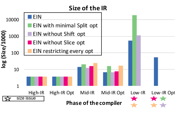
Figure 4: The graphs shows the size of the intermediate representation at different points in the compilation of the the rsvr program. The size is measured by counting the number of expression-tree nodes used to represent the program. “EIN” is the baseline with full optimizations.

6 Benchmarks

While it is clear that the EIN supports a more expressive programming model than the previous compiler, there is still an open question of what effect it has on both compile times and run times. We are also interested in the measured effect of the various transformations described in Section 5.7. To evaluate the impact and cost of the compilation techniques we measure the compilation and execution time for various benchmarks. For the benchmarks we use a mix of Diderot programs with varying degrees of tensor math. We present the results of three experiments: the first compares the performance of EIN with the previous compiler; the second measures the impact of different compiler settings; and the third compares higher-order programs with their first-order equivalents.

6.1 Experimental Framework

The benchmarks were run on an Apple iMac with a 2.7 GHz Intel core i5 processor, 8GB memory, and OS X Yosemite (10.10.5) operating system. Each benchmark was run 10 times and we report the average time in seconds.

The benchmarks are presented in the figures in order of increasing mathematical complexity. Some of the visualization concepts that inspired the benchmarks are described in Section 7. Benchmarks “illust-vr,” “lic2d,” “Mandelbrot,”“ridge3d,” and “vr-lite-cam” are small examples that were used to evaluate the previous compiler [12]. The benchmarks “mode,” “canny,” and “moe” are more sophisticated and were described in a previous paper [28]. “Mode” finds lines of degeneracy in a stress tensor field revealed by volume rendering isosurface of tensor mode; “Canny-edges” computes Canny Edges; and “Moe” volume renders isocontours found using Canny Edges [8].

The benchmarks “dec-crest,” “dec-grad,” “rsvr,” and “mode-rig” have not been featured in previous work because they were not expressible in previous versions of the compiler. The programs “dec-crest” and “dec-grad” are approximations to illustrate the crest lines on a dodecahedron. Programs “mode-rig” and “rsvr” are both programs created to measure ridge lines. The micro-benchmarks “det-grad,”“det-hess,” and “det-trig” compute a single property: the gradient, hessian, and various functions computed on the determinant of a field. Unlike the other benchmarks, these programs are not visualization programs and have negligible runtimes, which we omit.

6.2 Comparing compilers

Our experiments consist of eighteen benchmarks run on three versions of the compiler. The first is the original direct-style compiler [12]. The second and third include the design and implementation techniques included in this paper, but the second version imposes restrictions that are meant to reflect the first naïve implementation of EIN. We measure the time it takes for the programs to compile. For the programs that compile on at least two versions, we also compared the run times. The results are given in Figure 5.

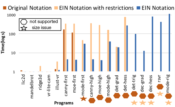
Compile times

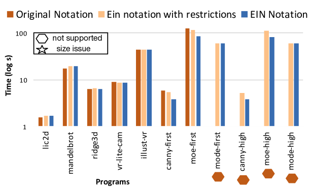
Execution Times

Figure 5: Comparing three different compilers. The “Original”version of the compiler does not use the EIN IR. “EIN with restrictions” is the more naive implementation of EIN. “EIN” is the baseline with the EIN IR with full optimizations applied. Fully implementing EIN allows more programs to compile than previously possible.

We use a hexagon to indicate that the compiler did not support the features used by a program and we use a star symbol to indicate a program that did not compile; the symbols are color coded by compiler.

Not surprisingly, the original compiler was not able to compile many of the programs because of expressiveness issues. And for those that it could compile, its compile times were often significantly slower than EIN. The restricted form of EIN was uniformly worse than EIN in compile times and could not compile the most complex examples. It should be noted, however, that some of the more advanced programs took close to 20 minutes to compile in EIN, so there is room for improvement. The execution-time story is more balanced. The original compiler produces slightly faster code for some benchmarks, but the EIN compiler produced the fastest code for the more complex programs. These results suggest that we have not lost performance by switching to the more expressive IR.

6.3 The Effect of compiler settings

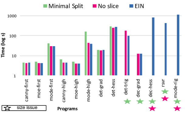
Compile times

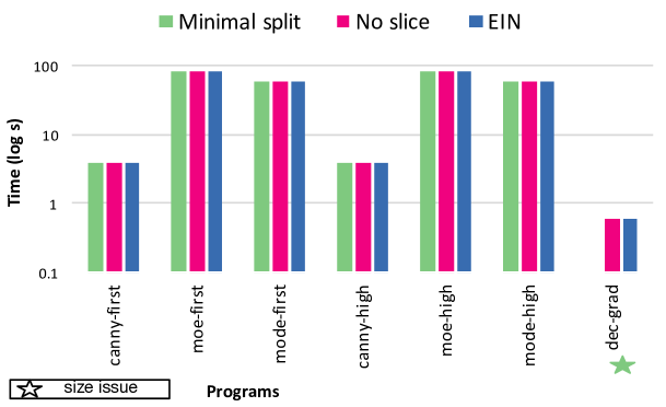
Execution Times

Figure 6: Compile and run time measurements when implementing Slice and Split on High-IR. Doing no amount of splitting prevents most of these programs from compiling so instead we measure its impact by limiting it, “Minimal Split”. EIN is the baseline with both Split and Slice enabled.

As we have discussed previously, a naïve application of our transformations causes unacceptable space blowup. To address the space problem we developed techniques to reduce the size of the IR resulting from lowering passes. While their implementation might allow more complicated Diderot programs to be compiled, we want to evaluate their cost and benefit for programs that could already compile. In the following, we evaluate the effectiveness of these techniques together and isolated at different steps in the compiler.

Application to higher-order constructs

Techniques Split and Slice are effective at reducing the size of the program by finding common subexpressions or reducing field terms. Figure 6 measures the effectiveness of applying Split and Slice on a HighIR EIN operator. The Slice technique is necessary to compile three of the thirteen benchmarks. Split is the most consequential technique. Limiting the application of the method stops five of the programs from being able to compile. Techniques Split and Slice do not add take a considerably longer time to run.

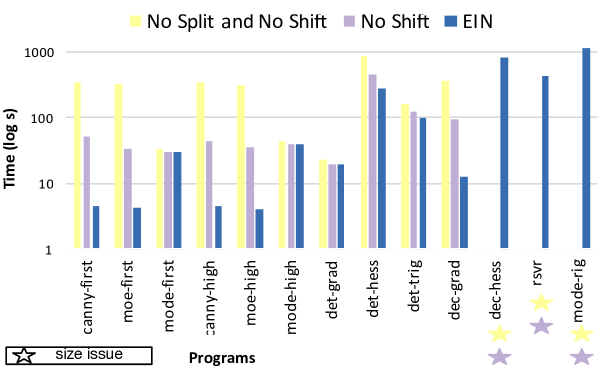
Compile times

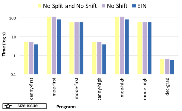
Execution Times

Figure 7: Compile and run time measurements for implementing Shift and Split techniques on reconstructed field terms. EIN baseline includes the application of both Shift and Split.

Application to lower-order constructs

We measured the effect of optimizations at a later phase of the compiler. The implementation of the techniques directly affect compile time. Applying optimizations Shift and Split together offers a consistent speed-up on the execution time and compile time for all thirteen benchmarks. Five programs experienced at least a 20-times improvement in compile time speed-up and four of the benchmarks offered at least a 1.3 speed up on execution time while the rest saw no change in the execution time.

6.4 Higher-order versus first-order programs

For this experiment we wrote both a higher-order and first-order version of three programs. The higher-order programs use lifted tensor operators on fields, whereas the first-order versions only applies tensor operators to tensors. Table 1 gives a breakdown of the relative program sizes in lines of code and Figure 8 shows the compilation and execution times for the two versions. For the first-order version, we measured the performance with both the previous compiler and with EIN.

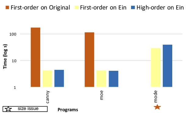
Compile times

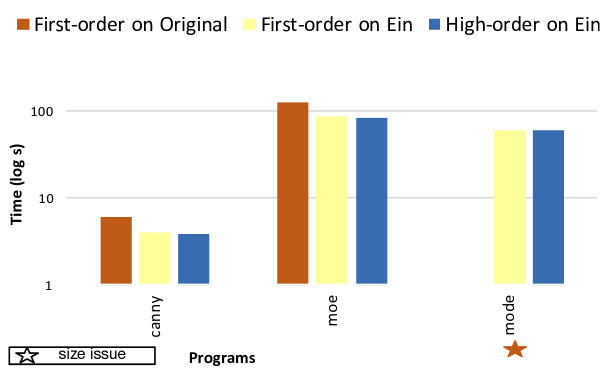
Execution Times

Figure 8: A comparison of hand-derived first-order programs with their higher-order equivalent. The original compiler can only compile the first-order versions, while the compiler with EIN can compile both versions.

The results demonstrate that using higher-order operators in Diderot does not impose a performance penalty in either compile time or execution time. (the one exception was the first-order “mode” program, which compiled slightly faster than the higher-order program).

Table 1: The table reports the lines of code written in a program. Two version of the program are written; “FO” first-order and ‘HO” high-order. The full length of the program is reported as well as the core parts of the program. The table also measures the number of lines used in the field definitions, function declarations, and the central update method.

	Program length		Field Definitions		Functions		Update Method
Program name	FO	HO	FO	HO	FO	HO	FO	HO
Mode	125	75	3	4	19	3	61	25
Moe	84	76	5	4	4	3	29	23
Canny	77	77	2	5	2	2	26	23

7 Applications

Scientists use image analysis to extract features that allow better understanding of their image data. These features can be based on individual pixels, detection of regions with specific shape, time, and transformations of the data [7]. Our work in the EIN IR makes it easier to develop analysis algorithms that exploit higher-order operations. This section describes two visualization techniques [28, 11] that illustrate the effect of switching to the EIN IR in the compiler.

Vector fields arise in the analysis of fluid flow; properties of the derivatives of the vector field characterize important features (such as vortices) in the flow. For example, the curl $\nabla\times V$, indicates the axis direction and magnitude of local rotation. One definition of vortices identifies them with places where the flow direction $\frac{\mathbf{V}}{|\mathbf{V}|}$ aligns with the curl direction $\frac{\nabla\times\mathbf{V}}{|\nabla\times\mathbf{V}|}$ [16]. Normalized helicity measures the angle between these directions:

⬇

field#3(3)[]H = (V/|V|) $\bullet$ ($\nabla\times$V/|$\nabla\times$V|);

in terms of the vector field V. The EIN IR allows the core computation to be expressed directly as operations on fields.

Material properties, such as diffusivity and conductivity, vary locally in magnitude, orientation, and directional sensitivity, so they are modeled with second-order tensor fields. Visualizing the structure of tensor fields typically depends on measuring various tensor invariants, such as anisotropy: the magnitude of directional dependence. For example, neuroscientists study the architecture of human brain white matter with diffusion tensor fields computed from MRI [6]. A popular measure of diffusion anisotropy, “fractional anisotropy” can be directly expressed in Diderot as:

⬇

field#4(3)[3,3]E = T - trace(T)*identity[T]/3;

field#4(3)[]A = sqrt(3.0/2.0)*|E|/|T|

This code measures the magnitude of the purely anisotropic deviatoric tensor relative to the tensor field T itself.

Subsequent visualization or analysis will typically require differentiation, such as the first derivatives needed for shading renderings of isocontours, or the second derivatives needed for extracting ridge and valley features. Generating expressions for $\nabla$ H, and $\nabla$ A by hand is cumbersome and error-prone, whereas EIN allows Diderot to easily handle these and more.

8 Related Work

8.1 Einstein Index Notation

EIN is inspired byEinstein Index Notation, which is a concise written notation for tensor calculus invented by Albert Einstein [20]. Einstein Index Notation uses repeated indices to represent implicit summations (thus it is sometimes called the summation convention). It has be used to represent a wide array of physical quantities and algorithms in scientific computing [1, 5, 13, 18, 35, 36].

Various designers have studied the ambiguities and limitations of the notation to extend its uses on paper and to develop a grammar and semantics for implementation. A part of the ambiguity in index notation is related to the implicit summation. Therefore, various notational definitions are created to suppress summation [1]. These include using notation to differentiate between types of indices, using a no-sum operator [5], and differentiate between indices that repeat exactly twice [18, 36]. EIN notation is a compiler IR so the goal is for the IR to supply enough information to represent the wide range of operations. EIN notation uses an explicit summation symbol so it can explicitly set boundaries for diverse operations. The notation leads to more book-keeping but allows more expressivity.

There is existing work on implementing index notation in a surface language. Ahlander describes supporting index notation for C++ [1] and Egi supports adding index notation to a functional programming language [19].

Ongoing work to implement EIN on the surface level of Diderot is described in the first author’s dissertation [10]. Being able to support an index-like notation directly in Diderot could be beneficial to quick prototyping and debugging. Writing directly in index notation allows the developer to specify computations that may be difficult to replicate with existing surface level operators. It could also help a developer create intricate test cases to more rigorously test the compiler implementation.

8.2 Intermediate representations and optimizations

Domain-specific languages can offer several benefits; the syntax and type system can be designed to meet the practice and expectation of domain experts; the compiler can leverage common domain-specific traits; and the programming model can abstract away from hardware and operating system features. By using a domain specific language, the end-user can write code that is familiar (to them) and let the system focus on generating high-performance code. This notion of developing a high-level mathematical programming model is also emphasized in Diderot. There are various domain-specific languages that provide a link between mathematical algorithms and programming. This section focuses on five domain-specific compilers that are more closely related to our work (Spiral [34], TCE [29], TSFC [27], COFFEE [30], and UFL [2]).

The tensor contraction engine (TCE) created by Hartono, Albert et al. supports a high-level Mathematica style language for the quantum chemistry domain [14, 25, 29]. The class of computations are multi-dimensional summations over products of several arrays. The computations have a large number of nested loops and an explosively large parameter search space. The calculations can require a larger space than available physical memory. To address this issue, Hartono et al. developed algebraic transformations to reduce operation counts. Like TCE, the Diderot language supports summations of products over several arrays. Unlike TCE, Diderot supports a high level of expressiveness between tensors and tensor fields and field differentiation.

Spiral is a DSL created for digital signal processing [22, 32, 34]. Its design encapsulates significant mathematical knowledge of algorithms used in digital signal processing. Püschell et al. addresses the goal of doing the right transformation at the right level of abstraction. Its implementation uses three levels of IR: ${SPL}$ to represent the signal processing language, $\Sigma{SPL}$ to express loops and index mapping, and C-IR for code level optimization. $\Sigma SPL$ does loop merging and create complicated terms that are simplified with a set of rewriting rules [23]. EIN and $\Sigma\text{SPL}$ both use summation expressions to represent loops, but the Spiral IR expresses algorithms, while the EIN IR expresses general tensor calculus. As with Spiral, Diderot allows its users to focus more on the mathematics and allows the system to generate high-performance code for their platform. Although Spiral provides a powerful mathematical model, it is targeted at a somewhat different domain of signal processing.

The Unified Form Language (UFL) is a domain-specific language for representing weak formulations of partial differential equations [2]. UFL is most closely similar to EIN. At its core both UFL and EIN support tensor algebra, high-level expressions with domain-driven abstraction, and offer differentiation (automated vs. symbolic). The projects address different domains, UFL is a language for expressing variational statements of PDEs and Diderot is a language for scientific visualization and image analysis. UFL creates an abstract representation that is used by several form compilers to generate low-level code. Therefore, UFL avoids optimizations that a form compiler might want to perform and instead sticks to a set of “safe and local” simplifications. Diderot controls the entire pipeline from surface language to code generation and so it does have the opportunity to do optimal rewriting at a higher level.

TSFC [27] is a form compiler that takes input from UFL. The TSFC compiler uses an intermediate representation, called GEM. Like EIN, GEM has a notation to represent index summation and tensor components. GEM does not represent the rich range of tensor and field operators, that EIN does. Part of the reason, is because the symbolic differentiation and necessary rewriting is done by UFL and as input TSFC sees a DAG. Diderot maintains the tensor structure for as long as possible. Diderot maps surface level operators directly into EIN notation and in that IR applies rewrites and optimizations.

COFFEE is a domain-specific compiler for local assembly kernels[30]. The computation made by COFFEE is key to finding numerical solutions to partial differential equations. COFFEE computes the contribution of a single cell in a discretized domain for a linear system to approximate a PDE. The entire computation is discretized into a larger number of cells, making the time to compute this computation important. To enable better performance COFFEE applies optimizations. COFFEE applies optimizations on a scalarized tensor expression tree. Like COFFEE, EIN does loop-invariant code motion and expression splitting on tensor expressions. Unlike COFFEE, EIN applies optimizations at a high level to exploit the mathematical properties of the computations on higher-order tensors before flattening

There is extensive work on languages, libraries, and tools focused on efficient execution of math operators. Basic Linear Algebra Subprograms (BLAS) [17] and Linear algebra PACKage (LAPACK)[3] are popular high performance linear algebra libraries. Build to order (BTO) specializes on matrix algebra [31]. FLAME implements linear algebra algorithms and methods in the sequential world [26]. FGen focused on high performance convolution operators or finite-impulse-response (FIR) filters [38]. LGen is a compiler to translate small-scale basic linear algebra expressions to C functions [37]. Like the previous work, Diderot generates code for first-order math operators on tensors. Unlike the previous work, Diderot focuses on higher-order operators, such as differentiation on continuous tensor fields. Also, the tensors in our domain are small vectors and matrices. In the future, our goal is to better leverage the tensor structure to generate faster code.

9 Conclusion

In this paper we have described a new IR that is used in the Diderot compiler. This IR allows us to support a much richer level of mathematical abstraction than was previously possible. The key idea is to use a hybrid approach to the IR design; combining the advantages of a normalized representation (SSA) with a compact representation of loop nests based on expression trees. We have motivated and described our approach and have presented performance results as well as given examples of its utility.

While the techniques that we describe are implemented in the Diderot compiler, we believe that they could be useful for implementing other DSLs that support high-level mathematical programming models.

References

- [1] Ahlander, K.: Einstein summation for multi-dimensional arrays. Computers and Mathematics with Applications 44, 1007–1017 (October – November 2002)
- [2] Alnaes, M.S., Logg, A., Oelgaard, K.B., Rognes, M.E., Wells, G.N.: Unified form language: A domain-specific language for weak formulations of partial differential equations. ACM Trans. Math. Software 40 (Feb 2014)
- [3] Anderson, E., Bai, Z., Dongarra, J., Greenbaum, A., McKenney, A., Du Croz, J., Hammarling, S., Demmel, J., Bischof, C., Sorensen, D.: Lapack: A portable linear algebra library for high-performance computers. In: Proceedings of the 1990 ACM/IEEE Conference on Supercomputing. pp. 2–11. Supercomputing ’90, IEEE Computer Society Press, Los Alamitos, CA, USA (1990), http://dl.acm.org/citation.cfm?id=110382.110385
- [4] Appel, A.W.: Compiling with Continuations. Cambridge University Press, Cambridge, England (1992)
- [5] Barr, A.H.: The Einstein summation notation, introduction to Cartesian tensors and extensions to the notation, draft paper; available from http://citeseerx.ist.psu.edu/viewdoc/summary?doi=10.1.1.118.1377
- [6] Basser, P.J., Pierpaoli, C.: Microstructural and physiological features of tissues elucidated by quantitative-diffusion-tensor MRI. Journal of Magnetic Resonance, Series B 111(3), 209–219 (1996)
- [7] Beutel, J., Kundel, H., Metter, R.L.V.: Handbook of Medical Imaging: Medical Image Processing and Analysis. SPIE Press, Bellingham, WA (2000)
- [8] Canny, J.: A computational approach to edge detection. IEEE Transactions on Pattern Analysis and Machine Intelligence 8(6), 679–714 (1986)
- [9] Chiw, C.: Ein Notation in Diderot. Master’s thesis, Dept. of C.S., U. of Chicago, Chicago, IL (Apr 2014)
- [10] Chiw, C.: Implementing mathematical expressiveness in Diderot. Ph.D. thesis, Dept. of C.S., U. of Chicago, Chicago, IL (May 2017)
- [11] Chiw, C., Kindlman, G.L., Reppy, J.: EIN: An intermediate representation for compiling tensor calculus. In: CPC ’19 (Jul 2016), unpublished position paper
- [12] Chiw, C., Kindlmann, G., Reppy, J., Samuels, L., Seltzer, N.: Diderot: A parallel DSL for image analysis and visualization. In: PLDI ’12. pp. 111–120. ACM, New York, NY (Jun 2012)
- [13] Chow, T.L.: Mathematical Methods for Physicists: A Concise Introduction. Cambridge University Press, Cambridge, England (2000)
- [14] Cociorva, D., Wilkins, J., Lam, C., Baumgartner, G., Sadayappan, P., Ramanujam, J.: Loop optimizations for a class of memory-constrained computations. ICS ’01 pp. 103–113 (2001)
- [15] Cytron, R., Ferrante, J., Rosen, B.K., Wegman, M.N., Zadeck, F.K.: Efficiently computing static single assignment form and the control dependence graph. ACM TOPLAS 13(4), 451–490 (Oct 1991)
- [16] Degani, D., Levy, Y., Seginer, A.: Graphical visualization of vortical flows by means of helicity. American Institute of Aeronautics and Astronautics (AIAA) Journal 28, 1347–1352 (Aug 1990)
- [17] Dongarra, J.J., Du Croz, J., Hammarling, S., Duff, I.S.: A set of level 3 basic linear algebra subprograms. ACM Trans. Math. Software 16(1), 1–17 (Mar 1990)
- [18] Dullemond, K., Peeters, K.: Introduction to Tensor Calculus. Kees Dullemond and Kasper Peeters (1991), http://www.ita.uni-heidelberg.de/~dullemond/lectures/tensor/tensor.pdf
- [19] Egi, S.: Scalar and tensor parameters for importing tensor index notation including einstein summation notation. In: SCHEME ’17 (Sep 2017)
- [20] Einstein, A.: The foundation of the general theory of relativity. In: Kox, A.J., Klein, M.J., Schulmann, R. (eds.) The Collected papers of Albert Einstein, vol. 6, pp. 146–200. Princeton University Press, Princeton NJ (1996)
- [21] Flanagan, C., Sabry, A., Duba, B.F., Felleisen, M.: The essence of compiling with continuations. In: PLDI ’93. pp. 237–247. ACM, New York, NY (Jun 1993)
- [22] Franchetti, F., Mesmay, F., McFarlin, D., Püschel, M.: Operator language: A program generation framework for fast kernels. In: IFIP DSL Working Conference. LNCS, vol. 5658, pp. 385–410. Springer-Verlag, New York, NY (2009)
- [23] Franchetti, F., Voronenko, Y., Püschel, M.: Formal loop merging for signal transforms. In: PLDI ’05. pp. 315–326. ACM, New York, NY (Jun 2005)
- [24] Fraser, C.W., Hanson, D.R.: A Retargetable C Compiler: Design and Implementation. Addison-Wesley, Reading, MA (1995)
- [25] Gao, X., Sahoo, S., Lu, Q., Baumgartner, G., Lam, C., Ramanujam, J., Sadayappan, P.: Performance modeling and optimization of parallel out-of-core tensor contractions. In: PPoPP ’05. pp. 266–276. ACM, New York, NY (Jun 2005)
- [26] Gunnels, J.A., Gustavson, F.G., Henry, G.M., van de Geijn, R.A.: Flame: Formal linear algebra methods environment. ACM Trans. Math. Softw. 27(4), 422–455 (Dec 2001)
- [27] Homolya, M., Mitchell, L., Luporini, F., Ham, D.A.: Tsfc: a structure-preserving form compiler. CoRR abs/1705.03667 (2017), http://arxiv.org/abs/1705.03667
- [28] Kindlmann, G., Chiw, C., Seltzer, N., Samuels, L., Reppy, J.: Diderot: a domain-specific language for portable parallel scientific visualization and image analysis. VIS ’15 22(1), 867–876 (Jan 2016)
- [29] Krishnana, S., Krishnamoorthya, S., Baumgartnerb, G., Chi-Chung Lama, J.R., Sadayappana, P., Choppellaa, V.: Efficient synthesis of out-of-core algorithms using a nonlinear optimization solver. JPDC 66, 659–673 (2006)
- [30] Luporini, F., Varbanescu, A., Rathgeber, F., Bercea, G.T., Ramanujam, J., Ham, D., Kelly, P.: Cross-loop optimization of arithmetic intensity for finite element local assembly. ACM TACO 11(4), Article No. 57 (Jan 2015)
- [31] Nelson, T., Belter, G., Siek, J.G., Jessup, E., Norris, B.: Reliable generation of high-performance matrix algebra. ACM Trans. Math. Softw. 41(3), 18:1–18:27 (Jun 2015)
- [32] Ofenbeck, G., Rompf, T., Stojanov, A., Odersky, M., Püschel, M.: Spiral in Scala: Towards the systematic construction of generators for performance libraries. In: GPCE ’13. pp. 125–134. ACM, New York, NY (Oct 2013)
- [33] Peyton Jones, S., Marlow, S.: Secrets of the glasgow haskell compiler inliner. JFP 12(5), 393–434 (Jul 2002)
- [34] Puschel, M., Moura, J., Johnson, J., Padua, D., Veloso, M., Singer, B., Xiong, J., Franchetti, F., Gacic, A., Voronenko, Y., Chen, K., Johnson, R., Rizzolo, N.: SPIRAL: Code generation for DSP transforms. Proc. of the IEEE 93(2), 232–275 (Feb 2005)
- [35] Simmonds, J.: A Brief on Tensor Analysis. Springer-Verlag, New York, NY (1982)
- [36] Sokolinkoff, I.S.: Tensor Analysis. John Wiley and Sons, New York (1960)
- [37] Spampinato, D.G., Püschel, M.: A basic linear algebra compiler. In: CGO ’14. pp. 23–32 (Feb 2014)
- [38] Stojanov, A., Ofenbeck, G., Rompf, T., Püschel, M.: Abstracting vector architectures in library generators: Case study convolution filters. In: Proceedings of ACM SIGPLAN International Workshop on Libraries, Languages, and Compilers for Array Programming. pp. 14:14–14:19. ARRAY’14, ACM, New York, NY (2014)