Deep neural decoders for near term fault-tolerant experiments

Abstract

Finding efficient decoders for quantum error correcting codes adapted to realistic experimental noise in fault-tolerant devices represents a significant challenge. In this paper we introduce several decoding algorithms complemented by deep neural decoders and apply them to analyze several fault-tolerant error correction protocols such as the surface code as well as Steane and Knill error correction. Our methods require no knowledge of the underlying noise model afflicting the quantum device making them appealing for real-world experiments. Our analysis is based on a full circuit-level noise model. It considers both distance-three and five codes, and is performed near the codes pseudo-threshold regime. Training deep neural decoders in low noise rate regimes appears to be a challenging machine learning endeavour. We provide a detailed description of our neural network architectures and training methodology. We then discuss both the advantages and limitations of deep neural decoders. Lastly, we provide a rigorous analysis of the decoding runtime of trained deep neural decoders and compare our methods with anticipated gate times in future quantum devices. Given the broad applications of our decoding schemes, we believe that the methods presented in this paper could have practical applications for near term fault-tolerant experiments.

I Introduction

Recently, significant progress has been made in building small quantum devices with enough qubits allowing them to be potential candidates for several quantum information experiments Intel ; IBM ; Rigetti ; 2017arXiv170906678N . Fault-tolerant quantum computing is one such avenue that has so far had a very limited experimental analysis Vuillot5qubit . Given the sensitivity of quantum devices to noise, quantum error correction will be crucial in building quantum devices capable of reliably performing long quantum computations. However, quantum error correction alone is insufficient for achieving the latter goal. Since gates themselves can introduce additional errors into a quantum system, circuits need to be constructed carefully in order to prevent errors that can be corrected by the code from spreading into uncorrectable errors. Fault-tolerant quantum computing provides methods for constructing circuits and codes that achieves this goal. However this is at the expense of a significant increase in the number of qubits and the space- time overhead of the underlying circuits (although some methods use very few qubits but have a large space-time overhead and vice-versa).

In recent years, several fault-tolerant protocols for both error correction and universal quantum computation have been proposed, each with their own tradeoffs CS96 ; SteaneCSS ; Knill04 ; Knill05 ; FMMC12 ; CR17v1 ; CR17v2 ; CB17 ; KLZ96 ; JL14 ; PR13 ; ADP14 ; Bombin14 ; YTC16 ; Yoder2017surfacecodetwist . One important aspect of quantum error correcting codes is in finding efficient decoders (the ability to identify the most likely errors which are afflicting the system) that can optimally adapt to noise models afflicting quantum systems in realistic experimental settings. Better decoders result in higher thresholds, and can thus tolerate larger noise rates making near term devices more accessible to fault-tolerant experiments. In CWBL16 , a hard decoding algorithm was proposed for optimizing thresholds of concatenated codes afflicted by general Markovian noise channels. In DP16 ; DP18 , tensor network algorithms were used for simulating the surface code and obtaining efficient decoders for general noise features. However, the above schemes are not adapted to fault-tolerant protocols where gate and measurement errors plays a significant role. Furthermore, some knowledge of the noise is required in order for the decoding protocols to achieve good performance. This can be a significant drawback since it is often very difficult to fully characterize the noise in realistic quantum devices.

The above challenges motivate alternative methods for finding efficient decoders which can offer improvements over more standard methods such as minimum weight perfect matching for topological codes Edmonds65 ; FowlerAutotune and message passing for concatenated codes Poulin06 . One interesting idea is using deep neural networks for constructing decoders which are both efficient and can tolerate large noise rates. The hope is that even if the underlying noise model is completely unknown, with enough experimental data, deep neural networks could learn the probability density functions of the different possible errors corresponding to the sequences of measured syndromes. Note that due to measurement and gate errors, it is often necessary to repeat the syndrome measurements in fault-tolerant protocols as will be explained in Section II.

The first work in which machine learning was used for decoding was in a paper by Torlai and Melko TorlaiNeural . In this paper, a Boltzmann machine was trained to correct phase-flip errors of a 2-dimensional toric code. Krastanov and Jiang obtained a neural network decoder applicable to general stabilizer codes and applied it to the 2-D toric code obtaining a higher code-capacity threshold than previous results. Varsamopoulos, Criger and Bertels used a feed-forward neural network to decode the surface code CrigerNN17 . They also applied their decoding scheme to the distance three surface code under a full circuit level noise model. Baireuther, O’Brien, Tarasinski and Beenakker used a recurrent neural network that could be trained with experimental data Baireuther2018machinelearning . They applied their decoding scheme to compare the lifetime of qubits encoded in a distance-three surface code. The analysis was based on a full circuit level noise model, albeit with a modified CNOT gate error model. Breuckmann and Ni BreuckmannNiNeural gave a scalable neural decoder applicable to higher dimensional codes by taking advantage of the fact that these codes have local decoders. To our knowledge, these methods could not be applied to codes of dimensions less than four. Lastly, while preparing the updated version of our manuscript, Maskara, Kubica and Jochym-O’Connor used neural-network decoders to study the code capacity thresholds of color codes TomasColorCodeNeural .

Despite the numerous works in using neural networks for decoding, there are still several open questions that remain:

1. What are the fastest possible decoders that can be achieved using neural networks and how does the decoding time compare to gate times in realistic quantum devices?

2. Can neural networks still offer good performance beyond distance three codes in a full circuit level noise model regime? If so, what are the limitations?

3. How well do neural networks perform near and below typical thresholds of fault-tolerant schemes under full circuit level noise models?

In this paper we aim to address the above questions. We apply a plethora of neural network methods to analyze several fault-tolerant error correction schemes such as the surface code as well as the CNOT-exRec gate using Steane error correction (EC) and Knill-EC, and consider both distance-three and distance-five codes. We chose the CNOT-exRec circuit since (in most cases) it limits the threshold of the underlying code when used with Steane and Knill-EC units AGP06 . Our analysis is done using a full circuit level noise model. Furthermore our methods are designed to work with experimental data; i.e. no knowledge of the underlying noise model is required.

Lastly, we provide a rigorous analysis of the decoding times of the neural network decoders and compare our results with expected gate delays in future superconducting quantum devices. We suspect that even though inference from a trained neural network is a simple procedure comprising only of matrix multiplications and arithmetic operations, state-of-the-art parallel processing and high performance computing techniques would need to be employed in order for the inference to provide a reliable decoder given the anticipated gate times in future quantum devices.

The deep neural decoders (DND) we design in this paper assist a baseline decoder. For the baseline decoders, we will use both lookup table and naive decoding schemes which will be described in Section II. The goal of the deep neural decoder is to determine whether to add logical corrections to the corrections provided by the baseline decoders. Although the lookup table decoder is limited to small codes, the naive decoder can efficiently be implemented for arbitrary distance codes.

We stress that to offer a proper analysis of the performance of neural network decoders, the neural network should be trained for all considered physical error rates. We believe that from an experimental point of view, it is not realistic to apply a network trained for large physical error rates to lower rate noise regimes. The reason is simply that the network will be trained based on the hardware that is provided by the experimentalist. If the experimentalist tunes the device to make it noisier so that fewer non-trivial training samples are provided to the neural network, the decoder could be fine tuned to a different noise model than what was present in the original device. As will be shown, training neural networks at low error rates is a difficult task for machine learning and definitely an interesting challenge.

Our goal has been to compose the paper in such a way that makes it accessible to both the quantum information scientists and machine learning experts. The paper is structured as follows.

In Section II we begin by providing a brief review of stabilizer codes followed by the fault-tolerant error correction criteria used throughout this paper as well as the description of our full circuit level noise model. In Section II.1, we review the rotated surface code and provide a new decoding algorithm that is particularly well adapted for deep neural decoders. In Sections II.2 and II.3, we review the Steane and Knill fault-tolerant error correction methods and give a description of the distance-three and five color codes that will be used in our analysis of Steane and Knill-EC. In Section II.4 we give a description of the naive decoder and in Section II.5 we discuss the decoding complexity of both the lookup table and naive decoders.

Section III focuses on the deep neural decoders constructed, trained and analyzed in this paper. In Section III.1 we give an overview of deep learning by using the application of error decoding as a working example. We introduce three widely used architectures for deep neural networks: (1) simple feedforward networks with fully connected hidden layers, (2) recurrent neural networks, and (3) convolutional neural networks. We introduce hyperparameter tuning as a commonly used technique in machine learning and an important research tool for machine learning experts. In Sections III.2 and III.3 we introduce the deep neural network architectures we designed for decoding the CNOT-exRec circuits in the case of Steane- and Knill-EC, and for multiple rounds of EC in the case of the rotated surface code.

In Section IV we provide our numerical results by simulating the above circuits under a full circuit level depolarizing noise channel, and feeding the results as training and test datasets for various deep neural decoders.

Finally, in Section V we address the question of practical applicability of deep neural decoders in their inference mode for fault-tolerant quantum error correction. We will address several hardware and software considerations and recommend a new development in machine learning known as network quantization as a suitable technology for decoding quantum error correcting codes.

II Fault-tolerant protocols

In this section we will describe the fault-tolerant protocols considered in this paper. The surface code will be described in Section II.1 while Steane and Knill error correction will be described in Sections II.2 and II.3. For each protocol, we will also describe the baseline decoder used prior to implementing a deep neural decoder (DND). Since we are focusing on near term fault-tolerant experiments, we will first describe decoding schemes using lookup tables which can be implemented extremely quickly for small distance codes. In Section IV we will show that the lookup table decoding schemes provide very competitive pseudo-thresholds. With existing computing resources and the code families considered in this paper, the proposed decoders can be used for distances $d\leq 7$. For example, the distance-nine color code would require 8.8 exabytes of memory to store the lookup table. Lastly, in Section II.4 we will describe a naive decoder which is scalable and can be implemented efficiently while achieving competitive logical failure rates when paired with a deep neural decoder.

Before proceeding, and in order to make this paper as self contained as possible, a few definitions are necessary. First, we define the $n$-qubit Pauli group $\mathcal{P}_{n}^{(1)}$ to be group containing $n$-fold tensor products of the identity $I$ and Pauli matrices $X,Y$ and $Z$. The weight of an error $E\in\mathcal{P}_{n}^{(1)}$ ($\text{wt}(E)$) is the number of non-identity Pauli operators in its decomposition. For example, if $E=IXYIZ$, then $\text{wt}(E)=3$.

A $[\![n,k,d]\!]$ quantum error correcting code, which encodes $k$ logical qubits into $n$ physical qubits and can correct $t=\lfloor(d-1)/2\rfloor$ errors, is the image space $C_{q}$ of the injection $\xi:\mathcal{H}_{2}^{k}\to C_{q}\subset\mathcal{H}_{2}^{n}$ where $\mathcal{H}_{2}$ is the two-dimensional Hilbert space. Stabilizer codes are codes $C_{q}$ which form the unique subspace of $\mathcal{H}_{2}^{n}$ fixed by an Abelian stabilizer group $\mathcal{S}\subset\mathcal{P}_{n}^{(1)}$ such that for any $s\in\mathcal{S}$ and any codeword $|c\rangle\in C_{q}$, $s|c\rangle=|c\rangle$. Any $s\in\mathcal{S}$ can be written as $s=g_{1}^{p_{1}}\cdots g_{n-k}^{p_{n-k}}$ where the stabilizer generators $g_{i}$ satisfy $g_{i}^{2}=I$ and mutually commute. Thus $S=\ \langle g_{1},\cdots,g_{n-k}\rangle$. We also define $N(\mathcal{S})$ to be the normalizer of the stabilizer group. Thus any non-trivial logical operator on codewords belongs to $N(\mathcal{S})\setminus\mathcal{S}$. The distance $d$ of a code is the lowest weight operator $P\in N(\mathcal{S})\setminus\mathcal{S}$. For more details on stabilizer codes see Gottesman97 ; Gottesman2010 .

For a given stabilizer group $\mathcal{S}=\ \langle g_{1},\cdots,g_{n-k}\rangle$, we define the error syndrome $s(E)$ of an error $E$ to be a bit string of length $n-k$ where the $i$-th bit is zero if $[E,g_{i}]=0$ and one otherwise. We say operators $E$ and $E^{\prime}$ are logically equivalent, written as $E\sim E^{\prime}$, if and only if $E^{\prime}\propto gE$ for some $g\in\mathcal{S}$.

The goal of an error correction protocol is to find the most likely error $E$ afflicting a system for a given syndrome measurement $s(E)$. However, the gates used to perform a syndrome measurement can introduce more errors into the system. If not treated carefully, errors can spread leading to higher weight errors which are non longer correctable by the code. In order to ensure that correctable errors remain correctable and that logical qubits have longer lifetimes than their un-encoded counterpart (assuming the noise is below some threshold), an error correction protocol needs to be implemented fault-tolerantly. More precisely, an error correction protocol will be called fault-tolerant if the following two conditions are satisfied AGP06 ; Gottesman2010 ; CB17 :

Definition 1 (Fault-tolerant error correction).

For $t=\lfloor(d-1)/2\rfloor$, an error correction protocol using a distance-$d$ stabilizer code $C$ is $t$-fault-tolerant if the following two conditions are satisfied:

1. For an input codeword with error of weight $s_{1}$, if $s_{2}$ faults occur during the protocol with $s_{1}+s_{2}\leq t$, ideally decoding the output state gives the same codeword as ideally decoding the input state.

2. For $s$ faults during the protocol with $s\leq t$, no matter how many errors are present in the input state, the output state differs from a codeword by an error of at most weight $s$.

A few clarifications are necessary. By ideally decoding, we mean performing fault-free error correction. In the second condition of Definition 1, the output state can differ from any codeword by an error of at most weight $s$, not necessarily by the same codeword as the input state. It is shown in AGP06 ; CB17 that both conditions are required to guarantee that errors do not accumulate during multiple error correction rounds and to ensure that error correction extends the lifetime of qubits as long as the noise is below some threshold.

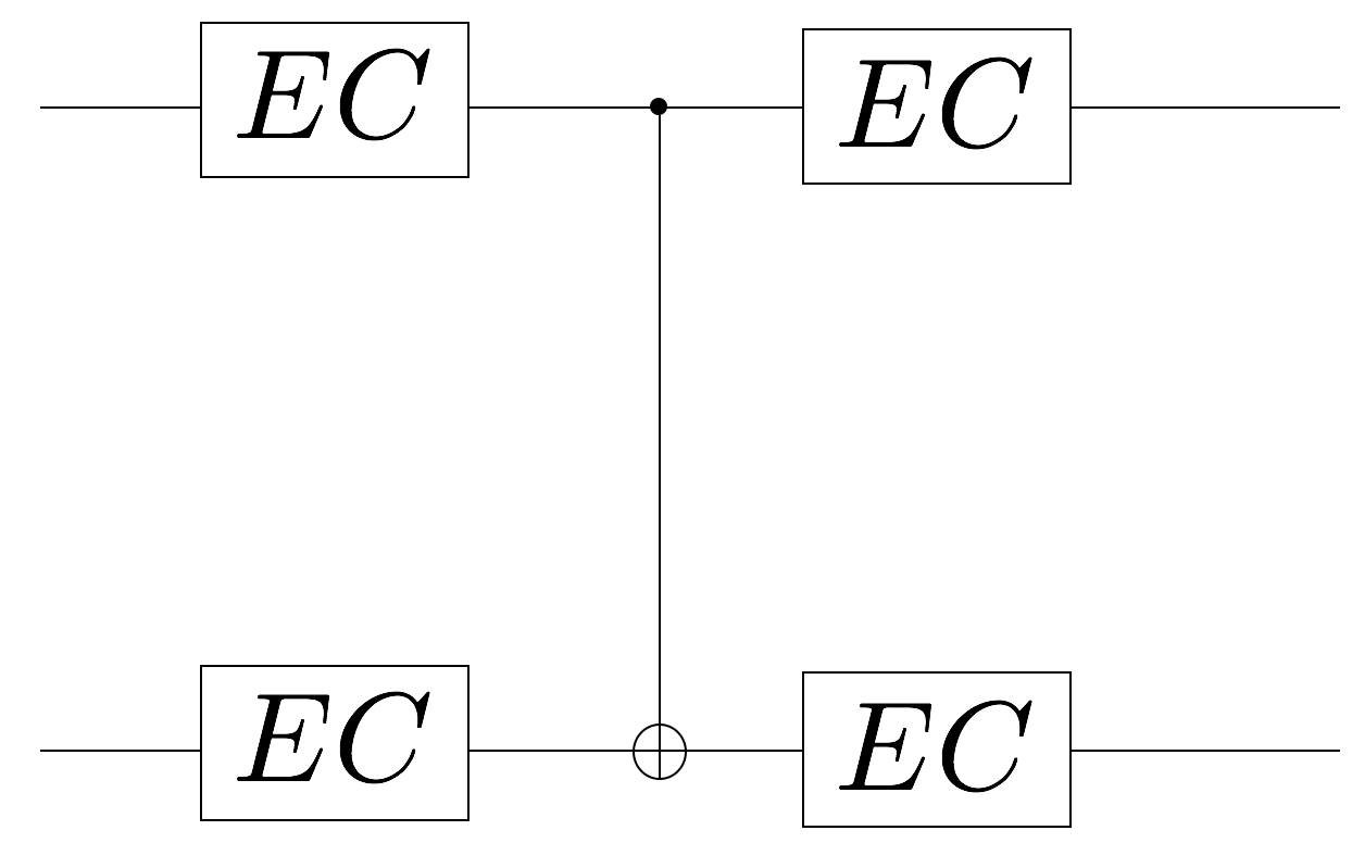
Figure 1: Illustration of an extended rectangle (exRec) for a logical CNOT gate. The EC box consists of performing a round of fault-tolerant error correction. The error correction rounds prior to applying the logical CNOT gate are referred to as leading-EC’s (LEC) and the error correction rounds after the CNOT are referred to as trailing-EC’s (TEC).

In this paper we focus on small distance codes which could potentially be implemented in near term fault-tolerant experiments. When comparing the performance of fault-tolerant error correction protocols, we need to consider a full extended rectangle (exRec) which consists of leading and trailing error correction rounds in between logical gates. Note that this also applies to topological codes. An example of an exRec is given in Fig. 1. We refer the reader to AGP06 ; AGP08 for further details on exRec’s.

In constructing a deep neural decoder for a fault-tolerant error correction protocol, our methods will be devised to work for unknown noise models which would especially be relevant to experimental settings. However, throughout several parts of the paper, we will be benchmarking our trained decoder against a full circuit level depolarizing noise channel since these noise processes can be simulated efficiently by the Gottesman-Knill theorem Gottesman98 . A full circuit level depolarizing noise model is described as follows:

1. With probability $p$, each two-qubit gate is followed by a two-qubit Pauli error drawn uniformly and independently from $\{I,X,Y,Z\}^{\otimes 2}\setminus\{I\otimes I\}$.

2. With probability $\frac{2p}{3}$, the preparation of the $|0\rangle$ state is replaced by $|1\rangle=X|0\rangle$. Similarly, with probability $\frac{2p}{3}$, the preparation of the $|+\rangle$ state is replaced by $|-\rangle=Z|+\rangle$.

3. With probability $\frac{2p}{3}$, any single qubit measurement has its outcome flipped.

4. Lastly, with probability $p$, each resting qubit location is followed by a Pauli error drawn uniformly and independently from $\{X,Y,Z\}$.

II.1 Rotated surface code

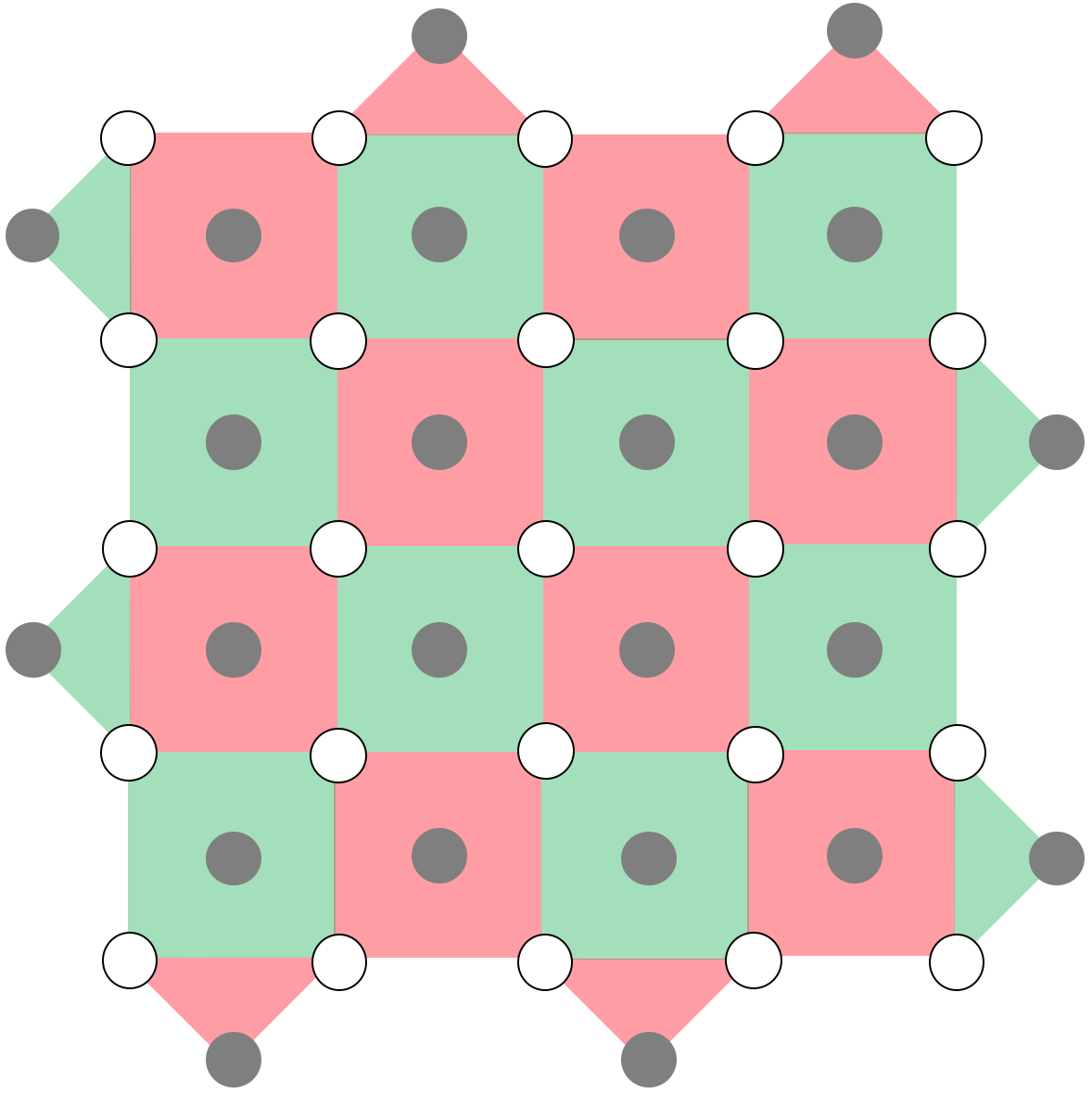
Figure 2: Illustration of the $d=5$ rotated surface code. Data qubits are located at the white circles and the ancilla qubits used to measure the stabilizers are located on the black circles of the lattice. Green squares measure the $Z$ stabilizers and red squares measure $X$ stabilizers.

(a)

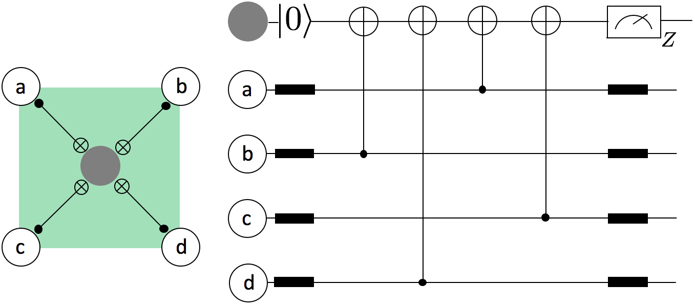
(b)

Figure 3: Fig. 3(a) illustrates the circuit used to measure the stabilizer $X^{\otimes 4}$ and Fig. 3(b) illustrates the circuit used to measure the stabilizer $Z^{\otimes 4}$. As can be seen, a full surface code measurement cycle is implemented in six time steps.

In this section we focus on the rotated surface code BK98 ; DKLP02 ; FMMC12 ; KITAEV97Surface ; TS14 ; PhysRevLett.90.016803 . The rotated surface code is a $[\![d^{2},1,d]\!]$ stabilizer code with qubits arranged on a 2-dimensional lattice as shown in Fig. 2. Any logical $X$ operator has $X$ operators acting on at least $d$ qubits with one $X$ operator in each row of the lattice involving an even number of green faces. Similarly, any logical $Z$ operator has $Z$ operators acting on at least $d$ qubits with one $Z$ operator in every column of the lattice involving an even number of red faces.

It is possible to measure all the stabilizer generators by providing only local interactions between the data qubits and neighbouring ancilla qubits. The circuits used to measure both $X$ and $Z$ stabilizers are shown in Fig. 3. Note that all stabilizer generators have weight two or four regardless of the size of the lattice.

Several decoding protocols have been devised for topological codes. Ideally, we would like decoders which have extremely fast decoding times to prevent errors from accumulating in hardware during the classical processing time while also having very high thresholds. The most common algorithm for decoding topological codes is Edmond’s perfect matching algorithm (PMA) Edmonds65 . Although the best know thresholds for topological codes under circuit level noise have been achieved using a slightly modified version of PMA FowlerAutotune , the decoding algorithm has a worst case complexity of $\mathcal{O}(n^{3})$. Recent progress has shown that minimum weight perfect matching can be performed in $\mathcal{O}(1)$ time on average given constant computing resources per unit area on a 2D quantum computer FowlerO1 . With a single processing element and given $n$ detection events, the runtime can be made $\mathcal{O}(n)$ FowlerSingleProcessor . Renormalization group (RG) decoders have been devised that can achieve $\mathcal{O}(\log{n})$ decoding times under parallelization DuclosRG1 ; DuclosRG2 ; BravyiRG . However such decoders typically have lower thresholds than PMA. Wootton and Loss WootonRG use a Markov chain Monte Carlo method to obtain near optimal code capacity noise thresholds of the surface code at the cost of slower decoding times compared to other schemes. Recently, Delfosse and Nickerson DF17 have devised a near linear time decoder for topological codes that achieves thresholds slightly lower than PMA for the 2-dimensional toric code.

Here we construct a decoder for the surface code which has extremely fast decoding times and achieves high pseudo-thresholds which will serve as a core for our deep neural decoder construction of Section III. Our decoder will be based on a lookup table construction which could be used for distances $d\leq 7$. Before describing the construction of the lookup table, we point out that a single fault on the second or third CNOT gates in Figs. 3(a) and 3(b) can propagate to a data qubit error of weight-two. Thus for a surface code that can correct $t=2d+1$ errors, a correction $E^{\prime}$ for an error $E$ resulting from $t$ faults, with $E^{\prime}\sim E$, must be used when the syndrome $s(E)$ is measured. In other words, the minimum weight correction must not always be used for errors that result from faults occurring at the CNOT gates mentioned above.

With the above in mind, the lookup table is constructed a follows. For every $1\leq m\leq 2^{d^{2}-1}$, use the lowest weight error $E^{\prime}\sim E$ such that converting the bit string $s(E)$ to decimal results in $m$. If $E$ is an error that results from $v\leq t=2d+1$ faults with $\text{wt}(E)>t$, then use $E^{\prime}\sim E$ instead of the lowest weight error corresponding to the syndrome $s(E)$. Note that for this method to work, all errors $E$ with $\text{wt}(E)\leq t$ must have distinct syndromes from errors $E^{\prime}$ that arise from $v\leq t$ faults with $\text{wt}(E^{\prime})>t$. However this will always be the case for surface codes with the CNOT ordering chosen in Fig. 3.

Note that with the above construction, after measuring the syndrome $s$, decoding simply consists of converting $s$ to decimal (say $m$) and correcting by choosing the error on the $m$’th row of the lookup table. Note however that this method is not scalable since the number of syndromes scales exponentially with the code distance.

Lastly, the decoding scheme as currently stated is not fault-tolerant. The reason is that if syndromes are measured only once, in some cases it would be impossible to distinguish data qubit errors from measurement errors. For instance, a measurement error occurring when measuring the green triangle of the upper left corner of Fig. 2 would result in the same syndrome as an $X$ error on the first data qubit. However, with a simple modification, the surface code decoder can be made fault-tolerant. For distance 3 codes, the syndrome is measured three times and we decode using the majority syndrome. If there are no majority syndromes, the syndrome from the last round is used to decode. For instance, suppose that the syndromes $s_{1},s_{2},s_{2}$ were obtained, then the syndrome $s_{2}$ would be used to decode with the lookup table. However if all three syndromes $s_{1},s_{2},s_{3}$ were different, then $s_{3}$ would be used to decode with the lookup table. This decoder was shown to be fault-tolerant in CCBT17 .

For higher distance codes, we use the following scheme. First, we define the counter $n_{\text{diff}}$ (used for keeping track of changes in consecutive syndrome measurements) as

Decoding protocol – update rules: Given a sequence of consecutive syndrome measurement outcomes $s_{k}$ and $s_{k+1}$: 1. If $n_{\text{diff}}$ did not increase in the previous round, and $s_{k}\neq s_{k+1}$, increase $n_{\text{diff}}$ by one.

We also define $E(s)$ to be the correction obtained from either the lookup table decoder or naive decoder (described in section Section II.4) using the syndrome $s$. With the above definition of $n_{\text{diff}}$, the decoding protocol for a code that can correct any error $E$ with $\text{wt}(E)\leq t=\lfloor\frac{(d-1)}{2}\rfloor$ is implemented as

Decoding protocol – corrections: Set $n_{\text{diff}}=0$. Repeat the syndrome measurement. Update $n_{\text{diff}}$ according to the update rule above. 1. If at anytime $n_{\text{diff}}=t$, repeat the syndrome measurement yielding the syndrome $s$. Apply the correction $E(s)$. 2. If the same syndrome $s$ is repeated $t-n_{\text{diff}}+1$ times in a row, apply the correction $E(s)$.

Note that in the above protocol, the number of times the syndrome is repeated is non-deterministic. The minimum number of syndrome measurement repetitions is $t+1$ while in CB17 it was shown that the maximum number of syndrome measurement repetitions is $\frac{1}{2}(t^{2}+3t+2)$. Further, a proof that the above protocol satisfies both fault-tolerance criteria in Definition 1 is given in Appendix A of CB17 .

II.2 Steane error correction

Calderbank-Shor-Steane (CSS) codes CS96 ; SteaneCSS are quantum error correcting codes which are constructed from two classical error correcting codes $C_{1}$ and $C_{2}$ where $C_{1}^{\perp}\subseteq C_{2}$. The last condition guarantees that by choosing the $X$ and $Z$ stabilizers to correspond to the parity check matrices $H_{X}$ and $H_{Z}$ of $C_{1}$ and $C_{2}$, all operators in $H_{X}$ will commute with those of $H_{Z}$. Additionally, CSS codes are the only codes such that a transversal CNOT gate performs a logical CNOT.

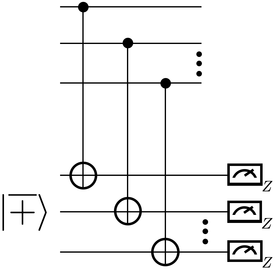
(a)

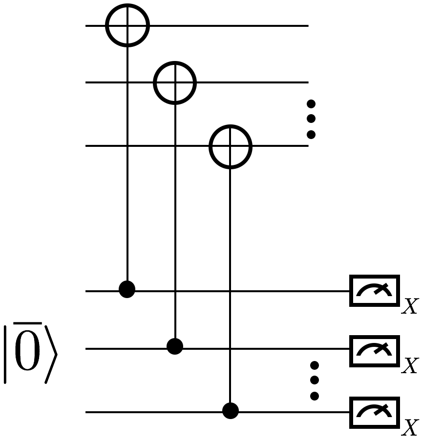
(b)

Figure 4: Circuits for measuring $X$ and $Z$ stabilizers in Steane-EC. The circuit in Fig. 4(a) measures bit-flip errors whereas the circuit in Fig. 4(b) measures phase-flip errors. Note that the first block consists of the data qubits encoded in a CSS code. The states $|\overline{0}\rangle$ and $|\overline{+}\rangle$ represent logical $|0\rangle$ and $|+\rangle$ states encoded in the same CSS code used to protect the data.

Steane error correction Steane97 takes advantage of properties of CSS codes to measure the $X$ and $Z$ stabilizers using transversal CNOT gates. To see this, consider the circuit in Fig. 4(a). The transversal CNOT gate between the encoded data block $|\overline{\psi}\rangle$ and ancilla $|\overline{+}\rangle$ acts trivially (i.e. $\overline{\text{CNOT}}|\overline{\psi}\rangle|\overline{+}\rangle=|\overline{\psi}\rangle|\overline{+}\rangle$). However, any $X$ errors afflicting the data block would then be copied to the ancilla state. Furthermore, CSS codes have the property that transversally measuring the codeword $|\overline{+}\rangle$ in the absence of errors would result in a codeword of $C_{1}$ chosen uniformly at random. If $X$ errors are present on the codeword $|\overline{+}\rangle$, then the transversal measurement would yield the classical codeword $e+f+g$. Here, $(e|0)$ (written in binary symplectic form) are the $X$ errors on the data qubits, $(f|0)$ are the $X$ errors that arise during the preparation of the $|\overline{+}\rangle$ state and $(g|0)$ are bit-flip errors that arise during the transversal measurement. Applying the correction $X_{e}X_{f}X_{g}$ on the data would result in an $X$ error of weight $f+g$. An analogous argument can be made for $Z$ errors using the circuit of Fig. 4(b) (note that in this case we measure in the $X$-basis which maps $C_{1}\rightarrow C_{2}$ and $Z\rightarrow X$).

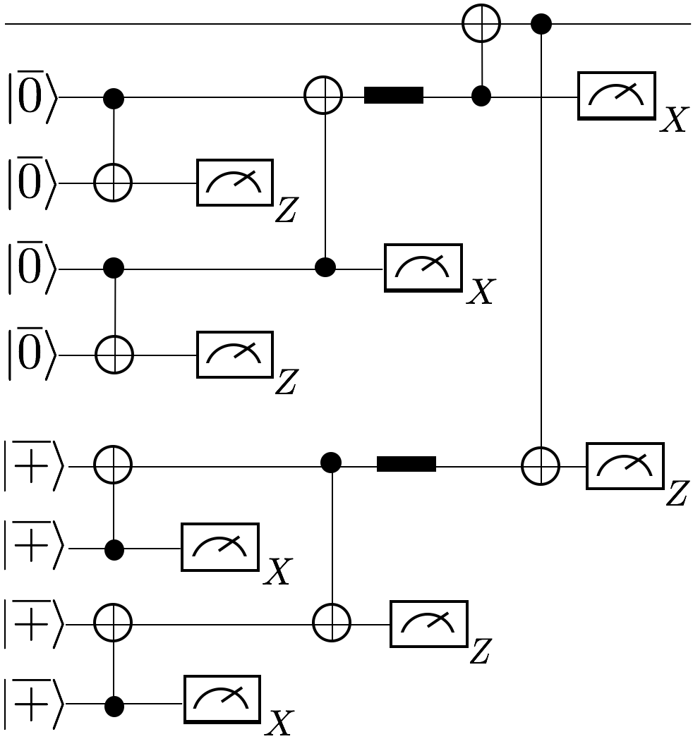
Figure 5: Full Steane error correction circuit. Each line represents encoded data qubits and all CNOT gates and measurements are performed transversally. The circuits used to prepare the encoded $|\overline{+}\rangle$ and $|\overline{0}\rangle$ are in general not fault-tolerant. Consequently, extra ”verifier” ancilla states are used to detect errors arising during the preparation of $|\overline{+}\rangle$ and $|\overline{0}\rangle$. If the verifier states measure a non-trivial syndrome or the $-1$ eigenvalue of a logical Pauli is measured, the ancilla states are rejected and new ancilla states are brought in until they pass the verification step.

Note that the circuits used to prepared the encoded $|\overline{+}\rangle$ and $|\overline{0}\rangle$ states are in general not fault-tolerant. In the case of $|\overline{+}\rangle$, low weight errors can spread to high-weight $X$ errors which can change the outcome of the measurement and $Z$ errors which can propagate to the data block due to the transversal CNOT gates. However, by preparing extra “verifier” states encoded in $|\overline{+}\rangle$ and coupling these states to the original $|\overline{+}\rangle$ ancilla as shown in Fig. 5, high weight $X$ and $Z$ errors arising from the ancilla can be detected. Furthermore, after a classical error correction step, the eigenvalue of $\overline{X}$ and $\overline{Z}$ can be measured. Therefore if a non-trivial syndrome is measured in the verifier states or the $-1$ eigenvalue of a logical operator is measured, the ancilla qubits are rejected and new ancilla qubits are brought in to start the process anew.

We would like to point out that instead of verifying the ancilla qubits for errors and rejecting them when a non-trivial syndrome is measured, it is also possible to replace the verification circuit with a decoding circuit. By performing appropriate measurements on the ancilla qubits and making use of Pauli frames Knill05 ; Barbara15 ; CIP17 , any errors arising from $t$-faults in the ancilla circuits can be identified and corrected DA07 (note that DiVincenzo and Aliferis provided circuits for Steane’s $[\![7,1,3]\!]$ code so that $t=1$). However in this paper we will focus on ancilla verification methods.

It can be shown that the Steane-EC circuit of Fig. 5 satisfies both fault-tolerant conditions of Definition 1 for distance-three codes Gottesman2010 . It is possible to use the same ancilla verification circuits in some circumstances for higher distance codes by carefully choosing different circuits for preparing the logical $|\overline{0}\rangle$ and $|\overline{+}\rangle$ states (see PR12 for some examples). In this paper, we will choose appropriate $|\overline{0}\rangle$ and $|\overline{+}\rangle$ states such that the the decoding schemes will be fault-tolerant using the ancilla verification circuits in Fig. 5. We would like to add that although the order in which transversal measurements to correct bit-flip and phase-flip errors does not affect the fault-tolerant properties of Steane-EC, it does create an asymmetry in the $X$ and $Z$ logical failure rates PR12 ; CJL16 ; CJL16b . For instance, an $X$ error arising on the target qubit of the logical CNOT used to detect phase errors would be copied to the $|\overline{+}\rangle$ ancilla. However a $Z$ error arising on the target of this CNOT or control of the CNOT used to correct bit-flip errors would not be copied to any of the ancilla qubits.

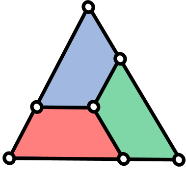
(a)

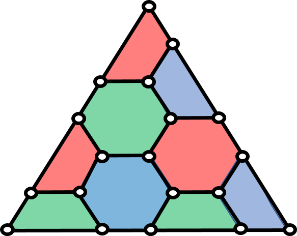
(b)

Figure 6: Fig. 6(a) is a representation of the $[\![7,1,3]\!]$ Steane code. The qubits are located at the white circles of the lattice. Each face corresponds to both a $X^{\otimes 4}$ and $Z^{\otimes 4}$ stabilizer. Fig. 6(b) is a representation of the $[\![19,1,5]\!]$ color code. Like the Steane code, each face corresponds to an $X$ and $Z$ type stabilizer. Notice that there are three weight-six stabilizers of each type.

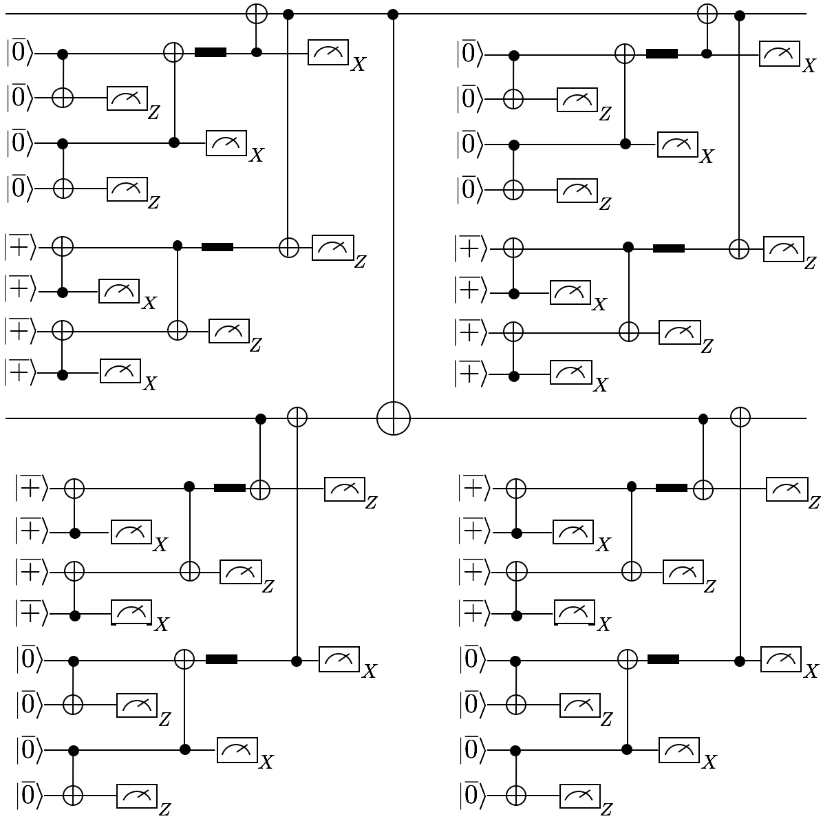
Figure 7: CNOT-exRec for Steane-EC which contains four EC blocks. The CNOT-exRec limits the pseudo-threshold of the $[\![7,1,3]\!]$ and $[\![19,1,5]\!]$ color code due to the large number of locations and thus makes an ideal circuit to optimize our decoding algorithm using machine learning.

We conclude this section by describing the $[\![7,1,3]\!]$ and $[\![19,1,5]\!]$ CSS color codes Bombin06TopQuantDist which will be the codes used for optimizing our decoding algorithms with machine learning applied to Steane and Knill error correction (see Section II.3 for a description of Knill- EC). A pictorial representation for both of these codes is shown in Fig. 6. Both the Steane code and the 19-qubit color code are self-dual CSS codes (meaning that the $X$ and $Z$ stabilizers are represented by the same parity check matrix). The Steane code has three $X$ and $Z$ stabilizer generators while the 19-qubit color code has nine $X$ and $Z$ stabilizer generators. Since these codes are small, it is possible to use a lookup table decoder similar to the one presented in Section II.1 to correct errors. The only difference is that we do not have to consider weight-two errors arising from a single fault (since all gates in Steane and Knill-EC are transversal). We will also analyze the performance of both codes using the naive decoder described in Section II.4.

To obtain a pseudo-threshold for both of these codes, we will consider the CNOT-exRec since it is the logical gate with the largest number of locations and thus will limit the performance of both codes AGP06 (here we are considering the universal gate set generated by $\langle\text{CNOT},T,H\rangle$ where $T=\text{diag}(1,e^{i\pi/4})$ and $H$ is the Hadamard gate BMPRV99 ). The full CNOT-exRec circuit for Steane-EC is shown in Fig. 7. Note that the large number of CNOT gates will result in a lot of correlated errors which adds a further motivation to consider several neural networks techniques to optimize the decoding performance.

II.3 Knill error correction

Figure 8: Knill error correction circuit. As with Steane-EC, all CNOT gates and measurements are performed transversally. The logical $|\overline{0}\rangle$ and $|\overline{+}\rangle$ states are also encoded using the same code that protects the data. A transversal CNOT gate is applied between them to form a logical Bell state. The operator $Q$ is used to complete the teleportation protocol of the logical state as well as to correct errors which were on the original data block.

Steane error correction described in Section II.2 only applies to stabilizer codes which are CSS codes. Further, the protocol requires two transversal CNOT gates between the data and ancilla qubits. In this section we will give an overview of Knill error correction Knill04 ; Knill05 which is applicable to any stabilizer code. As will be shown Knill-EC only requires a single transversal CNOT gate between the data qubits and ancilla qubits.

Consider a Pauli operator $P$ acting on the data block of the circuit in Fig. 8. Consider the same Pauli $P$ (but with a possibly different sign) acting on the first ancilla block of the logical Bell pair. $P$ can be any Pauli but in the argument that follows we will be interested in cases where $P\in N(\mathcal{S})$. Taking into account the sign of $P$ and writing it as a product of $X$ and $Z$, we have that

$$(-1)^{b_{i}}P=i^{c(P_{X},P_{Z})}(-1)^{b_{i}}P_{X}P_{Z}.$$ (1)

The function $c(P_{X},P_{Z})=0$ if $P_{X}$ and $P_{Z}$ commute and one otherwise. The phase $i^{c(P_{X},P_{Z})}$ comes from the $Y$ operators in $P$ and $(-1)^{b_{i}}$ indicates the sign of the Pauli where $i=0$ for the data block and $i=1$ for the ancilla block.

Applying the transversal CNOT’s between the ancilla and data block performs the following transformations

$$(-1)^{b_{0}}P\otimes I\rightarrow i^{c(P_{X},P_{Z})}(-1)^{b_{0}}P_{X}P_{Z}\otimes P_{X},$$ (2)

$$(-1)^{b_{1}}I\otimes P\rightarrow i^{c(P_{X},P_{Z})}(-1)^{b_{1}}P_{Z}\otimes P_{X}P_{Z},$$ (3)

and therefore

$$(-1)^{b_{0}+b_{1}}P\otimes P\rightarrow(-1)^{b_{0}+b_{1}+c(P_{X},P_{Z})}P_{X}\otimes P_{Z}.$$ (4)

From Eq. 4, we can deduce that a subsequent measurement of $X$ on each physical data qubit and measurement of $Z$ on each physical qubit in the first ancilla block lets us deduce the eigenvalue of $P$ (since $c(P_{X},P_{Z})$ is known, we learn $b_{0}+b_{1}$).

Since the above arguments apply to any Pauli, if $P$ is a stabilizer we learn $s_{0}+s_{1}$ where $s_{0}$ is the syndrome of the data block and $s_{1}$ is the error syndrome of the first ancilla block. Furthermore, the measurements also allow us to deduce the eigenvalues of the logical Pauli’s $\overline{X}_{i}\otimes\overline{X}_{i}$ and $\overline{Z}_{i}\otimes\overline{Z}_{i}$ for every logical qubit $i$. This means that in addition to error correction we can also perform the logical Bell measurement required to teleport the encoded data to the second ancilla block.

Note that pre-existing errors on the data or ancilla block can change the eigenvalue of the logical operator $\overline{P}\otimes\overline{P}$ without changing the codeword that would be deduced using an ideal decoder. For instance, if $E_{d}$ is the error on the data block and $E_{a}$ the error on the ancilla block with $\text{wt}(E_{d})+\text{wt}(E_{a})\leq t$, then if $(-1)^{b}$ is the eigenvalue of $\overline{P}\otimes\overline{P}$, we would instead measure $(-1)^{b^{\prime}}$ where $b^{\prime}=b+c(E_{d},\overline{P})+c(E_{a},\overline{P})$. The same set of measurements also let’s us deduce the syndrome $s(E_{d})+s(E_{a})=s(E_{d}E_{a})$. But since $\text{wt}(E_{d}E_{a}\leq t)$, from $s(E_{d}E_{a})$ we deduce the error $E^{\prime}=E_{a}E_{d}M$ where $M\in\mathcal{S}$. Hence once $E^{\prime}$ is deduced, we also get the correct eigenvalue of $\overline{P}\otimes\overline{P}$ thus obtaining the correct outcome for the logical Bell measurement.

There could also be faults in the CNOT’s and measurements when performing Knill-EC. We can combine the errors from the CNOT’s and measurements into the Pauli $G$ on the data block and $F$ on the ancilla block where the weight of $GF$ is less than or equal to the number faults at the CNOT and measurement locations. Given the basis in which the measurements are performed, we can assume that $G$ consists only of $Z$ errors and $F$ of $X$ errors. Consequently, for a full circuit level noise model, the final measured syndrome is $s(E_{d}E_{a}GF)$.

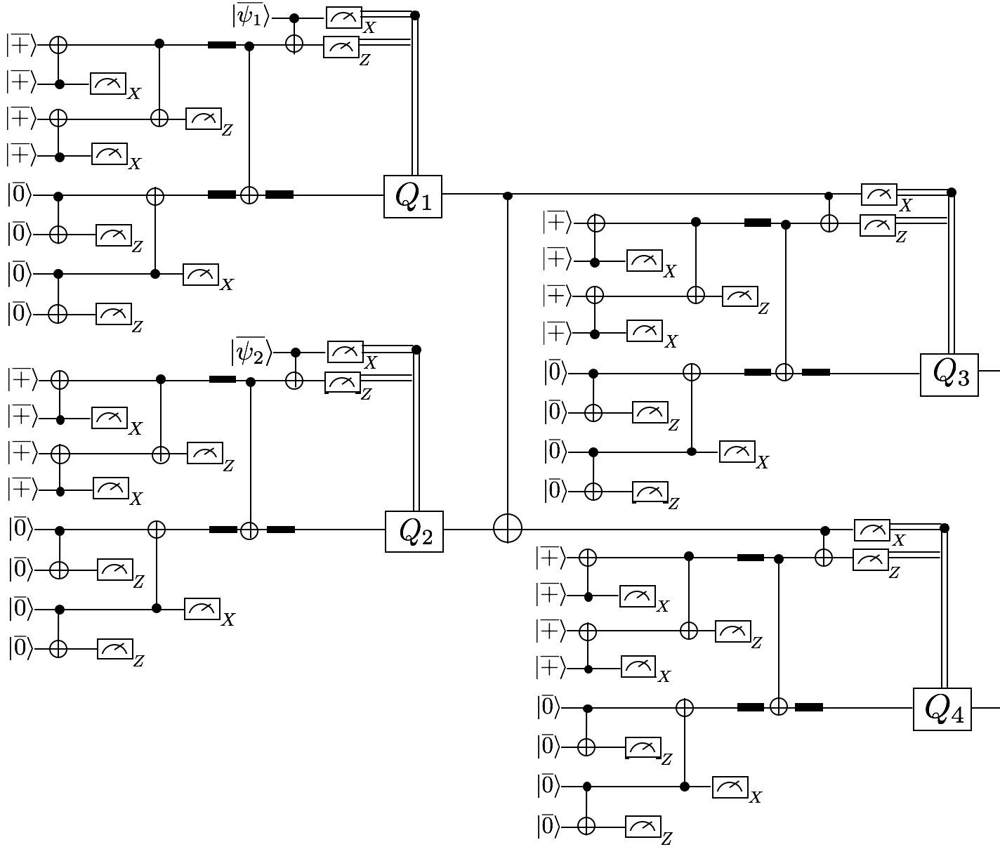
Figure 9: Full CNOT-exRec circuit using Knill error correction. Each Pauli operator $Q_{1},Q_{2},Q_{3}$ and $Q_{4}$ is used to correct errors in the initial data blocks as well as the complete teleportation protocol of the logical Bell measurement.

As in Steane-EC, the circuits for preparing the logical $|\overline{0}\rangle$ and $|\overline{+}\rangle$ states are not fault-tolerant and can result in high weight errors on the data. However, if the error correcting code is a CSS code, then we can use the same ancilla verification method presented in Section II.2 to make the full Knill-EC protocol fault-tolerant. In Fig. 9 we show the full CNOT-exRec circuit using Knill-EC. Note that for each EC unit, there is an extra idle qubit location compared to Steane-EC.

Lastly, we point out that another motivation for using Knill-EC is it’s ability to handle leakage errors. A leakage fault occurs when the state of a two-level system, which is part of a higher dimensional subspace, transitions outside of the subspace. In ATLeakage06 , it was shown how leakage faults can be reduced to a regular fault (which acts only on the qubit subspace) with the use of Leakage-Reduction Units (LRU’s). One of the most natural ways to implement LRU’s is through quantum teleportation MochonTeleportation04 . Since Knill-EC teleports the data block to the ancilla block, unlike in Steane-EC, LRU’s don’t need to be inserted on the input data block. However, LRU’s still need to be inserted after the preparation of every $|\overline{0}\rangle$ and $|\overline{+}\rangle$ states.

II.4 Naive decoder

Since the lookup table decoder scheme presented in previous sections is not scalable, it would be desirable to have a scalable and fast decoding scheme that can achieve competitive thresholds when paired with a deep neural decoder. In this section we provide a detailed description of a naive decoder which can replace the lookup table scheme in all of the above protocols.

We first note that the recovery operator $R_{s}$ for a measured syndrome $s$ can be written as Poulin06 ; DuclosRG1

$$R_{s}=\mathcal{L}(s)\mathcal{T}(s)\mathcal{G}(s)$$ (5)

which we will refer to as the LST decomposition of $E$. In Eq. 5, $\mathcal{L}(s)$ is a product of logical operators (operators in $N(\mathcal{S})\setminus\mathcal{S}$), $\mathcal{G}(s)$ is a product of stabilizers (operators in $\mathcal{S}$) and $\mathcal{T}(s)$ is a product of pure errors. Pure errors form an abelian group with the property that $T_{i}$ appears in $\mathcal{T}(s)$ if and only if the $i$’th syndrome bit is 1 (i.e. $[T_{i},T_{j}]=0$ and $[T_{j},g_{k}]=\delta_{j,k}$ where $g_{k}$ is the $k$’th stabilizer generator). Thus pure errors can be obtained from Gaussian elimination. Note that the choice of operators in $\mathcal{G}(s)$ will not effect the outcome of the recovered state. Consequently, given a measured syndrome $s$, decoding can be viewed as finding the most likely logical operator in $\mathcal{L}(s)$.

For a measured syndrome $s$, a naive decoding scheme is to always choose the recovery operator $R_{l}=\mathcal{T}(s)$ which is clearly suboptimal. However, for such a decoder, the decoding complexity results simply from performing the matrix multiplication $\mathbf{s}\ T$ where $\mathbf{s}=(s_{1},s_{2},\cdots,s_{n-k})$ is the syndrome written as a $1\times(n-k)$ vector and $T$ is a $(n-k)\times n$ matrix where the $j$’th row corresponds to $T_{j}$. The goal of all neural networks considered in Section III will then be to find the most likely operator $\mathcal{L}(s)$ from the input syndrome $l$.

The set of stabilizer generators, logical operators and pure errors for all the codes considered in this paper are provided in Table 8. Lastly, we point out that a version of the above decoding scheme was implemented in CrigerNN17 for the distance-three surface code.

II.5 Lookup table and naive decoder complexity

From a complexity theoretic point of view, read-out of an entry of an array or a hash table requires constant time. In hash tables, a hash function is calculated to find the address of the entry inquired. The hash function calculation takes the same processing steps for any entry, making this calculation $O(1)$. In the case of an array, the key point is that the array is a sequential block of the memory with a known initial pointer. Accessing any entry requires calculating its address in the memory by adding its index to the address of the beginning of the array. Therefore, calculating the address of an entry in an array also takes $O(1)$.

It remains to understand that accessing any location in the memory given its address is also $O(1)$ as far as the working of the memory hardware is concerned. This is the assumption behind random access memory (RAM) where accessing the memory comprises of a constant time operation performed by the multiplexing and demultiplexing circuitry of the RAM. This is in contrast with direct-access memories (e.g. hard disks, magnetic tapes, etc) in which the time required to read and write data depends on their physical locations on the device and the lag resulting from disk rotation and arm movement.

Given the explanation above, a decoder that relies solely on accessing recovery operators from an array operates in $O(1)$ time. This includes the lookup table and the inference mapping method of Section V.2 below.

For the naive decoder of Section II.4, we may also assume that the table of all pure errors (denoted as $T$ in Section II.4) is stored in a random access memory. However, the algorithm for generating a recovery from the naive decoder is more complicated than only accessing an element of $T$. With $n$ qubits and $n-k$ syndromes, for every occurrence of $1$ in the syndrome string, we access an element of $T$. The elements accessed in this procedure have to be added together. With parallelization, we may assume that a tree adder is used which, at every stage, adds two of the selected pure error strings to each other. Addition of every two pure error strings is performed modulo 2 which is simply the XOR of the two strings, which takes $O(1)$ time assuming parallel resources. The entire procedure therefore has a time complexity of $O((n-k)\log(n-k))$, again assuming parallel digital resources.

III Deep neural decoders

In most quantum devices, fully characterizing the noise model afflicting the system can be a significant challenge. Furthermore, for circuit level noise models which cannot be described by Pauli channels, efficient simulations of a codes performance in a fault-tolerant implementation cannot be performed without making certain approximations (a few exceptions for repetition codes can be found in YasunariEfficientRep17 ). However, large codes are often required to achieve low failure rates such that long quantum computations can be performed reliably. These considerations motivate fast decoding schemes which can adapt to unknown noise models encountered in experimental settings.

Recall from Section II.4 that decoding can be viewed as finding the most likely operator $L\in\mathcal{L}(\mathbf{s})$ given a measured syndrome $\mathbf{s}$. Since all codes considered in this paper encode a single logical qubit, the recovery operator for a measured syndrome $\mathbf{s}$ can be written as

$$R_{\mathbf{s}}=X_{L}^{b_{1}(\mathbf{s})}Z_{L}^{b_{2}(\mathbf{s})}\mathcal{T}(\mathbf{s})\mathcal{G}(\mathbf{s})$$ (6)

where $X_{L}$ and $Z_{L}$ are the codes logical $X$ and $Z$ operators and $b_{1}(\mathbf{s}),b_{2}(\mathbf{s})\in\mathbb{Z}_{2}$. In CWBL16 , a decoding algorithm applicable to general Markovian channels was presented for finding the coefficients $b_{1}(\mathbf{s})$ and $b_{2}(\mathbf{s})$ which optimized the performance of error correcting codes. However, the algorithm required knowledge of the noise channel and could not be directly applied to circuit level noise thus adding further motivation for a neural network decoding implementation.

In practice, the deep learning schemes described in this section can be trained as follows. First, to obtain the training set, the data qubits are fault-tolerantly prepared in a known logical $|\overline{0}\rangle$ or $|\overline{+}\rangle$ state followed by a round of fault-tolerant error correction (using either the lookup table or naive decoders). The encoded data is then measured in the logical $Z$ or $X$ basis yielding a -1 eigenvalue if a logical $X$ or $Z$ error occurred. The training set is constructed by repeating this sequence several times both for states prepared in $|\overline{0}\rangle$ or $|\overline{+}\rangle$. For each experiment, all syndromes are recorded as well as the outcome of the logical measurement. Given the most likely error $E$ with syndrome $s(E)=\mathbf{s}$ (in general $E$ will not be known), the neural network must then find the vector $\mathbb{b}=(b_{1}(\mathbf{s}),b_{2}(\mathbf{s}))$ such that $X_{L}^{b_{1}(\mathbf{s})}Z_{L}^{b_{2}(\mathbf{s})}R_{\mathbf{s}}E=I$ where $R_{\mathbf{s}}$ was the original recovery operator obtained from either the lookup table or naive decoders described in Section II.

Once the neural network is trained, to use it in the inference mode (as explained in Section V.2), a query to the network simply consists of taking as input all the measured syndromes and returning as output the vector $\mathbf{b}$. For Steane and Knill EC, the syndromes are simply the outcomes of the transversal $X$ and $Z$ measurements in the leading and trailing EC blocks. For the surface code, the syndromes are the outcomes of the ancilla measurements obtained from each EC round until the protocols presented in Section II.1 terminate.

Lastly, we note that a similar protocol was used in Baireuther2018machinelearning which also used the outcome of the final measurement on the data qubits to decode. However by using our method, once the neural network is trained, it only takes as input the measured syndromes in an EC round to compute the most likely $\mathbb{b}$.

III.1 Deep learning

Here we explain the generic framework of our deep learning experiments. We refer the reader to Goodfellow-et-al-2016 for an introduction to deep learning and to bishop2013pattern for machine learning methods in classification tasks.

Let $D\subseteq\mathcal{D}$ be a data set. In our case, $\mathcal{D}=S\times B$ is the set of all pairs of syndromes and error labels. Every element in $D$ and $\mathcal{D}$ is therefore a pair $(\mathbf{s},\mathbf{e})$ of measured syndromes $\mathbf{s}\in S$ and error labels $\mathbf{e}\in B$. The error labels can be different depending on how we model the learning problem. For instance, every $\mathbf{e}\in B$ can be a bit string carrying a prescription of recovery operators:

$$B=\{I,X,Y,Z\}^{\#\text{physical qubits}}.$$

There is however a major drawback in modelling the errors in the above fashion. For deep learning purposes the elements $\mathbf{e}\in B$ are represented in their 1-hot encoding, i.e. a bit string consisting of only a single 1, and zeros everywhere else. The 1-hot encoding therefore needs $|E|$ bits of memory allocated to itself which by the definitions above, grows exponentially in either the number of physical qubits.

Our solution for overcoming this exponentially growing model is to take advantage of the decomposition (Eq. 6) of the recovery operator and only predict vectors $\mathbf{b}=(b_{1}(\ell),b_{2}(\ell))$ as explained earlier. In other words, the elements of $B$ contain information about the logical errors remaining from the application of another auxiliary encoding scheme:

$$B=\{I,X,Y,Z\}^{\#\text{logical qubits}}.$$

The objective function

As customary in machine learning, the occurrences $x=(\mathbf{s},\mathbf{b})\in D$ are viewed as statistics gathered from a conditional probability distribution function $p(x)=\mathbb{P}(\mathbf{b}\,|\,\mathbf{s})$ defined over $S\times E$. The goal is then to approximate $p$ by another distribution $p_{w}$ which is easy to compute from a set of real-valued parameters $w$. The training phase in machine learning consists of optimizing the parameter vector $w$ such that $p_{w}$ is a good approximation of $p$. The optimization problem to solve is therefore

$$\min_{w}\quad \Delta(p,p_{w}).$$ (7)

Here $\Delta$ is some notion of distance in the space of probability distribution functions which, when applied to machine learning, is also called the loss function. In our case, the distance is the softmax cross entropy as explained here. The softmax function with respect to $p$ is given via

$$\rho(x)=\frac{e^{p(x)}}{\sum_{x\in\mathcal{D}}e^{p(x)}}.$$ (8)

From this definition it is obvious that no normalization of the dataset $D$ is needed since softmax already results in a probability distribution function. The cross entropy function

$$H(\pi_{1},\pi_{2})=H(\pi_{1})+D_{KL}(\pi_{1}|\!|\pi_{2})=-\sum_{x}\pi_{1}(x)\log\pi_{2}(x)$$ (9)

is then applied after softmax. This turns (7) into

$$\min_{w}\quad h(w)=H(\rho(p),\rho(p_{w})).$$ (10)

Optimization of the softmax cross-entropy is a common practice in classification problems.

The neural network

A neural network is a directed graph equipped with a random variable assigned to each of its nodes. The elements of the parameter vector $w$ are assigned either to an edge of the graph or a node of the graph (in the former case they are called weights and in the latter case they are called biases). The roll of the neural network in solving (10) is to facilitate a gradient descent direction for the vector $w$ in (10). This is achieved by imposing the random variables of each node to be a function of the random variables with incoming edges to the former one. The common choice for such a functional relationship is an affine transformation composed with a nonlinear function (called the activation function) with an easy to compute derivative. Given every node $v$ of the neural network, we define:

$$X_{v}=a_{v}\left(\sum_{u\rightarrow v}w_{uv}X_{u}+w_{v}\right).$$ (11)

The simplest activation function is of course the identity. Historically, the sigmoid function $\sigma(x)=\frac{1}{1+e^{-x}}$ was the most commonly used activation function and is motivated by its appearance in training restricted Boltzmann machines. By performing a change of variables, one obtains the trigonometric activation function $\tanh(x)$. These activation functions can cause the learning rate to slow down due to vanishing gradients in the early layers of deep neural networks, and this is the motivation for other proposed activation functions such as the rectified linear unit $\operatorname{relu}(x)$. Design and analysis of activation functions is an important step in machine learning LeCun1998 ; Nair:2010:RLU:3104322.3104425 ; pmlr-v9-glorot10a .

The first and last layers of the network are known as the visible layers and respectively correspond to the input and output data (in our case the tuples $(\mathbf{s},\mathbf{b})\in S\times B$ as explained above). Successive applications of Eq. 11 restricts the conditional distribution $p_{w}(\mathbf{b}\,|\,\mathbf{s})$ into a highly nonlinear function $f(w,\mathbf{s},\mathbf{b})$, for which the derivatives with respect to the parameters $w$ are easy to compute via the chain rule. We may therefore devise a gradient descent method for solving Eq. 10 by successive choices of descent directions starting from the deep layers and iterating towards the input nodes. In machine learning, this process is known as back-propagation.

Remark.

The softmax function (Eq. 8) is in other words the activation function between the last two layers of the neural network.

Layouts

Although deep learning restricts the approximation of $p_{w}(\mathbf{b}|\mathbf{s})$ to functions of the form $f(w,\mathbf{s},\mathbf{b})$ as explained above, the latter has tremendous representation power, specially given the freedom in choice of the layout of the neural network. Designing efficient layouts for various applications is an artful and challenging area of research in machine learning. In this paper, we discuss three such layouts and justify their usage for the purposes of our deep neural decoding.

Feedforward neural network. By this we mean a multi-layer neural network consisting of consecutive layers, each layer fully connected to the next one. Therefore, the underlying undirected subgraph of the neural network consisting of the neurons of two consecutive layers is a complete bipartite graph. In the case that the neural network only consists of the input and output layers (with no hidden layers), the network is a generalization of logistic regression (known as the softmax regression method).

Recurrent neural network (RNN). RNNs have performed incredibly well in speech recognition and natural language processing tasks Fernandez:2007:ARN:1778066.1778092 ; Sutskever:2014:SSL:2969033.2969173 ; 45446 ; 2015arXiv151200103G . The network is designed to resemble a temporal sequence of input data, with each input layer connecting to the rest of the network at a corresponding temporal epoch. The hidden cell of the network could be as simple as a single feedforward layer or more complicated. Much of the success of RNNs is based on peculiar designs of the hidden cell such as the Long-Short Term Memory (LSTM) unit as proposed in Hochreiter:1997:LSM:1246443.1246450 .

Convolutional neural network (CNN). CNNs have been successfully used in image processing tasks Schmidhuber:2012:MDN:2354409.2354694 ; ILSVRC15 . The network is designed to take advantage of local properties of an image by probing a kernel across the input image and calculating the cross-correlation of the kernel vector with the image. By applying multiple kernels, a layer of features is constructed. The features can then be post-processed via downsizing (called max-pooling) or by yet other feedforward neural networks.

In sections III.2 and III.3, we present further details about applications of these neural networks to the error-decoding task.

Stochastic gradient descent

Since the cross-entropy in Eq. 9 is calculated by a weighted sum over all events $x\in\mathcal{D}$, it is impractical to exactly calculate it or its derivatives as needed for backpropagation. Instead, one may choose only a single sample $x=(\mathbf{s},\mathbf{b})$ as a representative of the entire $\mathcal{D}$ in every iteration. Of course, this is a poor approximation of the true gradient but one hopes that the occurrences of the samples according to the true distribution would allow for the descent method to ‘average out’ over many iterations. This method is known as stochastic gradient descent (SGD) or online learning. We refer the reader to Nemirovski:2009:RSA:1654243.1654247 and NIPS2003_2365 and the references therein for proofs of convergences and convergence rates of online learning. In practice, a middle ground between passing through the entire dataset and sampling a single example is observed to perform better for machine learning tasks LeCun1998 : we fix a batch size and in every iteration average over a batch of the samples of this size. We call this approach batch gradient descent (also called mini-batch gradient descent for better contrast). The result is an update rule for the parameter vector of the form $w_{t+1}\leftarrow w_{t}+\Delta_{t}$ where $\Delta_{t}$ is calculated as

$$\Delta_{t}=-\eta_{t}\nabla_{t-1},$$

for some step size $\eta_{t}$, where $\nabla_{t-1}=\nabla_{w_{t-1}}\tilde{h}(w_{t-1})$ to simplify the notation. Here $\tilde{h}$ is an approximation of $h$ in (10) by the partial sum over the training batch. Finding a good schedule for $\eta_{t}$ can be a challenging engineering task that will be addressed in Section III.1.5. Depending on the optimization landscape, SGD might require extremely large numbers of iterations for convergence. One way to improve the convergence rate of SGD is to add a momentum term Rumelhart:1986:LIR:104279.104293 :

$$\Delta_{t}=p\Delta_{t-1}-\eta_{t}\nabla_{t-1}.$$

On the other hand, it is convenient to have the schedule of $\eta_{t}$ be determined through the training by a heuristic algorithm that adapts to the frequency of every event. The method AdaGrad was developed to allow much larger updates for infrequent samples Pennington14glove:global :

$$\Delta_{t}=-\operatorname{diag}\left({\frac{\eta}{\sqrt{\Sigma_{ti}+\varepsilon}}}\right)\nabla_{t-1}.$$

Here $\Sigma_{ti}$ is the sum of the squares of all previous values of the $i$-th entry of the gradient. The quantity $\varepsilon$ is a small (e.g. $10^{-8}$) smoothening factor in order to avoid dividing by zero. The denominator in this formula is called the root mean squared (RMS). An important advantage of AdaGrad is the fact that the freedom in the choice of the step-size schedule is restricted to choosing one parameter $\eta$, which is called the learning rate.

Finally RMSProp is an improvement on AdaGrad in order to slow down the aggressive vanishing rate of the gradients in AdaGrad tielemanH12 . This is achieved by adding a momentum term to the root mean squared:

$$\operatorname{diag}(\Sigma_{t})=p\operatorname{diag}(\Sigma_{t-1})+(1-p)\nabla_{t-1}\nabla_{t-1}^{T}.$$

Hyperparameter tuning

From the above exposition, it is apparent that a machine learning framework involves many algorithms and design choices. The performance of the framework depends on optimal and consistent choices of the free parameters of each piece, the hyperparameters. For example, while a learning rate of $10^{-3}$ might be customary for a small dataset such as that of MNIST digit recognition, it might be a good choice for a small feedforward network and a bad choice for the RNN used in our problem scenario. In our case, the hyperparameters include the decay rate, the learning rate, the momentum in RMSProp, the number of hidden nodes in each layer of the network, the number of hidden layers and filters, and some categorical variables such as the activation function of each layer, the choice of having peepholes or not in the RNN.

It would be desirable if a metaheuristic can find appropriate choices of hyperparameters. The challenges are

1. Costly function evaluation: the only way to know if a set of hyperparameters is appropriate for the deep learning framework, is to run the deep learning algorithm with these parameters;

2. Lack of a gradient-based solution: the solution of the deep learning framework does not have a known functional dependence on the hyperparameters. Therefore, the metaheuristic has no knowledge of a steepest descent direction.

It is therefore required for the metaheuristic to be (1) sample efficient and (2) gradient-free. Having a good metaheuristic as such is extremely desirable, since:

1. The performance of the ML framework might be more sensitive to some parameters than to others. It is desirable for the metaheuristic to identify this.

2. Compatibility of the parameters: leaving the hypertuning job to a researcher can lead to search in very specific regimes of hyperparameters that are expected to be good choices individually but not in combination.

3. Objectivity of the result: a researcher might spend more time tuning the parameters of their proposal than on a competing algorithm. If the same metaheuristic is used to tune various networks, such as feedforward networks, RNNs and CNNs, the result would be a reliable comparison between all suggestions.

Bayesian optimization. Bayesian optimization mockus1989bayesian ; mockus1989bayesian is a nonlinear optimization algorithm that associates a surrogate model to its objective function and modifies it at every function evaluation. It then uses this surrogate model to decide which point to explore next for a better objective value JMLR:v15:martinezcantin14a . Bayesian optimization is a good candidate for hypertuning as it is sample efficient and can perform well for multi-modal functions without a closed formula. A disadvantage of Bayesian optimization to keep in mind is that it relies on design choices and parameters of its own that can affect its performance in a hyperparameter search.

III.2 Steane and Knill EC deep neural decoder for the CNOT-exRec

The simplest deep neural decoder for any dataset is a feedforward network with none or many hidden layers, each layer fully connected to the next one. The input layer receives the bit strings of $X$ and $Z$ syndromes. And the output layer corresponds to the $X$ and $Z$ recovery operators on the physical qubits of the code. Since multiple physical qubits might be used to encode a single logical operator, a better choice is for the output layer to encode whether an auxiliary (but efficient) decoding scheme is causing logical faults or not. The goal would be to predict such logical faults by the deep neural decoder and when the deep neural decoder predicts such a fault, we will impose a logical Pauli operator after the recovery suggested by the auxiliary decoder. The 1-hot encoding in two bits, $10$ and $01$, respectively stand for $I$ and $X$ for the $X$-errors, and it stands for $I$ and $Z$ for the $Z$ errors.

From our early experiments it became apparent that it is beneficial to half separate $X$ and $Z$ neural networks that share a loss function, that is the sum of the soft-max cross entropies of the two networks. Fig. 10 shows the schematics of such a feedforward network.

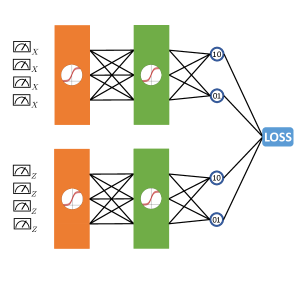
Figure 10: Schematics of a feedforward network consisting of disjoint $X$ and $Z$ networks. There may be none, one or multiple hidden layers with different activation functions. The output layers correspond to logical $I$- and $X$-errors for the $X$ network and to logical $I$- and $Z$-errors for the $Z$ network. The activation function of the last layer before the error layer is the identity since in the softmax cross entropy loss function, the activation (by softmax) is already included.

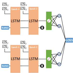
Figure 11: Schematics of a network consisting of two disjoint $X$ and $Z$ RNNs. Each RNN receives the syndromes of leading and trailing EC rounds as inputs for two epochs of its LSTM unit. The internal state of the first copy is initialized randomly and the internal state of the last copy is garbage-collected. The hidden state of the last copy of the LSTM unit is then fully connected to a hidden layer with user-defined activation function. This hidden unit is then fully connected to output nodes denoted by $01$ and $10$ which are respectively the one-hot encoding of the prediction as to whether an $X$-recovery or a $Z$-recovery operation is needed on the output qubits from exRec-CNOT. The loss function is the sum of the loss functions of the two networks.

The CNOT-exRec RNN

In the case of the CNOT-exRec, the leading EC rounds have temporal precedence to the trailing EC rounds. Therefore a plausible design choice for the deep neural decoder would be to employ an RNN with two iterations on the hidden cell. In the first iteration, the syndrome data from the leading EC rounds are provided and in the second iteration the syndrome data from the trailing EC rounds are provided. A demonstration of this network is given in Fig. 11.

Figure 12: Schematics of a long-short term memory (LSTM) cell. Without the red circuits, this neural network is called a simple LSTM unit. The red circuit is called peepholes. An LSTM cell with peepholes can outperform a simple LSTM cell in some tasks. There are four hidden layers with user-defined activation functions in an LSTM unit known as the forget layer (F), input layer (I), hidden layer (H) and the output layer (O). There are four 2 to 1 logical gates in the unit that depending on the sign written on them applies an element-wise operation between the vectors fed into the logical gates. There is also a 1 to 1 logical gate that applies an element-wise $tanh$ function on its input vector. The internal state of an LSTM unit serves as the backbone of a sequence of replications of the LSTM unit. The roll of the internal state is to capture temporal features of the sequence of input data.

The hidden cell of the RNN may be an LSTM, or an LSTM with peepholes as shown in Fig. 12. An LSTM cell consists of an internal state which is a vector in charge of carrying temporal information through the unrolling of the LSTM cell in time epochs. There are 4 hidden layers. The layer $H$ is the ‘actual’ hidden layer including the input data of the current epoch with the previous hidden layer from the previous epoch. The activation of $H$ is usually $\tanh$. The ‘input’ layer $I$ is responsible for learning to be a bottleneck on how important the new input is, and the ‘forget’ layer $F$ is responsible for creating a bottleneck on how much to forget about the previous epochs. Finally the ‘output’ layer $O$ is responsible for creating a bottleneck on how much data is passed through from the new internal state to the new hidden layer. The peepholes in Fig. 12 allow the internal state to also contribute in the hidden layers $F$, $I$ and $O$.

III.3 Surface code deep neural decoder

Other than the multi-layer feedforward network of Fig. 10, there are two other reasonable designs for a deep neural network when applied to the surface code.

The surface code RNN

In the fault-tolerant scheme of the rotated surface code, multiple rounds of error correction are done in a sequence as explained in Sec. II.1. It is therefore encouraging to consider an RNN with inputs as syndromes of the consecutive EC rounds. The network looks similar to that of Fig. 11 except that the number of epochs is equal to the maximum number of EC rounds. In particular, the fault tolerant scheme for the distance-three rotated surface code consists of three EC rounds. In the case of the distance-five surface code, the maximum number of EC rounds through the algorithm of Sec. II.1 is six. If the rounds of EC stop earlier, then the temporal input sequence of syndrome strings is padded by repeating the last syndrome string. As an example, if after three rounds the fault tolerant scheme terminates, then the input syndromes of epochs three to six of the RNN are all identical and equal to the third syndrome string.

The surface code CNN

The errors, syndromes and recovery operators of the surface code are locally affected by each other. It is therefore suggestive to treat the syndromes of the surface code as a 2-dimensional array, the same way pixels of an image are treated in image processing tasks. The multiple rounds of EC would account for a sequence of such images, an animation. Therefore a 3-dimensional CNN appears to be appropriate. This means that the kernels of the convolutions are also 3-dimensional, probing the animation along the two axes of each image and also along the third axis representative of time.

Through our test-driven design, it became obvious that treating the $X$ and $Z$ syndromes as channels of the same 3-dimensional input animation is not a good choice. Instead, the $X$ and $Z$ syndromes should be treated as disjoint inputs of disjoint networks which in the end contribute to the same loss function. Notice that in the case of the distance-five rotated surface code, the $X$ network receives a 3D input of dimensions $3\times 4\times 6$ and the $Z$ network receives a 3D input of dimensions $4\times 3\times 6$. To create edge features, the inputs were padded outwards symmetrically, i.e. with the same binary values as their adjacent bits. This changes the input dimensions to $4\times 5\times 6$ and $5\times 4\times 6$ respectively for the $X$ and $Z$ animations. Via similar experiments, we realized that two convolutional layers do a better job in capturing patterns in the syndromes data. The first convolutional layer is probed by a $3\times 3\times 3$ kernel, and the second layer is probed by a $4\times 4\times 4$ kernel. After convolutional layers, a fully connected feedforward layer with dropouts and relu activations is applied to the extracted features and then the softmax cross-entropy is measured. The schematic of such a neural network is depicted in Fig. 13.

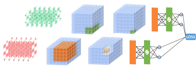
Figure 13: Schematics of a deep neural decoder for the distance-five rotated surface code. The network consists of two disjoint neural networks contributing to the same loss function via softmax cross entropy. Each neural network consists of two layers of 3D CNNs. The first layer consists of a number of filters, each filter performing a convolution of a $3\times 3\times 3$ kernel by the input syndromes. The second 3D CNN layer uses $4\times 4\times 4$ kernels. The colored boxes demonstrate how each layer is padded in order for the size of the 3D layers to be preserved. When the kernel dimension is even for instance, the padding from the top and left are of size 1, and the padding from the bottom and right are of size 2.

IV Numerical experiments

In the experimental results reported in this section, multiple data sets were generated by various choices of physical error rates ranging between $p=1.0\times 10^{-4}$ to $p=2.0\times 10^{-3}$. Every data set consisted of simulating the circuit-level depolarizing channel (see Section II for a detailed description of the noise model) for the corresponding circuit, and included the syndrome and resulting error bit strings in the data set. Note that the error strings are only used as part of the simulation to compute the vector $\mathbb{b}$ of logical faults. In an actual experiment, $\mathbb{b}$ would be given directly (see the discussion above Section III.1). We excluded the cases were both the syndrome and error strings were all zeros. The simulation was continued until a target number of non-zero training samples were gathered. The target size of the training data set was chosen as $2\times 10^{6}$ for distance-three codes, and as $2\times 10^{7}$ for distance-five codes.

Hypertuning was performed with the help of BayesOpt JMLR:v15:martinezcantin14a . In every hypertuning experiment, each query consisted of a full round of training the deep learning network on 90% of the entire dataset and cross-validating on the remaining 10%. It is important to add randomness to the selection of the training and cross-validating data sets so that the hyperparameters do not get tuned for a fixed choice of data entries. To this aim, we uniformly randomly choose an initial element in the entire data set, take the 90% of the dataset starting from that initial element (in a cyclic fashion) as the training set, and the following 10% as the test dataset.

The cross-entropy of the test set is returned as the final outcome of one query made by the hypertuning engine. For all hypertuning experiments, 10 initial queries were performed via Latin hypercube sampling. After the initial queries, 50 iterations of hypertuning were performed.

For each fault-tolerant error correction scheme, hypertuning was performed on only a single data set (i.e. only for one of the physical error rates). A more meticulous investigation may consist of hypertuning for each individual physical error rate separately but we avoided that, since we empirically observed that the results are independent of the choice of hypertuning data set. At any rate, the data chosen for distance-three codes was the one corresponding to $p=4\times 10^{-4}$. For the distance-five rotated surface code, $p=6.0\times 10^{-4}$ and for the 19-qubit color code using Steane and Knill-EC, $p=1.0\times 10^{-3}$ were chosen for hypertuning.

Hyperparameters chosen from this step were used identically for training all other data sets. For every data set (i.e. every choice of physical fault rate $p$) the deep learning experiment was run 10 times and in the diagrams reported below the average and standard deviations are reported as points and error bars. In every one of the 10 runs, the training was done on 90% of a data set, and cross validation was done on the remaining 10%. All the machine learning experiments were implemented in Python 2.7 using TensorFlow 1.4tensorflow2015-whitepaper on top of CUDA 9.0 running installed on TitanXp and TitanV GPUs produced by NVIDIANickolls:2008:SPP:1365490.1365500 .

All experiments are reported in Fig. 19–Fig. 25. Before continuing with detailed information on each experiment, we refer the reader to Table 1 where we provide the largest ratios of the pseudo-thresholds obtained using a neural network decoder to pseudo-thresholds obtained from bare lookup table decoders of each fault-tolerant protocol considered in this paper.

FTEC	Lookup	DND	Ratio
$d=3$ Steane	$p_{\text{th}}=2.10\times 10^{-4}$	$p_{\text{th}}=3.98\times 10^{-4}$	1.90
$d=5$ Steane	$p_{\text{th}}=1.43\times 10^{-3}$	$p_{\text{th}}=2.17\times 10^{-3}$	1.52
$d=3$ Knill	$p_{\text{th}}=1.76\times 10^{-4}$	$p_{\text{th}}=2.22\times 10^{-4}$	1.26
$d=5$ Knill	$p_{\text{th}}=1.34\times 10^{-3}$	$p_{\text{th}}=1.54\times 10^{-3}$	1.15
$d=3$ Surface code	$p_{\text{th}}=2.57\times 10^{-4}$	$p_{\text{th}}=3.18\times 10^{-4}$	1.24
$d=5$ Surface code	$p_{\text{th}}=5.82\times 10^{-4}$	$p_{\text{th}}=7.11\times 10^{-4}$	1.22

Table 1: Pseudo-thresholds for the 6 fault-tolerant error correction protocols considered in the experiments. The second column corresponds to the highest pseudo-thresholds obtained from a bare lookup table decoder whereas the third column gives the highest pseudo-thresholds using neural network decoders. The last column corresponds to the ratio between the pseudo-thresholds obtained from the best neural network decoders and the lookup table decoders.

Steane-EC CNOT-exRec for the $[\![7,1,3]\!]$ code

parameter	lower bound	upper bound
decay rate	$0.0$	$1.0-10^{-6.0}$
momentum	$0.0$	$1.0-10^{-6.0}$
learning rate	$10^{-5.0}$	$10^{-1.0}$
initial std	$10^{-3.0}$	$10^{-1.0}$
num hiddens	$100$	$1000$

Table 2: Bayesian optimization parameters for the CNOT-exRec of the $[\![7,1,3]\!]$ code using Steane and Knill-EC and the distance-three rotated surface code. Here the decay rate, momentum and learning rate pertain to the parameters of RMSProp. The row ‘initial std’ refers to the standard deviation of the initial weights in the neural networks, the mean of the weights was set to zero. The initial biases of the neural networks were set to zero. The row ‘num hiddens’ refers to the number of hidden nodes in the layers of neural network. This parameter is optimized for each layer of the neural network independently (e.g. for a feedforward network consisting of 3 hidden layers, there are 3 numbers of hidden nodes to be tuned). For an RNN this number indicates the number of hidden nodes in every one of the 4 hidden layers of the LSTM unit (all of the same size).

The considered continuous and integer hyperparameters are given in Table 2.

We also tuned over the categorical parameters of Table 3.

parameter	values
activation functions	relu, tanh, sigmoid, identity
numbers of hidden layers	0, 1, 2, …

Table 3: Categorical hyperparameters. Optimizations over activation functions was only performed for the distance-three Steane code. Since rectified linear units showed better results, we committed to this choice for all other error correction schemes. However, for the second categorical hyperparameter (the numbers of hidden layers), the search was performed for all error correction schemes separately and was stopped at the numbers of hidden layers where the improvements in the results discontinued.

The categorical parameters are tuned via grid-search. We observed that for all choices of neural networks (feedforward networks with various numbers of hidden layers and recurrent neural networks with or without peepholes), the rectified linear unit in the hidden layers and identity for the last layer resulted in the best performance. We accepted this choice of activation functions in all other experiments without repeating a grid-search.

Figs. 19 and 19 compare the performance of the feedforward and RNN decoders that respectively use the lookup table and naive-decoder as their underlying decoders, respectively referred to as LU-based deep neural decoders (LU-DND) and PE-based deep neural decoders (PE-DND). We use PE since naive-decoders correct by applying pure errors. We observe that softmax regression (i.e. zero hidden layers) is enough to get results on par with the lookup table method in the LU-based training method, this was not the case in the PE-based method. The RNNs perform well but they are outperformed by two-hidden-layer feedforward networks. Additional hidden layers improve the results in deep learning. However, since this is in expense for a cross-entropy optimization in higher dimensions, the training of deeper networks is significantly more challenging. This trade-off is the reason the feedforward networks improve up to two hidden layers, but passing to three and higher numbers of hidden layers gave worse results (not reported in these diagrams).

We finally observe that PE-DND with even a single hidden layer feedforward network is almost on par with the LU-DND with two hidden layers. This is an impressive result given the fact that a table of pure errors grows linearly in the number of syndromes, but a lookup table grows exponentially. We believe this is a result of the fact that logical faults are much more likely to occur when using recovery operators which only consist of products of pure-errors, the training sets are less sparse and therefore deep learning is able to capture more patterns for the classification task at hand.

Knill-EC CNOT-exRec for the $[\![7,1,3]\!]$ code

The hypertuning of continuous variables was done using the same bounds as in Table 2. Figs. 19 and 19 respectively show the results of LU-DND and PE-DND methods. The best results were obtained by feedforward networks with respectively 3 and 2 hidden layers, in both cases slightly outperforming RNNs.

Distance-three rotated surface code

Similar to the previous distance-three codes, we compared using RNNs with feedforward networks with multiple hidden layers. We observed that the feedfoward network with a single hidden layer achieves the best performance and RNNs do not improve the results. Also consistent with the distance-three CNOT- exRec results, the PE-based DND can perform as good as the LU-based one (and slightly improves upon it). Results of these experiments are reported in Figs. 19 and 19.

Steane-EC CNOT-exRec for the $[\![19,1,5]\!]$ code

As the size of the input and output layers of DNNs grow, the ranges of the optimal hyperparameters change. For the distance-five Steane exRec circuit applied to the $[\![19,1,5]\!]$ color code, the considered hyperparameter ranges (allowing smaller orders of magnitudes for the initial weight standard deviations and much smaller learning rates) are given in Table 4.

parameter	lower bound	upper bound
decay rate	$0.0$	$1.0-10^{-6.0}$
momentum	$0.0$	$1.0-10^{-6.0}$
learning rate	$10^{-7.0}$	$10^{-3.0}$
initial std	$10^{-5.0}$	$10^{-3.0}$
num hiddens	$100$	$1000$

Table 4: Bayesian optimization parameters for $d=5$ Steane and Knill CNOT-exRecs. Given the larger size of the training sets and longer input strings, for these datasets, smaller orders of magnitudes for the initial weight standard deviations and much smaller learning rates were explored.

Figs. 25 and 25 show that the PE-DNDs has a slightly harder time with pattern recognition compared to the LU-DNDs. Nevertheless, both methods significantly improve the pseudo-thresholds of the distance-five Steane-EC scheme, with no advantage obtained from using an RNN over a 2-hidden layer feedforward network. In both experiments, the 3-hidden layer feedforward networks also did not result any improvements.

Knill-EC CNOT-exRec for the $[\![19,1,5]\!]$ code

The hyperparameter ranges used for hypertuning were similar to those obtained for the Steane-EC CNOT-exRec applied to the $[\![19,1,5]\!]$ code. Given the effectiveness of the 2-hidden layer feedforward network, this feedforward neural network was chosen for the Knill exRec $d=5$ experiment. We see a similar improvement on the pseudo-threshold of the error correction scheme using either of LU-DND and PE-DND.

Distance-five rotated surface code

For rotated surface codes, we only considered numerical simulations using one EC rather than the full exRec. This choice was made to be consistent with previous analyses of the surface codes performance.

The hyperparameter ranges used for hypertuning the feedforward neural networks were chosen according to Table 5.

parameter	lower bound	upper bound
decay rate	$0.0$	$1.0-10^{-6.0}$
momentum	$0.0$	$1.0-10^{-6.0}$
learning rate	$10^{-6.0}$	$10^{-2.0}$
initial std	$10^{-6.0}$	$10^{-2.0}$
num hiddens	$100$	$1000$

Table 5: Bayesian optimization parameters for the distance-five rotated surface code. The parameter search is in a slightly tighter domain than in the case of the distance-five Knill and Steane CNOT-exRecs in view of the empirical initial tests performed.

As explained in the previous section, a CNN engineered appropriately could be a viable layout design for large surface codes. Beside previous hyperparameters, we now also need to tune the number of filters, and drop-out rate. A summary of the settings for Bayesian optimization are given in Table 6.

parameter	lower bound	upper bound
decay rate	$0.0$	$1.0-10^{-6.0}$
momentum	$0.0$	$1.0-10^{-6.0}$
learning rate	$10^{-6.0}$	$10^{-2.0}$
initial std	$10^{-6.0}$	$10^{-2.0}$
num hiddens	$100$	$1000$
keep rate	$0.0$	$1.0$
num filters	$5$	$10$

Table 6: Bayesian optimization parameters for a 3-dimensional CNN. The filters were fixed to be $3\times 3\times 3$ and $4\times 4\times 4$ but their quantities were tuned. Since CNNs are larger and deeper than other networks considered in this paper, they are more prone to vanishing gradients. Therefore it is beneficial to consider drop-outs in the hidden layer after feature extraction. The hyperparameter corresponding to drop-outs is ‘keep rate’ allowing more drop-outs when it is smaller.

We compare the PE-based and LU-based feedforward networks with the CNN proposed in Section III.3. Figs. 25 and 25 show that feedforward networks with 2 hidden layers result in significant improvements both using the PE-based and LU-based DNDs. The 3D-CNN is slightly improving the results of the feedforward network in PE-DND but is only slightly better than the lookup table based method in the LU-DND case. The best overall performance is obtained by using a feedfoward network with 2 hidden layers for the LU-DND. A slightly less performant result can also be obtained if the PE-DND method is used in conjunction with either of the 2-hidden layer feedforward network or the 3D convolutional neural network.

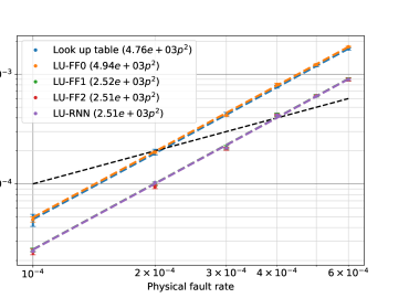
Figure 14: LU-DND for the distance-three Steane CNOT-exRec.

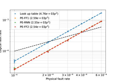
Figure 15: PE-DND for the distance-three Steane CNOT-exRec.

Figure 16: LU-DND for the distance-three Knill CNOT-exRec.

Figure 17: PE-DND for the distance-three Knill CNOT-exRec.

Figure 18: LU-DND for the distance-three surface code.

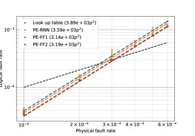
Figure 19: PE-DND for the distance-five surface code.

In Fig. 19–Fig. 19 each data point has the height on the vertical axis being the average of 10 logical fault rates collected for each physical fault rate $p$ specified on the horizontal axis. Error bars represent the standard deviation from these average values. For each DND-based decoder, the cuve-fitting method used is a non-linear least square fitting between the average logical fault rates as a function of the physical fault rates, and a quadratic monomial.

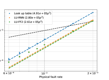
Figure 20: LU-DND for the distance-five Steane CNOT-exRec.

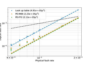
Figure 21: PE-DND for the distance-five Steane CNOT-exRec.

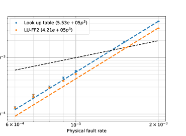
Figure 22: LU-DND for the distance-five Knill CNOT-exRec.

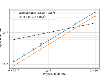
Figure 23: PE-DND for the distance-five Knill CNOT-exRec.

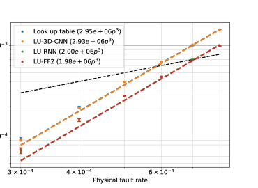
Figure 24: LU-DND for the distance-five surface code.

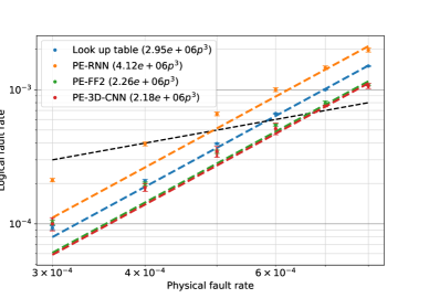
Figure 25: PE-DND for the distance-five surface code.

In Fig. 25–Fig. 25 data points, averages and error bars are obtaines in a similar fashion to Fig. 19–Fig. 19. The cuve-fitting method is also a non-linear least square method, this time fitting a cubic monomial through the data points.

V Performance analysis

In this section we consider the efficiency of the deep neural decoders in comparison to the lookup table decoders described in Sections II.1 and II.2. The size of a lookup table grows exponentially in the number of syndromes therefore making lookup table based decoding intractable as the codes grow. However, it is important to note that as long as the size of the lookup table allows for storage of the entire table in memory, as described in Section II.5, the lookup from an array or a hash table happens effectively in $O(1)$ time. Therefore a lookup table based decoding scheme would be the most efficient decoder by far. A similar approach to a lookup table decoder is possible by making an inference mapping from all the possible input strings of a trained neural decoder. This method is discussed in Section V.1. For larger codes, neither a lookup table decoder, nor an inference mapping decoder is an option due to exponentially growing memory usage.

More complicated decoders such as minimum weight perfect matching can be extremely inefficient solutions for decoding despite polynomial asymptotic complexity. With gates operating at 100Mhz (that is $10$ns gate times) 0034-4885-80-10-106001 , which is much faster than the state of the art, the simplest quantum algorithms foreseen to run on near term devices would require days of runtime on the system 2017PNAS..114.7555R . With the above gate times, the CNOT-exRec using Steane and Knill EC units as well as the multiple rounds of EC for surface codes would take as small as a hundred nanoseconds. In order to perform active error correction, we require classical decoding times to be implemented on (at worst) a comparable time scale as the EC units, and therefore merely a complexity theoretic analysis of a decoding algorithm is not enough for making it a viable solution. Alternatively, given a trained DND, inference of new recovery operations from it is a simple algorithm requiring a sequence of highly parallelizable matrix multiplications. We will discuss this approach in Section V.2 and Section V.3.

V.1 Inference mapping from a neural decoder

For codes of arbitrary size, the most time-performant way to use a deep neural decoder is to create an array of all inputs and outputs of the DNN in the test mode (i.e. an inference map which stores all possible syndromes obtained from an EC unit and assigns each combination to a recovery operator). This is possible for distance-three fault-tolerant EC schemes such as Steane, Knill and surface codes (as well as other topological schemes such as those used for color codes). For all these codes, the memory required to store the inference map is 2.10 megabytes. This method is not feasible for larger distance codes. For the Knill and Steane-EC schemes applied to the $[\![19,1,5]\!]$ color code, the memory required is 590 exabytes and for the distance-five rotated surface code it is $2.79\times 10^{24}$ exabytes.

V.2 Fast inference from a trained neural network

An advantage of a deep neural decoder is that the complications of decoding are to be dealt with in the training mode of the neural network. The trained network is then used to suggest recovery operations. The usage of the neural network in this passive step, i.e. without further training, is called the inference mode. Once the neural network is trained, usage of it in the inference mode requires only a sequence of few simple arithmetic operations between the assigned valued of its input nodes and the trained weights. This makes inference an extremely simple algorithm and therefore a great candidate for usage as a decoder while the quantum algorithm is proceeding.

However, even for an algorithm as simple as inference, further hardware and software optimization is required. For example, CrigerNN17 predicts that on an FPGA (field-programmable gate array) every inference from a single layer feedforward network would take as long as 800ns. This is with the optimistic assumption that float-point arithmetic (in 32 and 64-bit precision) takes 2.5 to 5 nanoseconds and only considering a single layer feedforward network.

In this section, we consider alternative optimization techniques for fast inference. We will consider a feedforward network with two hidden layers given their promising performance in our experiments.

Network quantization

Fortunately, quantum error correction is not the only place where fast inference is critical. Search engines, voice and speech recognition, image recognition, image tagging, and many more applications of machine learning are nowadays critical functions of smart phones and many other digital devices. As the usage grows, the need for efficient inference from the trained models of these applications grow. It is also convenient to move such inference procedures to the usage platforms (e.g. the users smart phones and other digital devices) than merely a cloud based inference via a data centre. Recent efforts in high performance computing has focused on fabricating ASICs (Application Specific Integrated Circuits) specifically for inference from neural networks. Google’s TPU (Tensor Processing Unit) 2017arXiv170404760J is being used for inference in Google Search, Google Photos and in DeepMind’s AlphaGo against one of the the world’s top Go player, Lee Sedol.

It is claimed that the reduction in precision of a trained neural network from 32-bit float point precision in weights, biases, and arithmetic operations, to only 8-bit fixed point preserves the quality of inference from trained models 37631 . This procedure is called network quantization. There is no mathematical reason to believe that the inference quality should hold up under network quantization. However, the intuitive explanation has been that although the training mode is very sensitive to small variations of parameters and hyperparameters, and fluctuations of the high precision weights of the network in individual iterations of training is very small, the resulting trained network is in principle robust to noise in data and weights.

The challenge in our case is that in quantum error correction, the input data is already at the lowest possible precision (each neuron attains 0 or 1, therefore only using a single bit). Furthermore, an error in the input neurons results in moving from one input syndrome to a completely different one (for instance, as opposed to moving from a high resolution picture to a low resolution, or poorly communicated one in an image processing task). We therefore see the need to experimentally verify whether network quantization is a viable approach to high-performance inference from a DND.

Fig. 26 demonstrates an experiment to validate network quantization on a trained DND. Using 32-bit float-point precision, the results of Fig. 19 show that the trained DND improves the logical fault rate from $1.95\times 10^{-4}$ obtained by lookup table methods to $9.45\times 10^{-5}$ obtained by the LU-DND with 2 hidden layers. We observe that this improvement is preserved by the quantized networks with 8 bits and even 7 bits of precision using fix-point arithmetic.

We now explain how the quantized network for this experiment was constructed. Let us assume the available precision is up to $k$ bits. First, the weights and biases of the network are rescaled and rounded to nearest integers such that the resulting parameters are all integers between $-2^{k-1}+1$ and $2^{k-1}$ stored as signed $k$-bit integers. Each individual input neuron only requires a single bit since they store zeros and ones. But we also require that the result of feedforward obtained by multiplications and additions and stored in the hidden layers is also a $k$-bit signed integer. Unlike float-point arithmetic, fixed point arithmetic operations can and often overflow. The result of multiplication of two $k$-bit fixed-point integers can span $2k$ bits in the worst case. Therefore the results of each hidden layer has to be shifted to a number of significant digits and the rightmost insignificant digits have to be forgotten. For instance, in the case of the CNOT-exRec with Steane EC units, each input layer has 12 bits, which get multiplied by 12 signed integers each with $k$-bit fixed point precision. A bias with $k$-bit fixed point precision is then added to the result. We therefore need at most $k+\lceil\log_{2}(13)\rceil$-bits to store the result. Therefore the rightmost $\lceil\log_{2}(13)\rceil$ bits have to be forgotten. If the weights of the trained neural network are symmetric around zero, it is likely that only a shift to the right by $2$ bits is needed in this case. Similarly, if each hidden layer has $L$ nodes, the largest shift needed would be $\lceil\log_{2}(L+1)\rceil$ but most likely $\lceil\log_{2}(L+1)\rceil-1$ shifts suffices. In the experiment of Fig. 26, each hidden layer had 1000 nodes and the feedforward results were truncated in their rightmost 9 digits.

Figure 26: Quantization of the feedforward neural network with 2 hidden layers, trained on the Steane EC dataset at a physical error rate of $p=2\times 10^{-4}$. Each point is calculated as the average logical error rate obtained from 10 rounds of training and cross-validating similar to the experiments in Section IV.

V.3 Classical arithmetic performance

In the previous section we showed that 8-bit fixed point arithmetic is all that is needed for high quality inference from the trained deep neural decoder. We now consider a customized digital circuit for the inference task and estimate how fast the arithmetic processing units of this circuit have to be in order for the inference to be of practical use for active quantum error correction.

The runtime of a digital circuit is estimated by considering the time that is required for the electric signal to travel through the critical path of the logical circuit Rabaey:2008:DIC:1817056 , the path with the longest sequence of serial digital operations.

Fig. 27 shows the critical path of a circuit customized to carry inference in a feedforward network with 2 hidden layers. Since the input neurons represent syndrome bits, multiplying them with the first set of weights can be done with parallel AND between the syndrome bit and the weight bits. The rectified linear unit is efficient since it only requires a NAND between the sign of the 8-bit signed integer with the other 7 bits of it. The most expensive units in this circuit are the $8\times 8$ multipliers and adders. Every $8\times 8$ multiplier gives a 16-bit fixed point integer which is then shifted 8-bits to the right by ignoring the first 8-bits. The total time delay $t_{\mathrm{TOT}}$ of this path in the circuit is

$$t_{\mathrm{TOT}}=t_{\mathrm{AND}}+\lceil\log(S+1)\rceil\ t_{\mathrm{ADD}}+t_{\mathrm{MAX}}\\ +\sum_{i=1}^{H}(t_{\mathrm{NOT}}+t_{\mathrm{AND}}+t_{\mathrm{MULT}}+\lceil\log(L_{i}+1)\rceil\ t_{\mathrm{ADD}})$$ (12)

where $H$ is the number of hidden layers and $L_{i}$ is the number of neurons in the $i$-th hidden layer. From a complexity theoretic point of view this is promising since it shows that the cost of inference is logarithmic in the number of syndromes and the size of hidden layers, and linear in the number of hidden layers. For a feedforward network with two hidden layers and at most $1000$ neurons in each hidden layer,

$$t_{\mathrm{TOT}}=3\ t_{\mathrm{AND}}+2\ t_{\mathrm{NOT}}+2\ t_{\mathrm{MULT}}+t_{\mathrm{MAX}}\\ +\left(\lceil\log(S+1)\rceil+20\right)\ t_{\mathrm{ADD}}.$$ (13)

Since the adders contribute the most in the above time delay, let us give an upper bound on how fast the adder units need to be in order for the total time delay to be comparable to the runtime of the fault-tolerant quantum error correction protocols considered in this paper.

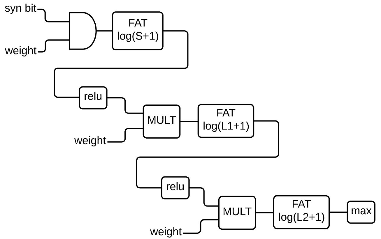
Figure 27: The critical path of a custom inference circuit. Every syndrome bit represents an input node of the neural network and is multiplied by 8-bit integer weights. A set of such products are added together and together with an 8-bit bias integer to find the activation on a node of the first hidden layer. Given $S$ input syndromes, this amounts to the addition of $S+1$ integers which can be done with a tree of 8-bit integer full-adders (Full-Adder Tree or FAT for short) of depth $\log(S+1)$. After the quantized rectified linear unit, a similar procedure is iterated for the first hidden layer with the full-adder tree of depth $\log(L_{1}+1)$ where $L_{1}$ is the number of neurons in the first hidden layer. This pattern continues for other hidden layers. The MAX unit compares two 8-bit integers and outputs 0 if the first one is bigger and 1 if the second one is bigger.

In Table 7 we compute upper bounds on the adder units for the fault-tolerant error correction protocols considered in this paper. We emphasize that this estimation is by the optimistic assumption that all independent arithmetic operations are done in parallel. In reality, this is not possible due to limitations in area and power consumption of the ASIC. Also considering that multiple rounds of inference have to happen, a pipeline architecture should be considered for independent batches of inference on the ASIC. Lastly, the time for multiplier unit and the comparator are ignored since (if all independent jobs are done in parallel) there are only two serial multipliers in the critical path. With all of these considerations, the last row of this table should be interpreted as an optimistic allowed time for the adder units and that the actual adder delays should be well below these numbers.

FTEC	FTEC	Syn	Num	Adder
Circuit	Depth	Size	Adders	Leniency
$d=3$ Steane	6	12	24	2.5ns
$d=5$ Steane	6	36	26	2.3ns
$d=3$ Knill	8	12	24	3.3ns
$d=5$ Knill	8	36	26	3.1ns
$d=3$ Surface code	18	12	24	7.5ns
$d=5$ Surface code	36	72	27	13.3ns

Table 7: FTEC depth is the depth of the FTEC circuit. For Steane and Knill EC, this is the depth of the CNOT-exRec circuit (excluding the ancilla verification steps) and in the surface code, it is the depth of the circuit for multiple rounds of syndrome measurement (note that for the distance 5 surface code we considered the worst case of 6 syndrome measurement rounds). The syndrome size is only that of one of $X$ and $Z$ since the inference for $X$ and $Z$ logical errors can happen in parallel and independently. The adder time leniency is calculated based on 10ns quantum gate delays. Therefore, it is the depth of the FTEC multiplied by 10ns and divided by the number of adders.

In particular we conclude that in order to perform active error correction with the methods summarized in Table 7 on a quantum computer with $10$ns gate delays, the classical control unit of the quantum computer has to comprise of arithmetic units that are fast enough to perform arithmetic operations well below the time limits reported in the last column of this table. In hardware engineering, there are many approaches to implementation of arithmetic and logical units Parhami:1999:CAA:318930 . Without going into the details of the circuit designs we mention that the adder leniencies in Table 7 are in reach of high performance VLSI 25695 ; 488718 , but could be challenging to achieve using FPGAs Wolf:2004:FSD:983326 ; Xing ; 831434 .

V.4 Limitations of deep neural decoders

We interpret the results of this section to suggest that, once implemented on a high performance computing platform, inference can be computed efficiently from a trained deep neural decoder. Further, the results of Section IV show that with a large enough training set, neural network decoders achieve lower logical failure rates compared to the lookup table schemes presented in this paper. However, this does not imply that deep neural decoders are scalable. As the size of the codes grow, training the neural decoders becomes much more daunting. This is due to the fact that deep learning classifiers are not viable solutions for sparse classification problems. As the codes become better and/or physical error rates become smaller, the training samples become more and more sparse, providing less and less effective training samples for the neural network. Without nontrivial training samples, the neural networks learn “zeros” rather than capturing significant patterns in the data set.

As evidence for the effect of sparsity of the dataset on successful training of the deep neural decoding we refer the reader to an experiment reported in Fig. 28. In this experiment, the DND is trained on the dataset corresponding to the highest physical fault rate $p=2\times 10^{-3}$. The same trained DND is used to cross-validate on test datasets for all other physical fault rates. We observe that this DND is more successful in recovery inference for smaller physical error rates, even though it is trained on a “wrong” dataset. It is important to note that this experiment does not provide an improved method for training a neural network for error correction on a physical realization of a quantum processor. Firstly, in any manufactured quantum device the error model will not be entirely known (and is not necessarily close to a theoretic noise model such as the depolarizing channel). And secondly, the error of the device cannot be intensified intentionally for the purpose of training a deep neural decoder, to be later used on a less noisy device.

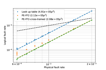
Figure 28: A comparison between two training procedures for the CNOT-exRec of the $[\![19,1,5]\!]$ color code using Steane-EC units. The orange dots are the results of training a feedforward network with 2 hidden layers as reported also in Fig. 25. In this case, the DND is trained on a given physical error rate $p$ and tested on a test dataset for the same physical error rate. We observe that the logical error rate does not exactly follow a cubic growth since the training is less successful when the physical error rate is small. The green line, demonstrates the performance of the same DND if trained only for the largest physical error rate $p=2\times 10^{-3}$, and later on tested on test datasets from every other physical error rate. The neural network captured syndrome and recovery patterns occurring in the CNOT-exRec that are valid for all values of physical error rate. As previously explained, such a training scenario is not possible for real-world experiments, or on physical realizations of quantum computers.

VI Conclusion

To conclude, the main contributions of this paper were considering multiple fault-tolerant schemes and using several neural network architectures to train decoders in a full circuit-level noise framework. Although our analysis was done for Pauli channels, we expect that for non-Pauli noise models, the improvements could be even more significant than what was observed in our work. Evidence of this can be found in CWBL16 where decoders were adapted to non-Pauli noise channels.

From a machine learning point of view, we applied state-of-the-art techniques used in training neural networks. While considering many network designs, we used the same hyperparameter tuning methodology to achieve unbiased and reliable results. Consequently, we successfully observed a clear advantage in using deep networks in comparison with single hidden layer networks and regression methods. On the other hand, we provided clear evidence of the realistic limitations of deep learning in low noise rate regimes. In particular, scaling the neural network to large distance codes appears to be a significant challenge. For large scale quantum computations, decoders that work less well than neural decoders trained on small distance codes but which are scalable would clearly be the better option. Lastly, we gave a rigorous account of the digital hardware resources needed for inference and runtime analysis of the critical path of the customized digital circuitry for high performance inference.

There remains many interesting future directions for designing improved and efficient decoders which work well in fault-tolerant regimes. One such avenue would be to tailor machine learning algorithms specifically designed for decoding tasks. In particular, finding machine learning algorithms which work well with sparse data would be of critical importance. It would also be interesting to apply the methods introduced in this work to actual quantum devices that are currently being developed. It most certainly will be the case that fault-tolerant designs will be tailored to a particular quantum architecture. This would lead to further areas in which machine learning could be extremely useful for finding improved decoders.

VII Acknowledgements

Both authors contributed equally to this work. We acknowledge Steve G. Weiss for providing the necessary computing resources. The authors would also like to thank Ben Criger, Raymond Laflamme, Thomas O’Brien, Xiaotong Ni, Barbara Terhal, Giacomo Torlai, Tomas Jochym-O’Connor, Aleksander Kubica and Ehsan Zahedinejad for useful discussions. C.C. acknowledges the support of NSERC through the PGS D scholarship. P.R. acknowledges the support of the government of Ontario and Innovation, Science and Economic Development Canada.

$[\![7,1,3]\!]$ Steane code	$[\![9,1,3]\!]$ (Surface-17) code	$[\![19,1,5]\!]$ color code	$[\![25,1,5]\!]$ (Surface-49) code
$g^{(x)}_{1}=X_{4}X_{5}X_{6}X_{7}$	$g^{(x)}_{1}=X_{1}X_{2}X_{4}X_{5}$	$g^{(x)}_{1}=X_{1}X_{2}X_{3}X_{4}$	$g^{(x)}_{1}=X_{1}X_{2}X_{6}X_{7}$
$g^{(x)}_{2}=X_{2}X_{3}X_{6}X_{7}$	$g^{(x)}_{2}=X_{7}X_{8}$	$g^{(x)}_{2}=X_{1}X_{3}X_{5}X_{7}$	$g^{(x)}_{2}=X_{11}X_{12}X_{16}X_{17}$
$g^{(x)}_{3}=X_{1}X_{3}X_{5}X_{7}$	$g^{(x)}_{3}=X_{2}X_{3}$	$g^{(x)}_{3}=X_{5}X_{7}X_{8}X_{11}X_{12}X_{13}$	$g^{(x)}_{3}=X_{21}X_{22}$
$g^{(z)}_{1}=Z_{4}Z_{5}Z_{6}Z_{7}$	$g^{(x)}_{4}=X_{5}X_{6}X_{8}X_{9}$	$g^{(x)}_{4}=X_{1}X_{2}X_{5}X_{6}X_{8}X_{9}$	$g^{(x)}_{4}=X_{2}X_{3}$
$g^{(z)}_{2}=Z_{2}Z_{3}Z_{6}Z_{7}$	$g^{(z)}_{1}=Z_{1}Z_{4}$	$g^{(x)}_{5}=X_{6}X_{9}X_{16}X_{19}$	$g^{(x)}_{5}=X_{7}X_{8}X_{12}X_{13}$
$g^{(z)}_{3}=Z_{1}Z_{3}Z_{5}Z_{7}$	$g^{(z)}_{2}=Z_{2}Z_{3}Z_{5}Z_{6}$	$g^{(x)}_{6}=X_{16}X_{17}X_{18}X_{19}$	$g^{(x)}_{6}=X_{17}X_{18}X_{22}X_{23}$
	$g^{(z)}_{3}=Z_{4}Z_{5}Z_{7}Z_{8}$	$g^{(x)}_{7}=X_{8}X_{9}X_{10}X_{11}X_{16}X_{17}$	$g^{(x)}_{7}=X_{3}X_{4}X_{8}X_{9}$
	$g^{(z)}_{4}=Z_{6}Z_{9}$	$g^{(x)}_{8}=X_{10}X_{11}X_{12}X_{15}$	$g^{(x)}_{8}=X_{13}X_{14}X_{18}X_{19}$
		$g^{(x)}_{9}=X_{12}X_{13}X_{14}X_{15}$	$g^{(x)}_{9}=X_{23}X_{24}$
		$g^{(z)}_{1}=Z_{1}Z_{2}Z_{3}Z_{4}$	$g^{(x)}_{10}=X_{4}X_{5}$
		$g^{(z)}_{2}=Z_{1}Z_{3}Z_{5}Z_{7}$	$g^{(x)}_{11}=X_{9}X_{10}X_{14}X_{15}$
		$g^{(z)}_{3}=Z_{5}Z_{7}Z_{8}Z_{11}Z_{12}Z_{13}$	$g^{(x)}_{12}=X_{19}X_{20}X_{24}X_{25}$
		$g^{(z)}_{4}=Z_{1}Z_{2}Z_{5}Z_{6}Z_{8}Z_{9}$	$g^{(z)}_{1}=Z_{1}Z_{6}$
		$g^{(z)}_{5}=Z_{6}Z_{9}Z_{16}Z_{19}$	$g^{(z)}_{2}=Z_{2}Z_{3}Z_{7}Z_{8}$
		$g^{(z)}_{6}=Z_{16}Z_{17}Z_{18}Z_{19}$	$g^{(z)}_{3}=Z_{4}Z_{5}Z_{9}Z_{10}$
		$g^{(z)}_{7}=Z_{8}Z_{9}Z_{10}Z_{11}Z_{16}Z_{17}$	$g^{(z)}_{4}=Z_{6}Z_{7}Z_{11}Z_{12}$
		$g^{(z)}_{8}=Z_{10}Z_{11}Z_{12}Z_{15}$	$g^{(z)}_{5}=Z_{8}Z_{9}Z_{13}Z_{14}$
		$g^{(z)}_{9}=Z_{12}Z_{13}Z_{14}Z_{15}$	$g^{(z)}_{6}=Z_{10}Z_{15}$
			$g^{(z)}_{7}=Z_{11}Z_{16}$
			$g^{(z)}_{8}=Z_{12}Z_{13}Z_{17}Z_{18}$
			$g^{(z)}_{9}=Z_{14}Z_{15}Z_{19}Z_{20}$
			$g^{(z)}_{10}=Z_{16}Z_{17}Z_{21}Z_{22}$
			$g^{(z)}_{11}=Z_{18}Z_{19}Z_{23}Z_{24}$
			$g^{(z)}_{12}=Z_{20}Z_{25}$
$T^{(x)}_{1}=X_{4}$	$T^{(x)}_{1}=X_{1}$	$T^{(x)}_{1}=X_{4}$	$T^{(x)}_{1}=X_{1}$
$T^{(x)}_{2}=X_{2}$	$T^{(x)}_{2}=X_{3}$	$T^{(x)}_{2}=X_{3}X_{4}$	$T^{(x)}_{2}=X_{3}$
$T^{(x)}_{3}=X_{1}$	$T^{(x)}_{3}=X_{8}$	$T^{(x)}_{3}=X_{13}X_{14}$	$T^{(x)}_{3}=X_{5}$
$T^{(z)}_{1}=Z_{3}Z_{7}$	$T^{(x)}_{4}=X_{9}$	$T^{(x)}_{4}=X_{5}X_{7}$	$T^{(x)}_{4}=X_{3}X_{7}$
$T^{(z)}_{2}=Z_{5}Z_{7}$	$T^{(z)}_{1}=Z_{4}$	$T^{(x)}_{5}=X_{18}X_{19}$	$T^{(x)}_{5}=X_{5}X_{9}$
$T^{(z)}_{3}=Z_{6}Z_{7}$	$T^{(z)}_{2}=Z_{7}$	$T^{(x)}_{6}=X_{6}X_{9}X_{17}$	$T^{(x)}_{6}=X_{5}X_{10}$
	$T^{(z)}_{3}=Z_{2}Z_{4}$	$T^{(x)}_{7}=X_{6}X_{9}$	$T^{(x)}_{7}=X_{3}X_{7}X_{11}$
	$T^{(z)}_{4}=Z_{6}$	$T^{(x)}_{8}=X_{6}X_{9}X_{10}$	$T^{(x)}_{8}=X_{18}X_{24}$
		$T^{(x)}_{9}=X_{6}X_{9}X_{10}X_{15}$	$T^{(x)}_{9}=X_{5}X_{10}X_{15}$
		$T^{(z)}_{1}=Z_{2}Z_{5}Z_{7}$	$T^{(x)}_{10}=X_{17}X_{18}X_{24}$
		$T^{(z)}_{2}=Z_{1}Z_{2}$	$T^{(x)}_{11}=X_{24}$
		$T^{(z)}_{3}=Z_{13}Z_{14}$	$T^{(x)}_{12}=X_{5}X_{10}X_{15}X_{20}$
		$T^{(z)}_{4}=Z_{5}Z_{7}$	$T^{(z)}_{1}=Z_{6}$
		$T^{(z)}_{5}=Z_{18}Z_{19}$	$T^{(z)}_{2}=Z_{16}$
		$T^{(z)}_{6}=Z_{6}Z_{9}Z_{16}Z_{18}Z_{19}$	$T^{(z)}_{3}=Z_{21}$
		$T^{(z)}_{7}=Z_{6}Z_{9}$	$T^{(z)}_{4}=Z_{2}Z_{6}$
		$T^{(z)}_{8}=Z_{5}Z_{7}Z_{8}Z_{11}$	$T^{(z)}_{5}=Z_{12}Z_{16}$
		$T^{(x)}_{9}=Z_{6}Z_{9}Z_{11}Z_{12}$	$T^{(z)}_{6}=Z_{21}Z_{22}$
			$T^{(z)}_{7}=Z_{8}Z_{12}Z_{16}$
			$T^{(z)}_{8}=Z_{19}Z_{25}$
			$T^{(z)}_{9}=Z_{21}Z_{22}Z_{23}$
			$T^{(z)}_{10}=Z_{4}Z_{8}Z_{12}Z_{16}$
			$T^{(z)}_{11}=Z_{14}Z_{19}Z_{25}$
			$T^{(z)}_{12}=Z_{25}$
$X_{L}=X^{\otimes 7}$,$Z_{L}=Z^{\otimes 7}$	$X_{L}=X_{3}X_{5}X_{7}$,$Z_{L}=Z_{1}Z_{5}Z_{9}$	$X_{L}=X^{\otimes 19}$,$Z_{L}=Z^{\otimes 19}$	$X_{L}=X_{5}X_{9}X_{13}X_{17}X_{21}$,$Z_{L}=Z_{1}Z_{7}Z_{13}Z_{19}Z_{25}$

Table 8: Table containing a list of the stabilizer generators (second row), pure errors (third row) and logical operators (fourth row) for all the codes considered in this article.

References

- (1) “Intel Press Kit.” https://newsroom.intel.com/press-kits/quantum-computing/. Accessed: 2018-02-16.
- (2) “IBM Q Experience.” https://quantumexperience.ng.bluemix.net/qx/devices. Accessed: 2018-02-16.
- (3) “Riggeti QPU.” http://pyquil.readthedocs.io/en/latest/qpu_overview.html. Accessed: 2018-02-16.
- (4) C. Neill, P. Roushan, K. Kechedzhi, S. Boixo, S. V. Isakov, V. Smelyanskiy, R. Barends, B. Burkett, Y. Chen, Z. Chen, B. Chiaro, A. Dunsworth, A. Fowler, B. Foxen, R. Graff, E. Jeffrey, J. Kelly, E. Lucero, A. Megrant, J. Mutus, M. Neeley, C. Quintana, D. Sank, A. Vainsencher, J. Wenner, T. C. White, H. Neven, and J. M. Martinis, “A blueprint for demonstrating quantum supremacy with superconducting qubits,” ArXiv e-prints, Sept. 2017.
- (5) C. Vuillot, “Is error detection helpful on ibm 5q chips ?,” arXiv:quant-ph/1705.08957, 2017.
- (6) A. R. Calderbank and P. W. Shor, “Good quantum error-correcting codes exist,” Phys. Rev. A, vol. 54, pp. 1098–1105, 1996.
- (7) A. W. Steane, “Enlagement of calderbank-shor-steane quantum codes,” IEEE. Trans.Inform. Theory, vol. 45, no. 7, pp. 2492–2495, 1999.
- (8) E. Knill, “Fault-tolerant postselected quantum computation: schemes,” arXiv:quant-ph/0402171, 2004.
- (9) E. Knill, “Quantum computing with realistically noisy devices,” Nature, vol. 434, no. 7029, pp. 39–44, 2005.
- (10) A. G. Fowler, M. Mariantoni, J. M. Martinis, and A. N. Cleland, “Surface codes: Towards practical large-scale quantum computation,” Phys. Rev. A, vol. 86, p. 032324, 2012.
- (11) R. Chao and B. W. Reichardt, “Quantum error correction with only two extra qubits,” arXiv:quant-ph/1705.02329, 2017.
- (12) R. Chao and B. W. Reichardt, “Fault-tolerant quantum computation with few qubits,” arXiv:quant-ph/1705.05365, 2017.
- (13) C. Chamberland and M. E. Beverland, “Flag fault-tolerant error correction with arbitrary distance codes,” Quantum, vol. 2, p. 53, Feb. 2018.
- (14) E. Knill, R. Laflamme, and W. H. Zurek, “Threshold accuracy for quantum computation,” arXiv: quant-ph/9610011, 1996.
- (15) T. Jochym-O’Connor and R. Laflamme, “Using concatenated quantum codes for universal fault-tolerant quantum gates,” Phys. Rev. Lett., vol. 112, p. 010505, 2014.
- (16) A. Paetznick and B. W. Reichardt, “Universal fault-tolerant quantum computation with only transversal gates and error correction,” Phys. Rev. Lett., vol. 111, p. 090505, 2013.
- (17) J. T. Anderson, G. Duclos-Cianci, and D. Poulin, “Fault-tolerant conversion between the steane and reed-muller quantum codes,” Phys. Rev. Lett., vol. 113, p. 080501, 2014.
- (18) H. Bombín, “Dimensional jump in quantum error correction,” arXiv:1412.5079, 2014.
- (19) T. J. Yoder, R. Takagi, and I. L. Chuang, “Universal fault-tolerant gates on concatenated stabilizer codes,” Phys. Rev. X, vol. 6, p. 031039, Sep 2016.
- (20) T. J. Yoder and I. H. Kim, “The surface code with a twist,” Quantum, vol. 1, p. 2, Apr. 2017.
- (21) C. Chamberland, J. J. Wallman, S. Beale, and R. Laflamme, “Hard decoding algorithm for optimizing thresholds under general markovian noise,” Phys. Rev. A, vol. 95, p. 042332, 2017.
- (22) A. S. Darmawan and D. Poulin, “Tensor-network simulations of the surface code under realistic noise,” Phys. Rev. Lett., vol. 119, p. 040502, Jul 2017.
- (23) A. S. Darmawan and D. Poulin, “An efficient general decoding algorithm for the surface code,” arXiv:1801.01879, 2018.
- (24) J. Edmonds, “Paths, trees, and flowers,” Canadian Journal of mathematics, vol. 17, no. 3, pp. 449–467, 1965.
- (25) A. G. Fowler, A. C. Whiteside, A. L. McInnes, and A. Rabbani, “Topological code autotune,” Phys. Rev. X, vol. 2, p. 041003, Oct 2012.
- (26) D. Poulin, “Optimal and efficient decoding of concatenated quantum block codes,” Phys. Rev. A., vol. 74, p. 052333, 2006.
- (27) G. Torlai and R. G. Melko, “Neural decoder for topological codes,” Phys. Rev. Lett., vol. 119, p. 030501, Jul 2017.
- (28) S. Varsamopoulos, B. Criger, and K. Bertels, “Decoding small surface codes with feedforward neural networks,” Quantum Science and Technology, vol. 3, no. 1, p. 015004, 2018.
- (29) P. Baireuther, T. E. O’Brien, B. Tarasinski, and C. W. J. Beenakker, “Machine-learning-assisted correction of correlated qubit errors in a topological code,” Quantum, vol. 2, p. 48, Jan. 2018.
- (30) N. P. Breuckmann and X. Ni, “Scalable neural network decoders for higher dimensional quantum codes,” arXiv:quant-ph/1710.09489, 2017.
- (31) N. Maskara, A. Kubica, and T. Jochym-O’Connor, “Advantages of versatile neural-network decoding for topological codes,” arXiv:1802.08680, 2018.
- (32) P. Aliferis, D. Gottesman, and J. Preskill, “Quantum accuracy threshold for concatenated distance–3 codes,” Quant. Inf. Comput., vol. 6, pp. 97–165, 2006.
- (33) D. Gottesman, Stabilizer Codes and Quantum Error Correction. PhD thesis, California Institute of Technology, 1997.
- (34) D. Gottesman, “An introduction to quantum error correction and fault-tolerant quantum computation,” Proceedings of Symposia in Applied Mathematics, vol. 68, pp. 13–58, 2010.
- (35) P. Aliferis, D. Gottesman, and J. Preskill, “Accuracy threshold for postselected quantum computation,” Quant. Inf. Comput., vol. 8, pp. 181–244, 2008.
- (36) D. Gottesman, “The heisenberg representation of quantum computers, talk at,” in International Conference on Group Theoretic Methods in Physics, Citeseer, 1998.
- (37) S. Bravyi and A. Kitaev, “Quantum codes on a lattice with boundary,” arXiv:quant-ph/9811052, 1998.
- (38) E. Dennis, A. Kitaev, A. Landhal, and J. Preskill, “Topological quantum memory,” Journal of Mathematical Physics, vol. 43, pp. 4452–4505, 2002.
- (39) A. Kitaev, “Fault-tolerant quantum computation by anyons,” Annals of Physics, vol. 303, no. 1, pp. 2 – 30, 2003.
- (40) Y. Tomita and K. M. Svore, “Low-distance surface codes under realistic quantum noise,” Phys. Rev. A., vol. 90, p. 062320, 2014.
- (41) X.-G. Wen, “Quantum orders in an exact soluble model,” Phys. Rev. Lett., vol. 90, p. 016803, Jan 2003.
- (42) A. G. Fowler, “Minimum weight perfect matching of fault-tolerant topological quantum error correction in average o(1) parallel time,” Quantum Info. Comput., vol. 15, pp. 145–158, Jan. 2015.
- (43) A. G. Fowler, A. C. Whiteside, and L. C. L. Hollenberg, “Towards practical classical processing for the surface code: Timing analysis,” Phys. Rev. A, vol. 86, p. 042313, Oct 2012.
- (44) G. Duclos-Cianci and D. Poulin, “Fast decoders for topological quantum codes,” Phys. Rev. Lett., vol. 104, p. 050504, Feb 2010.
- (45) G. Duclos-Cianci and D. Poulin, “Fault-tolerant renormalization group decoder for abelian topological codes,” Quant. Inf. Comput., vol. 14, no. 9 & 10, pp. 0721–0740), 2014.
- (46) S. Bravyi and J. Haah, “Quantum self-correction in the 3d cubic code model,” Phys. Rev. Lett., vol. 111, p. 200501, Nov 2013.
- (47) J. R. Wootton and D. Loss, “High threshold error correction for the surface code,” Phys. Rev. Lett., vol. 109, p. 160503, Oct 2012.
- (48) N. Delfosse and N. H. Nickerson, “Almost-linear time decoding algorithm for topological codes,” arXiv:quant-ph/1709.06218, 2017.
- (49) J. Conrad, C. Chamberland, N. P. Breuckmann, and B. M. Terhal, “The small stellated dodecahedron code and friends,” arXiv:quant-ph/1712.07666, 2017.
- (50) A. W. Steane, “Active stabilization, quantum computation, and quantum state synthesis,” Phys. Rev. Lett., vol. 78, no. 11, p. 2252, 1997.
- (51) B. M. Terhal, “Quantum error correction for quantum memories,” Reviews of Modern Physics, vol. 87, p. 307, 2015.
- (52) C. Chamberland, P. Iyer, and D. Poulin, “Fault-tolerant quantum computing in the Pauli or Clifford frame with slow error diagnostics,” Quantum, vol. 2, p. 43, Jan. 2018.
- (53) D. P. DiVincenzo and P. Aliferis, “Effective fault-tolerant quantum computation with slow measurements,” Phys. Rev. Lett., vol. 98, p. 020501, 2007.
- (54) A. Paetznick and B. W. Reichardt, “Fault-tolerant ancilla preparation and noise threshold lower bounds for the 23-qubit golay code,” Quant. Inf. Compt., vol. 12, pp. 1034–1080, 2011.
- (55) C. Chamberland, T. Jochym-O’Connor, and R. Laflamme, “Thresholds for universal concatenated quantum codes,” Phys. Rev. Lett., vol. 117, p. 010501, 2016.
- (56) C. Chamberland, T. Jochym-O’Connor, and R. Laflamme, “Overhead analysis of universal concatenated quantum codes,” Phys. Rev. A, vol. 95, p. 022313, 2017.
- (57) H. Bombin and M. A. Martin-Delgado, “Topological quantum distillation,” Phys. Rev. Lett., vol. 97, p. 180501, Oct 2006.
- (58) P. O. Boykin, T. Mor, M. Pulver, V. Roychowdhury, and F. Vatan, “On universal and fault-tolerant quantum computing: A novel basis and a new constructive proof of universality for shor’s basis,” in Foundations of Computer Science, 1999. 40th Annual Symposium on, pp. 486–494, IEEE, 1999.
- (59) P. Aliferis and B. M. Terhal, “Fault-tolerant quantum computation for local leakage faults,” Quant. Inf. Comput., vol. 7, pp. 139–156, 2007.
- (60) C. Mochon, “Anyon computers with smaller groups,” Phys. Rev. A, vol. 69, p. 032306, Mar 2004.
- (61) Y. Suzuki, K. Fujii, and M. Koashi, “Efficient simulation of quantum error correction under coherent error based on the nonunitary free-fermionic formalism,” Phys. Rev. Lett., vol. 119, p. 190503, Nov 2017.
- (62) I. Goodfellow, Y. Bengio, and A. Courville, Deep Learning. MIT Press, 2016. http://www.deeplearningbook.org.
- (63) C. Bishop, Pattern Recognition and Machine Learning. Information science and statistics, Springer, 2013.
- (64) Y. LeCun, L. Bottou, G. B. Orr, and K. R. Müller, Efficient BackProp, pp. 9–50. Berlin, Heidelberg: Springer Berlin Heidelberg, 1998.
- (65) V. Nair and G. E. Hinton, “Rectified linear units improve restricted boltzmann machines,” in Proceedings of the 27th International Conference on International Conference on Machine Learning, ICML’10, (USA), pp. 807–814, Omnipress, 2010.
- (66) X. Glorot and Y. Bengio, “Understanding the difficulty of training deep feedforward neural networks,” in Proceedings of the Thirteenth International Conference on Artificial Intelligence and Statistics (Y. W. Teh and M. Titterington, eds.), vol. 9 of Proceedings of Machine Learning Research, (Chia Laguna Resort, Sardinia, Italy), pp. 249–256, PMLR, 13–15 May 2010.
- (67) S. Fernández, A. Graves, and J. Schmidhuber, “An application of recurrent neural networks to discriminative keyword spotting,” in Proceedings of the 17th International Conference on Artificial Neural Networks, ICANN’07, (Berlin, Heidelberg), pp. 220–229, Springer-Verlag, 2007.
- (68) I. Sutskever, O. Vinyals, and Q. V. Le, “Sequence to sequence learning with neural networks,” in Proceedings of the 27th International Conference on Neural Information Processing Systems - Volume 2, NIPS’14, (Cambridge, MA, USA), pp. 3104–3112, MIT Press, 2014.
- (69) R. Jozefowicz, O. Vinyals, M. Schuster, N. Shazeer, and Y. Wu, “Exploring the limits of language modeling,” 2016.
- (70) D. Gillick, C. Brunk, O. Vinyals, and A. Subramanya, “Multilingual Language Processing From Bytes,” ArXiv e-prints, Nov. 2015.
- (71) S. Hochreiter and J. Schmidhuber, “Long short-term memory,” Neural Comput., vol. 9, pp. 1735–1780, Nov. 1997.
- (72) J. Schmidhuber, “Multi-column deep neural networks for image classification,” in Proceedings of the 2012 IEEE Conference on Computer Vision and Pattern Recognition (CVPR), CVPR ’12, (Washington, DC, USA), pp. 3642–3649, IEEE Computer Society, 2012.
- (73) O. Russakovsky, J. Deng, H. Su, J. Krause, S. Satheesh, S. Ma, Z. Huang, A. Karpathy, A. Khosla, M. Bernstein, A. C. Berg, and L. Fei-Fei, “ImageNet Large Scale Visual Recognition Challenge,” International Journal of Computer Vision (IJCV), vol. 115, no. 3, pp. 211–252, 2015.
- (74) A. Nemirovski, A. Juditsky, G. Lan, and A. Shapiro, “Robust stochastic approximation approach to stochastic programming,” SIAM J. on Optimization, vol. 19, pp. 1574–1609, Jan. 2009.
- (75) L. Bottou and Y. L. Cun, “Large scale online learning,” in Advances in Neural Information Processing Systems 16 (S. Thrun, L. K. Saul, and B. Schölkopf, eds.), pp. 217–224, MIT Press, 2004.
- (76) D. E. Rumelhart, G. E. Hinton, and R. J. Williams, “Parallel distributed processing: Explorations in the microstructure of cognition, vol. 1,” ch. Learning Internal Representations by Error Propagation, pp. 318–362, Cambridge, MA, USA: MIT Press, 1986.
- (77) J. Pennington, R. Socher, and C. D. Manning, “Glove: Global vectors for word representation,” in In EMNLP, 2014.
- (78) T. Tieleman and G. Hinton, “Lecture 6.5-rmsprop: Divide the gradient by a running average of its recent magnitude,” tech. rep., 2012.
- (79) J. Mockus, Bayesian approach to global optimization: theory and applications. Mathematics and its applications (Kluwer Academic Publishers).: Soviet series, Kluwer Academic, 1989.
- (80) R. Martinez-Cantin, “Bayesopt: A bayesian optimization library for nonlinear optimization, experimental design and bandits,” Journal of Machine Learning Research, vol. 15, pp. 3915–3919, 2014.
- (81) M. Abadi, A. Agarwal, P. Barham, E. Brevdo, Z. Chen, C. Citro, G. S. Corrado, A. Davis, J. Dean, M. Devin, S. Ghemawat, I. Goodfellow, A. Harp, G. Irving, M. Isard, Y. Jia, R. Jozefowicz, L. Kaiser, M. Kudlur, J. Levenberg, D. Mané, R. Monga, S. Moore, D. Murray, C. Olah, M. Schuster, J. Shlens, B. Steiner, I. Sutskever, K. Talwar, P. Tucker, V. Vanhoucke, V. Vasudevan, F. Viégas, O. Vinyals, P. Warden, M. Wattenberg, M. Wicke, Y. Yu, and X. Zheng, “TensorFlow: Large-scale machine learning on heterogeneous systems,” 2015. Software available from tensorflow.org.
- (82) J. Nickolls, I. Buck, M. Garland, and K. Skadron, “Scalable parallel programming with cuda,” Queue, vol. 6, pp. 40–53, Mar. 2008.
- (83) G. Wendin, “Quantum information processing with superconducting circuits: a review,” Reports on Progress in Physics, vol. 80, no. 10, p. 106001, 2017.
- (84) “IBM QISKit.” https://github.com/QISKit/ibmqx-backend-information/tree/master/backends/ibmqx3. Accessed: 2018-03-27.
- (85) N. M. Linke, D. Maslov, M. Roetteler, S. Debnath, C. Figgatt, K. A. Landsman, K. Wright, and C. Monroe, “Experimental comparison of two quantum computing architectures,” Proceedings of the National Academy of Sciences, vol. 114, no. 13, pp. 3305–3310, 2017.
- (86) M. Reiher, N. Wiebe, K. M. Svore, D. Wecker, and M. Troyer, “Elucidating reaction mechanisms on quantum computers,” Proceedings of the National Academy of Science, vol. 114, pp. 7555–7560, July 2017.
- (87) N. P. Jouppi, C. Young, N. Patil, D. Patterson, G. Agrawal, R. Bajwa, S. Bates, S. Bhatia, N. Boden, A. Borchers, R. Boyle, P.-l. Cantin, C. Chao, C. Clark, J. Coriell, M. Daley, M. Dau, J. Dean, B. Gelb, T. Vazir Ghaemmaghami, R. Gottipati, W. Gulland, R. Hagmann, C. R. Ho, D. Hogberg, J. Hu, R. Hundt, D. Hurt, J. Ibarz, A. Jaffey, A. Jaworski, A. Kaplan, H. Khaitan, A. Koch, N. Kumar, S. Lacy, J. Laudon, J. Law, D. Le, C. Leary, Z. Liu, K. Lucke, A. Lundin, G. MacKean, A. Maggiore, M. Mahony, K. Miller, R. Nagarajan, R. Narayanaswami, R. Ni, K. Nix, T. Norrie, M. Omernick, N. Penukonda, A. Phelps, J. Ross, M. Ross, A. Salek, E. Samadiani, C. Severn, G. Sizikov, M. Snelham, J. Souter, D. Steinberg, A. Swing, M. Tan, G. Thorson, B. Tian, H. Toma, E. Tuttle, V. Vasudevan, R. Walter, W. Wang, E. Wilcox, and D. H. Yoon, “In-Datacenter Performance Analysis of a Tensor Processing Unit,” ArXiv e-prints, Apr. 2017.
- (88) V. Vanhoucke, A. Senior, and M. Z. Mao, “Improving the speed of neural networks on cpus,” in Deep Learning and Unsupervised Feature Learning Workshop, NIPS 2011, 2011.
- (89) J. M. Rabaey, A. Chandrakasan, and B. Nikolic, Digital Integrated Circuits. Upper Saddle River, NJ, USA: Prentice Hall Press, 3rd ed., 2008.
- (90) B. Parhami, Computer Arithmetic: Algorithms and Hardware Designs. Oxford, UK: Oxford University Press, 2000.
- (91) G. Bewick, P. Song, G. D. Micheli, and M. J. Flynn, “Approaching a nanosecond: a 32 bit adder,” in Proceedings 1988 IEEE International Conference on Computer Design: VLSI, pp. 221–226, Oct 1988.
- (92) S. Naffziger, “A sub-nanosecond 0.5 /spl mu/m 64 b adder design,” in 1996 IEEE International Solid-State Circuits Conference. Digest of TEchnical Papers, ISSCC, pp. 362–363, Feb 1996.
- (93) W. Wolf, FPGA-Based System Design. Upper Saddle River, NJ, USA: Prentice Hall PTR, 2004.
- (94) S. Xing and W. Yu, “Fpga adders: Performance evaluation and optimal design,” vol. 15, pp. 24 – 29, 02 1998.
- (95) S. Hauck, M. M. Hosler, and T. W. Fry, “High-performance carry chains for fpga’s,” IEEE Transactions on Very Large Scale Integration (VLSI) Systems, vol. 8, pp. 138–147, April 2000.