Estimating scale-invariant future in continuous time

Abstract

Natural learners must compute an estimate of future outcomes that follow from a stimulus in continuous time. Widely used reinforcement learning algorithms discretize continuous time and estimate either transition functions from one step to the next (model-based algorithms) or a scalar value of exponentially-discounted future reward using the Bellman equation (model-free algorithms). An important drawback of model-based algorithms is that computational cost grows linearly with the amount of time to be simulated. On the other hand, an important drawback of model-free algorithms is the need to select a time-scale required for exponential discounting. We present a computational mechanism, developed based on work in psychology and neuroscience, for computing a scale-invariant timeline of future outcomes. This mechanism efficiently computes an estimate of inputs as a function of future time on a logarithmically-compressed scale, and can be used to generate a scale-invariant power-law-discounted estimate of expected future reward. The representation of future time retains information about what will happen when. The entire timeline can be constructed in a single parallel operation which generates concrete behavioral and neural predictions. This computational mechanism could be incorporated into future reinforcement learning algorithms.

1 Introduction

The ability to learn and operate in a continuously changing world with complex temporal relationships is critical for survival. For example, rats have to navigate around narrow holes and across wide fields, they have to learn that some stimuli present imminent danger requiring quick action, while others can serve as cues for events that will take place in a more distant future. Understanding the neural mechanisms that govern such behavioral flexibility and building artificial agents that have such capacity poses a significant challenge for neuroscience and artificial intelligence.

In reinforcement learning (RL), an agent learns how to optimize its actions from interacting with the environment. The traditional approach to RL is to consider each different configuration of the environment as a different state SuttEtal98. Temporal difference (TD) learning has been employed to learn the scalar value of temporally discounted expected future reward for each state. This approach has been tremendously useful and led to numerous practical applications (see e.g., MnihEtal15).

In this paper we introduce a method for computing an estimate of future events along a logarithmically compressed timeline—an estimate of what will happen when in the future. This method addresses two major limitations of mainstream RL algorithms. First, because TD learning attempts to estimate an integral over a function of future time, it discards detailed information about the time at which future events are expected to take place. Of course, human decision-makers can reason about the time at which future events will occur, leading many authors to augment the fast value computation supplied by TD learning with a model-based system (see DawDaya14 for a review). The model-based system is typically assumed to be slow; for some standard algorithms, the time taken to predict an outcome $n$ steps in the future requires $n$ matrix operations. Second, because the goal of TD learning is to estimate the exponentially-discounted expected cumulative future reward, the method necessarily introduces a characteristic time scale (Figure 1a). If the delay associated with the to-be-learned relationship is small compared to this scale, the behavior of the model will be dramatically different than if it is large compared to this scale. In this paper, we present an alternative method for predicting future outcomes in continuous time that addresses these limitations.

1.1 Fixing a time scale limits flexibility

Consider the task of designing an agent that will be deployed in a realistic environment without additional intervention from the designer. Successful performance on many tasks requires the ability to learn across a range of time scales. To make this example more concrete, consider designing an agent that will be deployed on the streets of Boston to learn to complete the everyday tasks of a post-doc. In order to get from Boston University to Harvard, the agent must learn that switching onto the red line leads to Harvard Square about 20 minutes in the future. At Dunkin Donuts, the agent must learn that paying money leads to a cup of coffee in about a minute. Grasping the cup and sipping the coffee predicts the taste of coffee immediately, but predicts the stimulating effect of caffeine several minutes in the future. In designing an agent to learn all of these tasks in an unknown environment, the designer will not necessarily know what temporal scales are important. We thus desire that the learning algorithm be scale-invariant.

Algorithms based on the Bellman equation, which includes TD learning, estimate an exponentially-discounted expected future return (value) by harnessing the recursive structure of the value function $V(t)$:

$$V(t)=\mathbb{E}[r(t)+\gamma V(t+1)],$$ (1)

where $r_{t}$ denotes the reward at time $t$, the expectation represents an average over future events, and the exponential discount factor $\gamma$ fixes a characteristic time scale. The scaling results in very different policies at different temporal scales (Figure 1a). Consider a world in which two rewards $A$ and $B$ follow a cue. The delay from the cue to $B$ is twice the delay to $A$. Suppose that we do not know the units of time in the world and pick $\gamma=0.9$. If the units of the world are such that the delay to $A$ is 1 and the delay to $B$ is 2, then the agent would prefer $B$ if the value of $A$ was $$1$ and $B$ was $$1.2$. However, if the units of the world are very different such that the delay to $A$ was 100 and the delay to $B$ was 200, then even if the reward at $B$ was $$30,000$, the agent would still prefer $A$. This example makes clear that the success of a model that makes use of exponential discounting depends critically on aligning the choice of $\gamma$ to the relevant scale of the world. In addition, animal literature suggests that hyperbolic discounting explains the data better than exponential discounting (see e.g. GreeMyer96), for instance regarding preference reversal GreeMyer04; Hayd16.

a
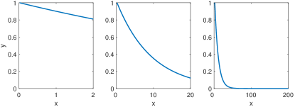
b

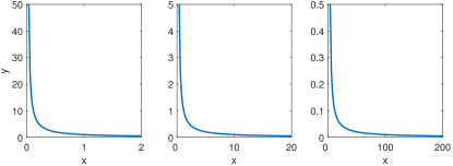
Figure 1: Exponential discounting introduces a scale; power-law discounting is scale-free. a. An exponential function has qualitatively different properties at different scales. The function $y=\gamma^{x}$ is shown at three different scales for $\gamma=0.9$. If $x$ is on the order of the time constant ($-\log\gamma$) we obtain the familiar exponential function with a clearly defined gradient for different values of $x$ (middle). If $x$ is small with respect to the time constant, we find a linear function with a shallow slope (left). If $x$ is large relative to the time constant (right), the function approximates a delta function with a peak around zero. b. Power-law discounting ($y=x^{-1}$). For all ranges of $x$ values the power law gives the same relative gradient of values.

1.2 Representing the future with a scalar obscures temporal information

One could implement scale-invariant power-law discounting by choosing an appropriate spectrum of exponential discount rates KurtEtal09; Sutt95. However it is computed, a discounted value discards potentially important information about when an anticipated event will occur. For instance, consider the decision facing an agent about whether to buy a cup of very hot coffee. Drinking the coffee immediately would burn one’s mouth. However, drinking the coffee after waiting a few minutes for it to cool down will result in a delicious and stimulating beverage. Is the value of the coffee negative (burned mouth) or positive (delicious beverage) or some weighted sum of the two? One way to answer the question is to state that the value of the coffee is a function over future time that is initially negative and then later positive. If the only information about this function that can be brought to bear in deciding whether to purchase the coffee is a single scalar value, then the decision-maker may choose an inappropriate action, either purchasing the coffee when she does not have time to wait for it to cool or missing the opportunity to enjoy a delicious beverage in the near future.

One could tackle this problem using model-free RL approaches by expanding the state space to include relevant variables, such as the elapsed time that the cup has been held and the steam coming from the cup. However, when the elapsed time is one of the variables that the agent needs to keep track of, this approach becomes computationally very expensive. This is because the number of states rapidly increases. If time is discretized into $m$ bins and we need to keep track of $n$ stimuli, then the number of states is $m^{n}$. This is especially costly when time is discretized in equal-sized bins as in complete serial compound representation. Using microstates characterized with a set of compressed temporal basis functions as in LudvEtal08; LudvEtal12 reduces the number of states to some degree, but this type of representation does not provide a future timeline.

Classical model-based RL enables decisions that take into account the time at which future events will take place. However the computational cost of traditional model-based solutions grows linearly with the horizon over which one needs to estimate the future. In this paper, we present a method that constructs a function over future time for each stimulus (state). This representation of the future is logarithmically compressed and the estimate of the future at many different points in time can be computed in parallel. One could compute an integral over this representation to maintain a cached value with power-law discounting. But because the entire function is available, an agent can also incorporate the time at which rewards will become available into its decision making.

1.3 Scale-invariant temporal representations in the brain

The basic computational strategy we pursue is to 1) compute a scale-invariant representation of the temporal history leading up to the present and 2) at each moment associate the history with the stimulus observed in the present. Step 1 assumes the existence of a scale-invariant compressed representation of temporal history. Step 2 assumes the existence of an associative mechanism. There is ample neural evidence for both of these assumptions. A large literature from the cellular neuroscience literature provides evidence for an associative mechanism implementing Hebbian plasticity at synapses BlisColl93; LismEtal02, which would be required for Step 2.

There is also a growing body of evidence consistent with assumptions necessary for Step 1. Experiments from several species suggest that the brain maintains a compressed representation of time in multiple brain regions. “Time cells” fire during a circumscribed period of time within a delay interval PastEtal08; MacDEtal11; a reliable sequence of time cells tile the delay on each trial (Figure 5a). Because the sequence is reliable, time cells can be used to reconstruct how long in the past the delay began. In many experiments, these sequences also carry information about what stimulus initiated the delay interval PastEtal08; MacDEtal13; TigaEtal18a; TeraEtal17. Because there are fewer cells that fire later in the sequence and those that fire later in the sequence fire for a longer duration HowaEtal15; SalzEtal16, the ability to reconstruct time decreases as the start of the interval recedes into the past. Time cells have been observed in several brain regions, including hippocampus MacDEtal11; SalzEtal16, prefrontal cortex TigaEtal16; BolkEtal17; TigaEtal18a and striatum MellEtal15; AkhlEtal16, in several species MauEtal18; AdleEtal12; TigaEtal18a and in a wide variety of behavioral tasks.

Taken together, these data indicate that at each moment the brain maintains a temporal record of what happened when leading up to the present. The decrease in accuracy for events further in the past suggests that this temporal record is compressed. As such, this neural data aligns with longstanding predictions from cognitive models BrowEtal07; BalsGall09; HowaEtal15. These models further predict that the form of compression should be logarithmic. Behavioral models built from a logarithmically-compressed representation readily account for scale-invariant behavior HowaEtal15.

1.4 Overview of this paper

In this paper we use a logarithmically-compressed record of the past—a set of appropriate time cells—to construct a scale-invariant estimate of the time of future events. A logarithmically-compressed record of the past can be efficiently computed using a method we will describe in detail below ShanHowa12; ShanHowa13. At each moment, this representation of the past is associated to the present. Neurally, this association requires nothing more elaborate than Hebbian plasticity, which can be implemented via long-term potentiation BlisColl93. The past-to-present association can also be understood as a present-to-future association. As such, multiplying this association with the present stimulus vector enables us to identify the sequence of stimuli that will follow the probe stimulus at different points in the future. Section 2 describes this method more precisely.

This method yields an estimate of the future that has very different properties than traditional approaches used in RL. The properties of this representation are described with illustrative examples in Section 3. Because the representation of the past is logarithmically compressed, so too is the estimate of the future that it produces. A cached scalar value can be computed from this timeline, yielding (scale-invariant) power-law discounting by summing over the predicted future. Notably, the compressed timeline representation also provides a function over simulated time. The future timeline can be computed in a single parallel operation and sums over potential outcomes. Section 4 describes neural and behavioral predictions of the model, reviewing recent empirical results that are consistent with the proposed hypothesis that the brain constructs a logarithmically compressed future.

2 Constructing a logarithmically-compressed timeline of the future

This approach requires two key components, a logarithmically-compressed memory representation and an associative memory between the compressed representation and the present stimulus. Subsection 2.1 describes a method for constructing a logarithmically-compressed memory representation following ShanHowa13. Subsection 2.2 describes the associative memory. Subsection 2.3 describes the future timeline that results from probing the associative memory with a stimulus representation.

2.1 Previous work: Constructing a compressed memory representation of the past

Consider a case in which the network is presented with a vector-valued input that changes over time $\mathbf{f}(t)$. This input reflects the presence or absence of a set of discrete stimuli (states) that we denote as $I={\alpha,\ \beta,\ \gamma\ldots}$. For simplicity, let us assume that the input uses a localist (one-hot) representation; if stimulus $\alpha$ is present at time $t$ we write $f_{\alpha}(t)=1$. Now, the goal of this method is to construct an estimate of the past leading up to the present. We refer to this memory representation as $\tilde{\mathbf{f}}$. A temporal record of the past requires two types of information. In order to estimate $\mathbf{f}(t^{\prime}<t)$ we need to maintain both what and when information. Thus, we index each of the neurons in $\tilde{\mathbf{f}}$ by two indices, $\tilde{f}_{\overset{*}{\tau},i}$ (Figure 2). The second index $i\in I$ corresponds to the what information. The other index, $\overset{*}{\tau}$ refers to the time in the past that this neuron is attempting to represent. That is, the network includes a set of values of $\overset{*}{\tau}\in\{\overset{*}{\tau}_{1},\ \overset{*}{\tau}_{2},\ \overset{*}{\tau}_{3}$ …$\}$. Because the value of $\overset{*}{\tau}$ for the $i$th row of the network, $\overset{*}{\tau}_{i}$ has physical meaning, we refer to the neurons in $\tilde{\mathbf{f}}$ by their value of $\overset{*}{\tau}$ rather than their row number. Each entry $\tilde{f}_{\overset{*}{\tau},\alpha}(t)$ approximates $f_{\alpha}(t+\overset{*}{\tau})$. Here the values of $\overset{*}{\tau}$ are negative as they refer to a temporal distance in the past relative to the present.

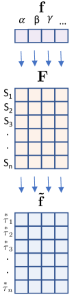
Figure 2: Constructing a memory representation of the recent past. The schematic shows the two-layer network for constructing a memory representation by implementing an approximation of the Laplace and the inverse Laplace transform. The input $\mathbf{f}$ is a vector over states $\alpha$, $\beta$, $\gamma$… This provides input to a two-layer network where each layer is a 2-D array (sheet) of neurons. Neurons in the first layer $\mathbf{F}$ are leaky integrators indexed by the state they encode, $\alpha$, $\beta$, $\gamma$… and their rate constant $s$. We refer to the activation of a particular entry as $F_{s,\alpha}$. Neurons in the second layer $\tilde{\mathbf{f}}$ activate sequentially following the input stimulus. They are indexed by the state that provides their input and the time by which the peak of their activation follows the input stimulus $\overset{*}{\tau}$. The activation of a particular unit is referred to as $\tilde{f}_{\overset{*}{\tau},\alpha}$.

a

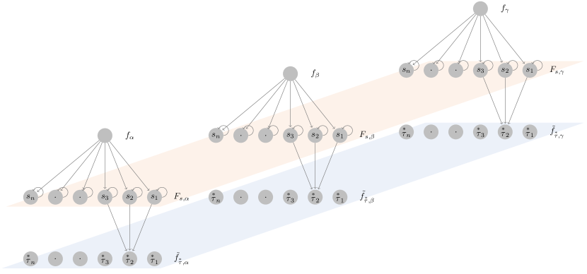
b	c

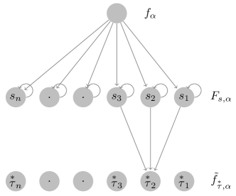
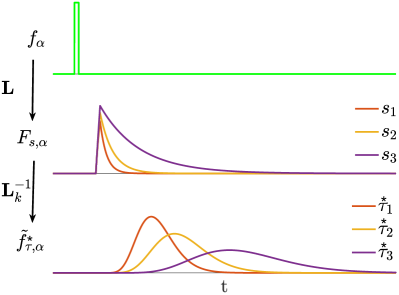
Figure 3: Structure and dynamics of the memory representation. a. The two-layer network is organized such that each input state has its own set of units in $\mathbf{F}$ and $\tilde{\mathbf{f}}$ layers (when constructing the memory representation, there is no crosstalk between the neurons that correspond to different states). b. The input stimulus $f_{\alpha}(t)$ feeds into a layer of leaky integrators $F_{s,\alpha}$ that implement a discrete approximation of an integral transform. Each neuron in the first layer has a characteristic rate constant $s_{i}$. $F_{s,\alpha}$ projects onto $\tilde{f}_{\overset{*}{\tau},\alpha}$ through a set of weights defined with the operator $\mathbf{L}^{\textrm{\scriptsize{-1}}}_{k}$ which implements an approximation of the inverse of the Laplace transform. Notice that the $\mathbf{L}^{\textrm{\scriptsize{-1}}}_{k}$ operator projects only to a local neighborhood ($k$ neurons). Neurons in the second layer each have their characteristic peak time relative to the input onset $\overset{*}{\tau}_{i}$. Analytic relationship between $\overset{*}{\tau}$ and $s$ can be expressed as $\overset{*}{\tau}=-k/s$. Thus choosing $\overset{*}{\tau}$ and integer $k$ fully specifies $s$, similarly, choosing $s$ and $k$ fully specifies $\overset{*}{\tau}$. We chose $\overset{*}{\tau}$ to be logarithmically spaced (in order to have a logarithmically compressed memory representation). c. A response of the network to a delta-function input. Activity of only three neurons in each layer is shown. Neurons in $\tilde{f}_{\overset{*}{\tau},\alpha}$ activate sequentially following the stimulus presentation. The width of the activation of each neuron scales with the peak time determined by the corresponding $\overset{*}{\tau}$, making the memory scale-invariant.

Following prior work ShanHowa12; ShanHowa13 we will construct the representation of the past $\tilde{\mathbf{f}}$ by means of an intermediate representation $\mathbf{F}$. Each neuron in $\mathbf{F}$ aligns with a corresponding neuron in $\tilde{\mathbf{f}}$ (Figure 3a). The neurons in $\mathbf{F}$ are indexed by the label of the stimulus in the world that activates them ($\alpha,\ \beta,\ \gamma\ \ldots$) and a scalar value $s$. The values of $s$ for each row of $\mathbf{F}$ align with the corresponding values of $\overset{*}{\tau}$ in each row of $\tilde{\mathbf{f}}$ (Figure 3b):

$$F_{s,\alpha}\leftrightarrow\tilde{f}_{\overset{*}{\tau},\alpha}.$$ (2)

The mapping between $s$ and $\overset{*}{\tau}$ is such that $s=-k/\overset{*}{\tau}$ , where $k$ is an integer with physical meaning that will be described below and $i\in 1,2,3\ldots n$, where $n$ is the number of rows in $\mathbf{F}$ and $\tilde{\mathbf{f}}$. As with $\overset{*}{\tau}$, there are a finite set of values of $s$, $s\in\{s_{1},\ s_{2},\ s_{3}$ …$\}$. As with $\overset{*}{\tau}$, there is a physical meaning to the $i$th value of $s$ so we refer to neurons in $\mathbf{F}$ by their value of $s_{i}$ rather than their index $i$. Values of $s$ are defined to be positive. Following previous work ShanHowa13; HowaShan18, we choose the values of $\overset{*}{\tau}$ and $s$ to be evenly spaced on a logarithmic scale.

The dynamics of each unit in $\mathbf{F}$ obeys:

$$\frac{dF_{s,\alpha}(t)}{dt}=-sF_{s,\alpha}(t)+{f}_{\alpha}(t),$$ (3)

where the value of $s$ on the rhs refers to that particular neuron’s value $s_{i}$. Here we can see that $s$ describes each neuron’s rate constant; $1/s$ describes each neuron’s time constant. Taking the network state across all values of $s$, $\mathbf{F}(s)$ estimates the Laplace transform of $\mathbf{f}(t^{\prime}<t)$. To see that $F_{s,\alpha}$ at time $t$ is the Laplace transform of $f_{\alpha}(t^{\prime}<t)$, solve Eq. 3:

$$F_{s,\alpha}(t)=\int_{-\infty}^{t}e^{-s\left(t-t^{\prime}\right)}f_{\alpha}(t^{\prime})dt^{\prime}.$$ (4)

Knowing that $\mathbf{F}$ at time $t$ holds the Laplace transform of $\mathbf{f}$ leading up to the present suggests a strategy to construct an estimate of $\mathbf{f}$. If we could invert the transform and write the answer into another set of neurons $\tilde{\mathbf{f}}$, this would provide an estimate of $\mathbf{f}$ as a function of time leading up to the present. The Post approximation Post30 provides a recipe for approximating the inverse transform that can be computed with a set of feedforward weights, which we denote $\mathbf{L}^{\textrm{\scriptsize{-1}}}_{k}$:

$$\tilde{f}_{\overset{*}{\tau},\alpha}(t)=\mathbf{L}^{\textrm{\scriptsize{-1}}}_{k}F_{s,\alpha}(t).$$ (5)

The integer $k$ determines the precision of the approximation. Denoting the $k^{th}$ derivative with respect to $s$ as $F^{(k)}_{s,\alpha}$ we can rewrite Eq. 5 as:

$$\tilde{f}_{\overset{*}{\tau},\alpha}(t)=C_{k}s^{k+1}F^{(k)}_{s,\alpha}(t),$$ (6)

where $C_{k}$ is a constant that depends only on $k$.

To get an intuition into the properties of $\tilde{f}$, we present a delta function to $f_{\alpha}$ at time zero and examine the activity of $F_{s,\alpha}(t)$ and $\tilde{f}_{\overset{*}{\tau},\alpha}(t)$. We find immediately that $F_{s,\alpha}(t)=e^{-st}$. Moreover, the activity of the neurons in $\tilde{\mathbf{f}}$ obeys:

$$\tilde{f}_{\overset{*}{\tau},\alpha}(t)=C_{k}\frac{1}{\overset{*}{\tau}}\left(\frac{t}{\overset{*}{\tau}}\right)^{k}e^{-k\frac{t}{\overset{*}{\tau}}},$$ (7)

where $C_{k}$ here is a different constant that depends only on $k$. The activity of each node in $\tilde{f}_{\overset{*}{\tau},\alpha}$ is the product of an increasing power term $\left(\frac{t}{\overset{*}{\tau}}\right)^{k}$ and a decreasing exponential term $e^{-k\frac{t}{\overset{*}{\tau}}}$. In the time following a delta function input, the firing of each neuron in $\tilde{f}_{\overset{*}{\tau},\alpha}$ peaks at $\overset{*}{\tau}$ (Figure 3c). Thus, following a transient input of state $\alpha$, neurons in $\tilde{f}_{\overset{*}{\tau},\alpha}$ activate sequentially.

Figure 4a shows the sequential, spreading activation with logarithmically spaced $\overset{*}{\tau}$ for three different transient stimuli. This mathematical model for estimating the past has properties that resemble sequentially activated time cells <compare to Fig. 5; see also>HowaEtal14,TigaEtal18a. Previous biophysical modeling has developed a neurally plausible mechanism for implementing leaky integrators with a spectrum of time constants TigaEtal15 and for constructing a circuit implementing the inverse transform LiuEtal18.

a	b

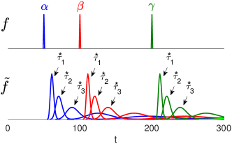
Figure 4: Constructing an associative memory by building connections between present inputs and memory of the recent past. a. Illustration of the compressed memory representation $\tilde{\mathbf{f}}$ as a function of time during presentation of the sequence $\alpha$, $\beta$, $\gamma$. Stimuli presented at different times (top) induce sequential activation (bottom) in $\tilde{\mathbf{f}}$. Activation corresponding to different stimuli is shown with different colors. For clarity, only a handful of neurons are displayed. b. A graphical depiction of the state of the associative memory $\mathbf{M}$ after learning of the sequence $\alpha$, $\beta$, $\gamma$. Each of the three plots shows entries stored in $\mathbf{M}$ as a function of $\overset{*}{\tau}$. $\mathbf{M}_{\overset{*}{\tau},q,r}$ is the synaptic weight from $r$ to $q$ at a particular $\overset{*}{\tau}$. The different stimuli are shown in different colors in each plot. Top: Associations stored in $M_{\overset{*}{\tau},\gamma,\alpha}$, $M_{\overset{*}{\tau},\gamma,\beta}$ and $M_{\overset{*}{\tau},\gamma,\gamma}$ as functions of log-spaced $\overset{*}{\tau}$. Because $\gamma$ was preceded by both $\alpha$ and $\beta$, both $M_{\overset{*}{\tau},\gamma,\alpha}$ and $M_{\overset{*}{\tau},\gamma,\beta}$ have peaks. Because $\beta$ had been presented more recently when $\gamma$ was presented, the curve for $M_{\overset{*}{\tau},\gamma,\beta}$ has a peak closer to $\overset{*}{\tau}=0$. Because the representation of times in the more recent past is more accurate than times further in the past, the peak for $\beta$ is also more sharp as a function of $\overset{*}{\tau}$. Middle: Associations stored in $M_{\overset{*}{\tau},\beta,\alpha}$, $M_{\overset{*}{\tau},\beta,\beta}$ and $M_{\overset{*}{\tau},\beta,\gamma}$. Because $\beta$ was preceded by $\alpha$ at a short lag, $M_{\overset{*}{\tau},\beta,\alpha}$ differs from zero at low values of $\overset{*}{\tau}$. Since $\beta$ was not preceded by itself or by $\gamma$, blue and green traces are zero. Bottom: Associations stored in $M_{\overset{*}{\tau},\alpha,\alpha}$, $M_{\overset{*}{\tau},\alpha,\beta}$ and $M_{\overset{*}{\tau},\alpha,\gamma}$. Since $\alpha$ was not preceded by any stimulus, corresponding entries in $\mathbf{M}$ are zero for all values of $\overset{*}{\tau}$.

a
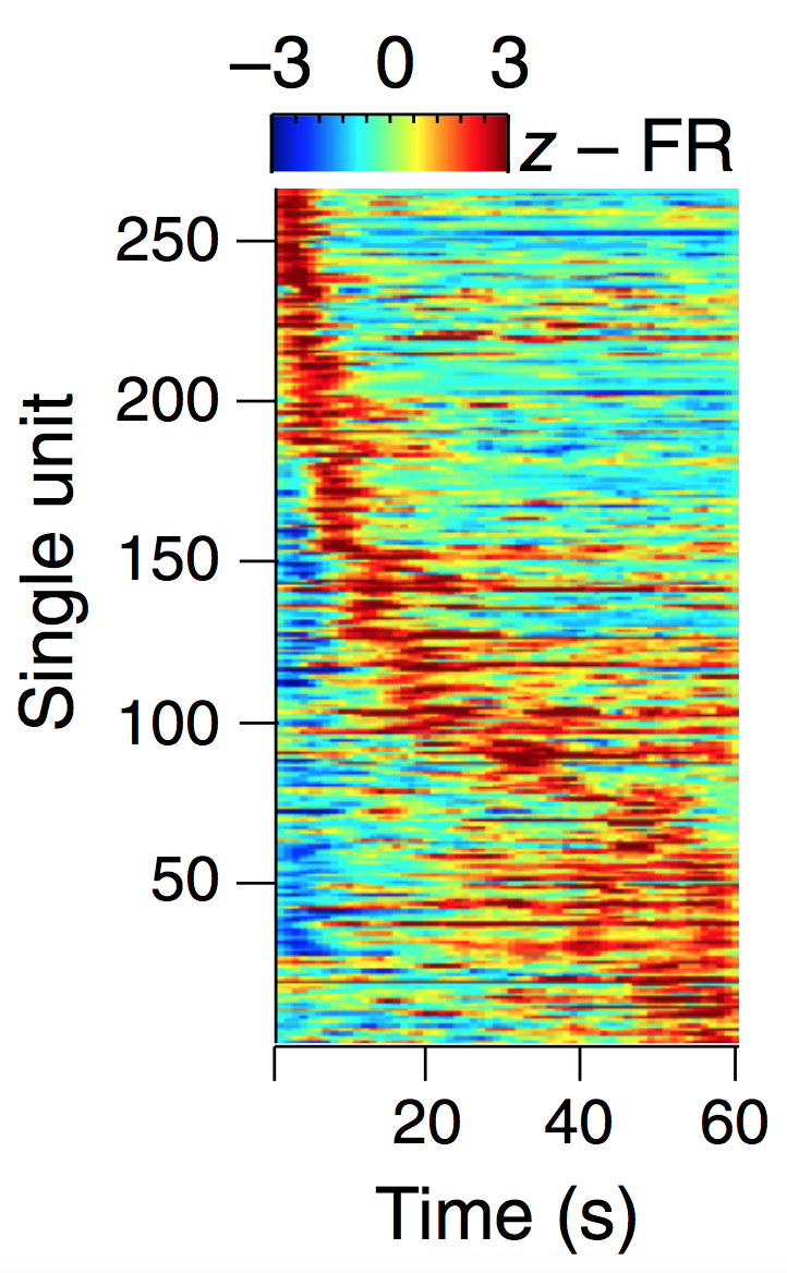
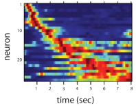
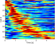
b

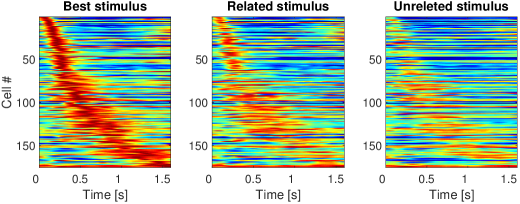
Figure 5: Recordings of sequentially-activated time cells in different behavioral tasks, different mammalian species and different brain regions. a. Sequences of time cells in the brain contain information about the time of past events. Each of the four plots shows the activity of many neurons during the delay period of a behavioral task. In each plot each row gives the average firing rate as a function of time for one neuron. Red colors indicate a high firing rate. Because neurons fire for a circumscribed period of time during the delay, these neurons could be used to decode the time at which the delay started. Put another way, each neuron can be understood as coding for the presence of the start of the delay at a lag $\overset{*}{\tau}$ in the past. The number of cells active at any one time decreases as the delay unfolds (note the curvature) and the firing fields spread (note the increasing width of the central ridge). This reflects a decrease in accuracy for time as the start of the delay recedes further into the past. From left to right: mouse mPFC during a spatial working memory task, after Bolkan et al., 2017; rat hippocampus, during the delay period of a working memory task, after MacDonald et al., 2011; rat mPFC during a delay period of temporal discrimination task, after Tiganj et al., 2016. b. Sequentially activated cells in monkey lPFC encode time conjunctively with stimulus identity during delayed-match-to-category task. Animals were presented with stimuli chosen from four categories (dogs, cats, sports cars and sedan cars). Based on visual similarity the stimuli belonged to two category sets (animals and cars). The time interval shown on the plots includes 0.6 s sample stimulus presentation and 1 s delay interval that followed the sample stimulus. Each of the three heatmaps shows the response of every unit classified as a time cell. The units show distinct firing rate for different stimuli that started the delay interval, reflecting the visual similarity (magnitude of the response for Related stimulus was larger than for Unrelated stimulus) and indicating stimulus selectivity of time cells. After Tiganj et al., 2018.

$\tilde{\mathbf{f}}$ approximates $\mathbf{f}$ leading up to the present. However, the precision of the approximation decreases for events further in the past. One way to see this is that the duration over which $\tilde{f}_{\overset{*}{\tau},\alpha}$ is activated by a delta function input increases as one chooses larger values of $|\overset{*}{\tau}|$. However, this inaccuracy is scale invariant; the spread in time for a neuron with a particular $\overset{*}{\tau}$ is a rescaled version of the firing of another neuron that received the same input but has a different value of $\overset{*}{\tau}$. Put another way, the activity of every neuron receiving a delta function input obeys the same time dependence in units of $t/|\overset{*}{\tau}|$. This rescaling of the activity of neural response in time also has a correspondence in the pattern of activity across neurons with different values of $\overset{*}{\tau}$ as the stimulus recedes into the past. At any moment, when the stimulus is $t_{o}$ time in the past, there is a bump of activity centered around the neurons with $\overset{*}{\tau}\simeq t_{o}$. However, the difference in the value of $\overset{*}{\tau}$ between adjacent neurons is not constant (for instance note the increasingly spread points in Figure 4b). With logarithmic spacing of $\overset{*}{\tau}$ values, the shape of the bump of activity across neuron number remains of constant width as the stimulus recedes into the past HowaEtal15.

2.2 Constructing an associative memory

At each time $t$, an associative memory tensor $\mathbf{M}$ is updated with the outer product of the current input state $\mathbf{f}$ and $\tilde{\mathbf{f}}$ (Figure 4b). Hence $\mathbf{M}$ is a three-tensor. At each moment, $\mathbf{M}$ is updated with the simple Hebbian learning rule:

$$\frac{d{M}_{\overset{*}{\tau},\beta,\alpha}}{dt}=\lambda\ {f}_{\beta}(t)\ \tilde{f}_{\overset{*}{\tau},\alpha}(t).$$ (8)

Here $\lambda$ is a learning rate that we choose to be 1. $\mathbf{M}$ can be implemented as set of synaptic weights learned through Hebbian plasticity. Because $\tilde{\mathbf{f}}_{\overset{*}{\tau},\alpha}$ stores a coarse-grained estimate of the past, its average over many experiences, $\mathbf{M}$, is a coarse-grained estimate of the lagged cooccurrence of each pair of states:

$$M_{\overset{*}{\tau},\beta,\alpha}\propto P\left[\textbf{f}(t+|\overset{*}{\tau}|)=\beta,\ \ \textbf{f}(t)=\alpha\right],$$ (9)

where $P$ denotes probability.

We can also construct an estimate of the conditional probability by normalizing $\mathbf{M}$ as follows:

$$\bar{M}_{\overset{*}{\tau},\beta,\alpha}\equiv\frac{{M}_{\overset{*}{\tau},\beta,\alpha}}{\sum_{i\in I}{M}_{\overset{*}{\tau},\beta,i}}.$$ (10)

One could imagine that this normalization is implemented on-line by a divisive presynaptic normalization mechanism BeckEtal11. Now $\bar{\mathbf{M}}$ is an associative memory that provides a coarse-grained estimate of the conditional probability of state $\beta$ following state $\alpha$ at a lag of $|\overset{*}{\tau}|$:

$$\bar{M}_{\overset{*}{\tau},\beta,\alpha}\propto P\left[\textbf{f}(t+|\overset{*}{\tau}|)=\beta\ |\ \textbf{f}(t)=\alpha\right].$$ (11)

As we will see in the next subsection, by multiplying $\bar{\mathbf{M}}$ from the right with a current state, we can generate the probability of all other states following at each possible lag.

2.3 Estimating a future timeline

$\mathbf{M}$ stores the pairwise temporal relationships between all stimuli subject to logarithmic compression. At the moment a state is experienced, the history leading up to that state is stored in $\mathbf{M}$ (eq. 8). After many presentations, $\mathbf{M}$ records the probability that each state is preceded by every other state at each possible lag. This record of the past can also be used to predict the future. By multiplying $\bar{\mathbf{M}}$ with the current state from the right we can generate an estimate of the future. In a general case, let us consider $\mathbf{f}(t)$ that can have multiple stimuli presented at the same time. Stimuli that will follow the present input $\mathbf{f}(t)$ at a time lag $|\overset{*}{\tau}|$ can be estimated from the information recorded in $\bar{\mathbf{M}}$:

$$\mathbf{p}_{-\overset{*}{\tau}} \equiv \bar{\mathbf{M}}_{\overset{*}{\tau}}\mathbf{f}$$ (12)

$${p}_{-\overset{*}{\tau},\beta} = \sum_{i\in I}\bar{M}_{\overset{*}{\tau},\beta,i}f_{i}.$$ (13)

Like $\mathbf{F}$ and $\tilde{\mathbf{f}}$, $\mathbf{p}$ can be understood as a 2-D array indexed by stimulus identity and $\overset{*}{\tau}$. However, whereas for $\tilde{\mathbf{f}}$, $\overset{*}{\tau}$ is negative corresponding to estimates of the past, for $\mathbf{p}$ the values of $\overset{*}{\tau}$ are positive, corresponding to estimates of the future. The value of $\overset{*}{\tau}$ for the $i$th row of $\tilde{\mathbf{f}}$ and the value of $\overset{*}{\tau}$ for the $i$th row of $\mathbf{p}$ have the same magnitude but are opposite in sign. ${p}_{-\overset{*}{\tau},\beta}$ is a magnitude of the prediction that state $\beta$ will follow present input $\mathbf{f}$ at a time lag $|\overset{*}{\tau}|$. When the input is interpretable as a probability density function (when $\sum|\mathbf{f}|=1$), then $\mathbf{p}_{-\overset{*}{\tau}}$ is also a probability density function. When $\mathbf{f}$ is not a probability density function, $\mathbf{p}_{-\overset{*}{\tau}}$ is not either.

In a more specific case, when $\mathbf{f}(t)$ can have only one stimulus presented at the same time, magnitude of the prediction that state $\beta$ will follow the present input, say state $\alpha$, at a time lag $|\overset{*}{\tau}|$ is a scalar stored in $\bar{M}_{\overset{*}{\tau},\beta,\alpha}$:

$${p}^{\alpha}_{-\overset{*}{\tau},\beta} = \bar{M}_{\overset{*}{\tau},\beta,\alpha}.$$ (14)

Note that $\mathbf{p}^{\alpha}$ inherits the same compression present in $\tilde{\mathbf{f}}$. The “blur” in the estimate of the time of presentation of a past stimulus in $\tilde{\mathbf{f}}$ with $\overset{*}{\tau}<0$ naturally leads to an analogous blur in $\mathbf{p}^{\alpha}$ as a function of future time $\overset{*}{\tau}>0$. Expected future outcome at a lag $\overset{*}{\tau}$ can be estimated by examining the states predicted at that lag and estimating the reward status of each. Properties of this representation of future time are illustrated in more detail in Section 3.

3 Illustrating the properties of the representation of future time

In this section we illustrate properties of the representation of future time constructed by multiplying $\bar{\mathbf{M}}$ with a particular state vector (Eq. 14). In subsection 3.1 we demonstrate that the representation that results is scale-invariant. In subsection 3.2 we show that a cached value for each state can be computed, resulting in a scale-invariant value that is discounted according to a power law. In subsection 3.3 we illustrate the flexibility of this method in generating non-monotonic functions enabling the user to solve problems such as the “hot coffee” problem described in the introduction. In subsection 3.4 we demonstrate that future time gives an estimate summed over all possible paths. Finally, in subsection 3.5 we demonstrate application of this approach in decision making.

3.1 Scale-invariance of future time

If two environments differ only in their temporal scale, an artificial agent based on a scale-invariant algorithm will take the same actions in both environments. This property is illustrated for this method through a simple toy example in Figure 6. In this example, there are two states to choose from, $\alpha$ and $\beta$, and a third rewarding state r that the agent is interested in predicting. The two environments shown in Figure 6 differ only in the temporal spacing between different stimuli. The bottom environment (marked as Scale 4, Figure 6b) is a temporally stretched version of the top environment (marked as Scale 1, Figure 6a). Stretching the time axis of the top environment by 4 times would give exactly the bottom environment. At the decision point $D$ at time $t=0$ the agent needs to choose either state $\alpha$ or state $\beta$ (the example is designed as a deterministic Markov decision process so taking an action can be understood as directly selecting a state).

Under the assumption that the agent has explored the environment by choosing each direction at least once, all needed temporal associations are stored in $\bar{\mathbf{M}}$. Next time when the agent faces the decision point at time $t=0$ it can construct the future time as in Eq. 14. The predictions $\mathbf{p}^{\alpha}$ and $\mathbf{p}^{\beta}$ constructed separately for $\alpha$ and $\beta$ both give power-law discounted estimates of the expected future outcome that rescale with rescaling of the environment.

a
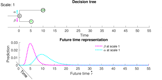
b

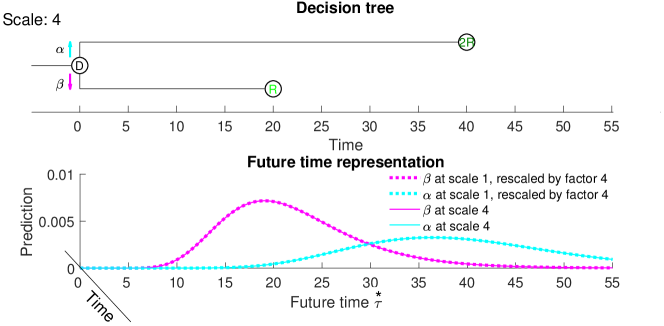
Figure 6: The representation of future time is scale-invariant. In this and subsequent figures, the agent evaluates the degree to which each of two states, $\alpha$ and $\beta$, predict a desired outcome r. The decision tree in the environment is shown in the top panel. The estimate of the future cued by each of the two states $\alpha$ and $\beta$ as a function of future time $\overset{*}{\tau}$ is shown by the lines at the bottom. a. A simple decision tree in which $\alpha$ predicts reward after 5 units of time and $\beta$ predicts reward after 10 units of time. The dashed lines show that the cues predict reward at different times. Note that the prediction of events further in the future is made with less precision. (The reward predicted by $\beta$ is twice the size of the reward predicted by $\alpha$ to make the figure easier to read.) b. The same decision tree, but with the temporal intervals rescaled by a factor of 4. The solid lines show the predictions from the environment in a rescaled by a factor of 4 (i.e., stretched by a factor of 4 and multiplied by 4). Note that the functions in the two environments are precisely rescaled versions of one another.

3.2 Computing cached power-law discounted stimulus value by integrating over the timeline

There are circumstances where a decision-maker does not have time to evaluate a compressed function over future time and a cached value of each state would be sufficient. A cached value can be computed by maintaining, for each state, an average value over future time updated by taking an integral over the future:

$$V^{\alpha}(t)=\sum_{i\in I}r_{i}\int_{0}^{\infty}p^{\alpha}_{\overset{*}{\tau},i}\ g_{\overset{*}{\tau}}\ d\overset{*}{\tau},$$ (15)

where $\mathbf{r}$ is a column vector describing the value of each state and $g_{\overset{*}{\tau}}$ is the number density of $\overset{*}{\tau}$ values $\frac{dN}{d\overset{*}{\tau}}$. The number density $g_{\overset{*}{\tau}}=dN/d\overset{*}{\tau}$ specifies how many units are used to represent a particular spacing of $\overset{*}{\tau}$. For instance, if spacing between $\overset{*}{\tau}$ nodes would be linear the number density $g_{\overset{*}{\tau}}$ would be 1. With logarithmic spacing of $\overset{*}{\tau}$ the number density goes down as $1/\overset{*}{\tau}$.

In order to ensure Weber-Fechner spacing, we here set $g_{\overset{*}{\tau}}={\overset{*}{\tau}}^{-1}$, but one could in general augment this by including a function to differentially weight the contribution of different values of $\overset{*}{\tau}$. As long as that function does not introduce a scale, the cached value computed in this way will remain scale invariant (power-law). Figure 7 illustrates properties of value computed from Eq. 15.

Applying Eq. 15 to the example shown in Figure 6 reveals that the ratio of the values for states $\alpha$ and $\beta$ is constant when time is rescaled. This means that the relative values assigned to various choices do not depend on the time-scale of the environment, but only on their relative magnitude and timing.

a		b		c

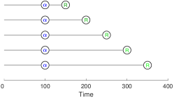
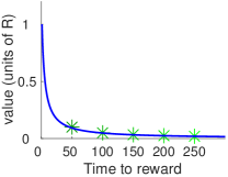
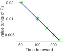
Figure 7: The value aggregated by integrating over future time obeys power-law discounting. a. Constructing prediction of the future reward. An agent observed a temporal sequence consisting of a state $\alpha$, followed by a rewarding state R at some delay. b. The value of $\alpha$ computed according to Eq. 15 as a function of the delay between $\alpha$ and reward (expressed in the units of the reward $R$). The value associated with the five evenly spaced delays in a are shown as star symbols. The blue line is a power law with exponent $-1$. c. Same as b but on log-log axes.

3.3 Non-monotonic functions over future time

In traditional RL, the value of each state is a scalar. The approach introduced here provides a recipe for simulating a function of a logarithmically compressed future. The example in Figure 8 illustrates one case in which this type of representation has an advantage over the scalar representation. In this example state $\alpha$ is neutral; no meaningful outcome follows it. However, state $\beta$ is followed sequentially by a negative outcome (e.g., a burned mouth) and then later by a positive outcome (e.g., delicious coffee). The ability to simulate outcomes as a function of future time can enable the agent to make decisions in a more flexible way (by dynamically altering the time horizon of planning) than would be possible if all the available information about the future was expressed as a scalar.

Notice that the same amount of information is conveyed even when having only the set of exponentially decaying neurons ($\mathbf{F}$ neurons). However, applying the inverse Laplace transform and estimating the future as proposed here allows the agent to examine the future directly in the units of time, without need for an additional decoder. This type of representations provides direct access to temporal order and distance. In general, coding with bell-shaped turning curves appears to be widely used in the brain with place cells in the hippocampus, angle selective cells in visual and motor areas being some of well known examples.

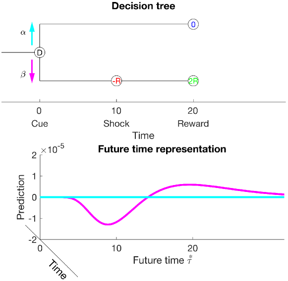
Figure 8: The estimate of a future timeline enables the decision-maker to anticipate different outcomes at different points in time. Top: Choice $\alpha$ is neutral, predicting neither reward nor punishment. Choice $\beta$ results in a negative outcome (e.g., a shock) after 10 units of time and then a large positive outcome after 20 units of time. Bottom: The representation of future time induced by each choice varies as a function of the temporal horizon. $\alpha$ is preferable to $\beta$ at short delays but $\beta$ is preferable to $\alpha$ at longer delays. A decision-maker could incorporate this information about the future time course when the choices are presented.

3.4 Future time sums over trajectories

Figure 9 illustrates an important property of the proposed approach: simulated future time provides a probability of each stimulus $\overset{*}{\tau}$ in the future summed across all possible future trajectories. Let us assume that the agent has sampled the environment sufficiently many times to learn the transition probabilities and the temporal dynamics of the environment, which are now stored in $\bar{\mathbf{M}}$. Now computing the prediction $\mathbf{p}^{\alpha}_{\overset{*}{\tau}}$ as in Eq. 14 provides an overall estimate of the reward averaged across all the future trajectories. However, it retains information about how far in the future those outcomes will be obtained. This property allows a rapid evaluation of different decision trees. Evaluating a particular sequence of outcomes that depend on sequential actions would still require supplementing this representation with a more traditional model-based approach. Moreover, correctly learning the outcomes requires sampling the entire tree, which may be much slower than TD-based learning in an environment with Markov statistics.

Notice that in many problems in RL states that follow the present state often change in response to the action taken by the agent. For simplicity we are studying the Pavlovian case (similar to previous authors like SchuEtal97). In the control setting, we would need to simultaneously estimate M and a policy, since these are coupled. We think the interplay between prediction and control are very important and we leave that to future work.

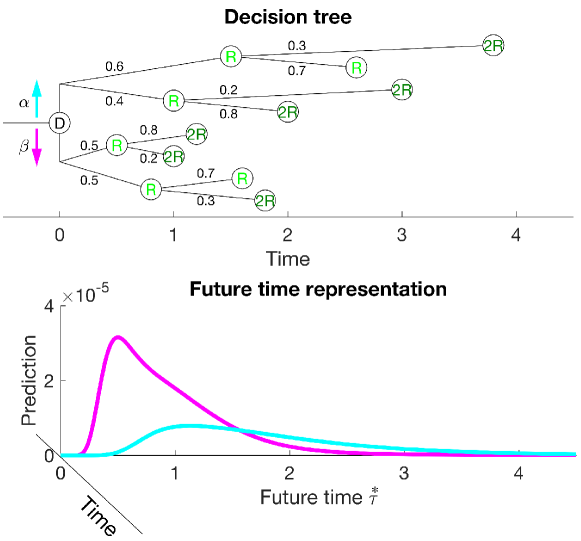
Figure 9: The estimate of a future timeline sums over all possible future trajectories. Top: The decision tree for a complex choice. Both $\alpha$ and $\beta$ lead to a complex set of possible outcomes that occur at specific times with given probabilities (shown as numbers near each branch of the tree). Bottom: The estimate of a future timeline averages over different possible paths with each outcome weighted by its probability of occurrence given the choice stimulus ($\alpha$ or $\beta$).

3.5 Temporally flexible decision making

The ability to construct a timeline of the future events enables flexible decision making that incorporates the decision-maker’s temporal constraints. For instance, consider making a decision about what to get for lunch while waiting for a train. The food option one pursues may be very different if one has 15 minutes before the train arrives than if one has an hour before the train arrives. Because the model carries separate information about when outcomes will be available as well as their identity it is possible to make decisions that differentially weight outcomes at different points in the future. If the decision-maker has a temporal window over which outcomes are valuable, $w_{\overset{*}{\tau}}$, then one can readily compute value using a generalization of Eq. 15:

$$V^{\alpha}(t)=\sum_{i\in I}r_{i}\int_{0}^{\infty}p^{\alpha}_{\overset{*}{\tau},i}w_{\overset{*}{\tau}}\ g_{\overset{*}{\tau}}\ d\overset{*}{\tau},$$ (16)

Figure 10 illustrates this capability. In this example, the model is presented with two alternatives that predict a valuable outcome but with different magnitude and different time course. When the decision-maker approaches the choice with a narrow temporal window, as in the case where the train will arrive in 15 minutes, choice a is more valuable. However, when choosing using a broader temporal window, as in the case where the train will arrive in one hour, choice b is more valuable.

A temporal representation of the future enables not only decision-making with different temporal horizons, but also decision-making based on relatively complex temporal demands. Consider the case where an outcome is not valuable in the immediate future, but only becomes valuable after some time has passed—for instance perhaps one is not hungry now but will be hungry in one hour. These capabilities are comparable to those offered by model-based RL. However, as discussed above, the representation of the future is scale-invariant and can be computed rapidly.

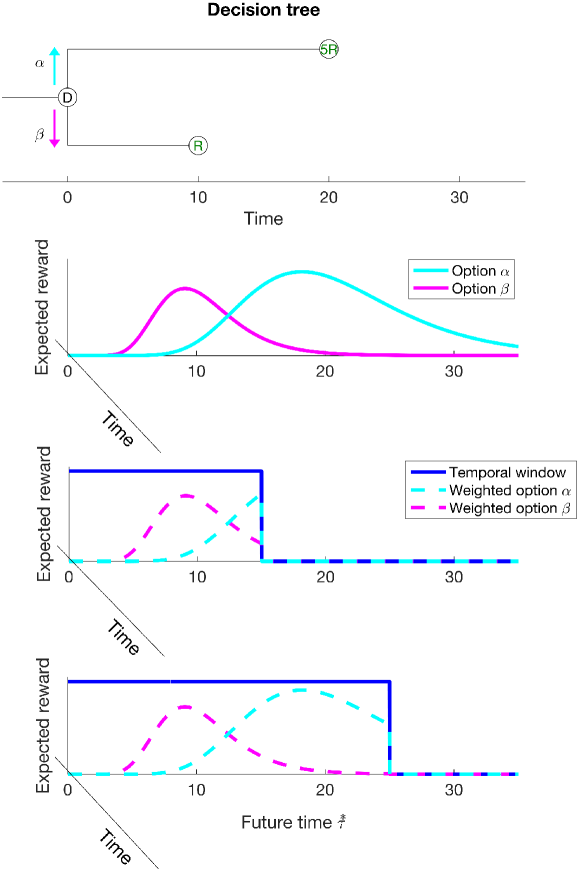
Figure 10: Temporally flexible decision making. Consider an agent faced with two options $\alpha$ and $\beta$ that differ in the time course over which they predict reward (top). Note that $\beta$ (magenta) predicts a larger reward, but further in the future, than does $\alpha$ (cyan). Representing a function over future time enables the agent to make decisions that incorporate information about the value of the outcome to the agent as a function of time. For instance, under some circumstances, an agent might have more or less time to exploit a food source before some other pressing engagement. The bottom two panels illustrate the value computation with each of two temporal windows. In the middle panel, the temporal window over which the agent can exploit the reward is narrow and the agent chooses $\alpha$. In the bottom panel, the temporal window extends further into the future and the agent chooses $\beta$.

4 Behavioral and neural predictions

Earlier sections presented a method for constructing a compressed estimate of the future. Because this approach is novel, there is not yet empirical data to definitively evaluate key predictions of this approach. In this section we describe neural and behavioral predictions and describe how those could be tested experimentally. We also point to recent empirical results, both behavioral and neural, that support the proposed hypothesis, albeit obliquely.

4.1 Cognitive scanning of the future

This paper proposes a neural mechanism for constructing a compressed representation of the future. In the cognitive psychology of working memory, prior findings from the short-term judgment of recency (JOR) task suggest that people can scan a compressed representation of the past. For instance, Hack80 presented participants a series of letters rapidly and asked them to evaluate which of two probes was experienced more recently. The critical finding was that the time to choose a probe depended on how far in the past that probe was presented and did not depend on the recency of the other probe. These findings suggested that participants sequentially examine a temporally-organized representation of the past and terminate the search when they find a target <see also>Mute79,Hock84,McElDosh93. Furthermore, the time to choose a probe grew sublinearly with how far in the past the probe item was, suggesting that the temporally-organized memory representation is compressed (the results were consistent with the hypothesis discussed here that the compression is logarithmic). These findings from the memory literature suggest that an analogous procedure could be used to query participants’ expectations about the future. By setting the temporal windowing functions (eq. 16) to direct attention to sequentially more distant points in the future, one could sequentially examine an ordered representation of the past.

In order to evaluate whether human participants can scan across a compressed temporally-ordered representation of the future, SingHowa17a trained participants on a probabilistic sequence of letters. After training, the sequence was occasionally interrupted with probes consisting of two letters. Participants were instructed to select the probe that is more likely to appear sooner. If the participants sequentially scan a log-compressed timeline of future events then this predicts a pattern of results analogous to the findings from the JOR task. Specifically, evidence for sequential scanning would be that the response time in correct trials depends only on the lag of the more imminent probe. Furthermore, in trials in which participants make an error, the response time should depend on the lag of the less imminent probe (this is because if participants have missed the more imminent probe during the scanning process, they will continue scanning until they reach the less imminent probe). Evidence for compression of the temporally-ordered representation of the future would be a sublinear growth of response time with the lag to the probe that is selected. These predictions were confirmed <see Figure 2b,>SingHowa17a.

4.2 Neural signature of the compressed timeline of future events

As discussed in the introduction, there is ample evidence that neurons in the mammalian brain can be used to decode what happened when in the past <e.g., Figure 5a,>BolkEtal17,MacDEtal11,TigaEtal18a,SalzEtal16. By analogy, the present model predicts that it should be possible to measure neurons that predict what will happen when in the future. Because predictions of the future cannot be dissociated from the past, it is possible to have the same future predicted by distinct past events. Consider a situation in which participants are trained on two distinct sequences a, b, c and x, y, c and we record after training from a region of the brain representing the future as described by Eq. 14. The model predicts that a common population of neurons (coding for c two steps in the future) should activate when either a or x are presented. The response to the probe stimuli prior to learning of the sequences serves as a control. Similarly, a distinct population (coding for c one step in the future) will be activated when either b or y are presented. In analogy to sequences of firing triggered by past events TigaEtal18a, this outcome would imply that similar sequences of neural firing anticipate similar outcomes (Figure 5b).

5 Discussion

In this paper we show that, given a compressed representation of the past, a simple associative mechanism is sufficient to enable one to generate a compressed representation of the future. A compressed representation of the past has been extensively observed in the brain in many brain regions MacDEtal11; JinEtal09; TigaEtal18a. The associative mechanism we utilize can be understood as simple Hebbian association. The representation that is generated by this method has many potentially desirable computational properties.

Because the representations of the past and the future are both scale-invariant, it is not necessary to have a strong prior belief about the relevant time scale of the problem one is trying to solve. A scale-invariant learning agent ought to be able to solve problems in a wide range of learning environments. While it remains to be shown that the form of compression of temporal sequences in the brain is quantitatively scale-invariant (rather than merely compressed), scale-invariance is a design goal that can be implemented in artificial systems.

Because the method directly estimates a function over future states, rather than an integral over future states, decision-makers can make adaptive decisions that take into account the time of future outcomes. The future timeline constructed using this method differs from traditional model-based approaches. After the association matrix $\mathbf{M}$ has been learned, the computation of the future trajectory is computationally efficient and can be accomplished in one parallel operation. $\mathbf{M}$ can be learned rapidly, allowing even one-shot learning, unlike, for instance, approaches based on backpropagation. In addition, the logarithmic form for the future means that even if the decision-maker queries the representation sequentially, the amount of time to access a future event goes up sublinearly. Recent behavioral evidence from human subjects shows just this result SingHowa17a.

Because the method treats time as a continuous variable, there is no need to discretize time. That is, the “distance” between two states need not be filled with other states. In TD learning, error propogates backward from one state to a preceding state via a gradient along intervening states. Using the method in this paper, one can learn that a predicts b separated by, say, 17.4 s without having to define a set of discrete states that intervene. The number of presentations necessary to establish a relationship between two stimuli in $\mathbf{M}$ depends on their number of pairings rather than the lag that intervenes between them.

5.1 Relationship to the successor representation

The idea of efficiently computing compressed summaries of the future arises in another approach to RL, based on the successor representation (SR; Daya93). Instead of estimating cached values (as in model-free approaches) or transition functions (as in model-based approaches), the SR estimates the discounted expected future occupancy of each state from every other state. The SR can then be combined with an estimated reward function to produce value estimates. Thus, this approach permits the computation of values without expensive tree search or dynamic programming, but retains some of the flexibility of model-based approaches by factoring the value function into predictive and reward components. From a neurobiological and psychological point of view, several lines of evidence have suggested that the brain might use such a representation to solve RL problems MomeEtal17; StacEtal16.

The SR has many interesting computational properties, but it still runs afoul of the issues raised in this paper. In particular, the SR assumes exponential discounting and consequently imposes a time scale. If the world obeys a Markov process at the assumed time scale, then the SR will be able to efficiently solve RL problems. However, as we pointed out, realistic environments consist of problems occurring at many different scales. Moreover, effective decision-making requires explicit information about the time at which stimuli are expected to occur. Thus effective RL in the real world may require more temporal flexibility than what the SR can provide.

5.2 Relationship to models of episodic memory and planning

RL models have long utilized a rich interplay between planning, action selection, and prediction of future outcomes <e.g.,>SuttEtal98. GersDaw17, building on an earlier proposal by LengDaya07, proposed that retrieval of specific instances from memory could enhance RL-based decision-making. In psychology, the ability to consciously retrieve specific instances from one’s life is referred to as episodic memory Tulv83. Episodic memory could enhance the capabilities of RL-based models by enabling single-trial learning and bridging across multiple experiences with the same stimulus to discover relationships among temporally-remote stimuli BunsEich96; ColeEtal95; WimmShoh12.

Episodic memory has also been proposed to share a neural substrate with what is referred to as “episodic future thinking” Tulv85a; SchaEtal07. Recovery of an episodic memory results in vivid recall of one’s past self in a particular spatiotemporal context different from one’s present circumstances. Episodic future thinking is defined as imagination of one’s future self in a circumstances different from the present. Notably, behavioral and neuroimaging work shows that amnesia patients who are impaired at episodic memory also show deficits in episodic future thinking and that the brain regions engaged by episodic memory performance overlap with the regions engaged by episodic future thinking AddiEtal07; HassEtal07a; PaloEtal15.

The present approach suggests the first steps towards a computational bridge between episodic memory for the past and planning based on future time. In this paper, we showed that a temporal history $\tilde{\mathbf{f}}$ can be used to generate a prediction of the future via an associative memory. The sequentially-activated neurons predicted by $\tilde{\mathbf{f}}$ strongly resemble sequentially-activated “time cells” measured in the hippocampus MacDEtal11; PastEtal08, a brain region implicated in episodic memory. Moreover, the present approach is closely related to the temporal context model, a computational approach that has been applied to behavioral results in a range of episodic memory paradigms <TCM,>HowaKaha02a,SedeEtal08,PolyEtal09,GersEtal12. In TCM, items are bound to the prevailing temporal context present when the item appeared via an associative context-to-item matrix. The temporal history $\tilde{\mathbf{f}}$ plays a role very similar to temporal context in TCM, although in TCM, temporal context is an exponentially-weighted sum over recent experience that introduces a scale rather than the scale-invariant representation of the past $\tilde{\mathbf{f}}$.

The major departure of the present model from TCM is that we have not enabled recovery of a previous history by an item and used to cue future outcomes. That is, one might imagine a model in which, rather than cueing $\mathbf{M}$ with a particular state $\alpha$, one enables state $\alpha$ to recover a previous state of $\tilde{\mathbf{f}}$ that preceded $\alpha$ and then use that recovered temporal history to predict future outcomes. This kind of mechanism not only enables TCM to account for the contiguity effect in episodic memory, but also allows flexible learning across similar events HowaEtal05. Future work should explore to what extent a similar contextual reinstatement process, instead in this case reinstating the compressed scale-free representation of the past HowaEtal15, would help speed up learning or transfer of knowledge and predictions as an agent explores a novel world in similar, but not identical, trajectories Gers17.

6 Acknowledgments

We gratefully acknowledge discussions with Karthik Shankar and Ida Momennejad. This work was supported by NIBIB R01EB022864, NIMH R01MH112169, NIH R01- 1207833, MURI N00014-16-1-2832 and NSF IIS 1631460.